A Lightweight Network Based on Multi-Scale Asymmetric Convolutional Neural Networks with Attention Mechanism for Ship-Radiated Noise Classification

Abstract

Ship-radiated noise classification is critical in ocean acoustics. Recently, the feature extraction method combined with time–frequency spectrograms and convolutional neural networks (CNNs) has effectively described the differences between various underwater targets. However, many existing CNNs are challenging to apply to embedded devices because of their high computational costs. This paper introduces a lightweight network based on multi-scale asymmetric CNNs with an attention mechanism (MA-CNN-A) for ship-radiated noise classification. Specifically, according to the multi-resolution analysis relying on the relationship between multi-scale convolution kernels and feature maps, MA-CNN-A can autonomously extract more fine-grained multi-scale features from the time–frequency domain. Meanwhile, the MA-CNN-A maintains its light weight by employing asymmetric convolutions to balance accuracy and efficiency. The number of parameters introduced by the attention mechanism only accounts for 0.02‰ of the model parameters. Experiments on the DeepShip dataset demonstrate that the MA-CNN-A outperforms some state-of-the-art networks with a recognition accuracy of 98.2% and significantly decreases the parameters. Compared with the CNN based on three-scale square convolutions, our method has a 68.1% reduction in parameters with improved recognition accuracy. The results of ablation explorations prove that the improvements benefit from asymmetric convolution, multi-scale block, and attention mechanism. Additionally, MA-CNN-A shows a robust performance against various interferences.

1. Introduction

Recognizing ship-radiated noise is vital for safeguarding the maritime domain. Humans undergo long-term training to discern the underwater acoustic target, while their judgments may be influenced by physical and psychological factors which often result in deviations during practical application. Against this backdrop, there has been an increasing demand for research to build robust ship-radiated noise classification systems [1,2]. Recently, there has been a growing trend towards leveraging artificial intelligence for automated underwater acoustic target recognition [3,4].

The automatic recognition of underwater acoustic targets mainly focuses on feature extraction and classifier design [5,6,7]. Feature extraction methods can be categorized into the time domain, frequency domain, time–frequency domain, and other transform domains. The specific techniques of the categories include zero-crossing [6], peak-to-peak amplitude [6], short-time Fourier transform (STFT) [7], discrete wavelet transform (DWT) [8], low-frequency analysis and recording (LOFAR) [9], detection of envelope modulation on noise (DEMON) [10], Hilbert–Huang transform (HHT) [11], and the Mel-frequency cepstral coefficient (MFCC) [12]. Subsequently, these features are fed into classifiers such as naive Bayes, support vector machines, K-nearest neighbors, random forests, and neural networks. However, two factors primarily constrain the model recognition capability for underwater target recognition. On the one hand, because of waveform distortion, random fluctuations, signal attenuation, and abundant noise, the constitution of underwater acoustic target signals is complex, and the target signals are inconspicuous. On the other hand, designing manual features requires a great deal of prior knowledge on the targets. It is challenging to acquire enough prior knowledge on the unknown targets and complex underwater soundscapes. Therefore, the recognition method based on classical machine learning models has difficulty adapting to complex ocean environments [13].

The growth of underwater acoustic databases [13,14] and the advancement of deep learning algorithms [15] promoted the development of underwater target recognition. Convolutional neural networks (CNNs) have been proven effective in image recognition and successfully applied to underwater acoustic target recognition [16,17]. For example, Hu et al. [18] proposed feature extraction on the raw waveform of the underwater acoustic signal based on a CNN. In many previous methods, fixed-size filters were adopted on the waveform to extract features. However, Dai et al. [19] found a trade-off when selecting the filter size. Wide windows offer good frequency resolution but lack sufficient filters for location in the high-frequency range. Conversely, narrow windows focus more frequency bands but provide low-frequency resolution. Therefore, features extracted by fixed-size filters may pose challenges in building discriminative features. To address the issue, Yang et al. [20] decomposed raw time-domain signals into signals with diverse frequency components using a bank of multi-scale deep convolution filters. Hong et al. [21] introduced a deep convolution stack network with a multi-scale residual unit to extract multi-scale features from the time domain, achieving a good recognition accuracy. Tian et al. [22] also proposed a multi-scale residual deep neural network for underwater acoustic target recognition, which employed the original waveform as input. Then, Tian et al. [23] continued to introduce a joint model combined with waveform and time–frequency features for underwater acoustic target recognition. The waveform branch is their improved multi-scale residual deep neural network. The aforementioned shows that multi-scale convolution offers more diverse feature extraction in time domain signals. Although the methods based on time-domain signals excel in perceiving waveforms, their susceptibility to uncertain noise is a limitation due to the superposition properties of time-domain signals. In contrast, methods based on time–frequency representation model frequency domain features well and are robust to uncertain noise. Several studies have proved that time–frequency spectrograms provide more comprehensive information from underwater acoustic signals. Meanwhile, CNN can adaptively extract more inherent characteristics and deep semantic information from time–frequency spectrograms [16,24]. Furthermore, ship-radiated noise mainly consists of propeller, mechanical, and cavitation noise, primarily as low-frequency signals. Therefore, low-frequency signals are usually more helpful for recognition, and Mel-filter banks and logarithmic transformation perform better than other time–frequency spectrograms [25]. For extracting more diverse features, the multi-scale extraction from Mel spectrograms is also a valuable area for exploration.

The transformed feature map may be redundant for recognition, and the channel attention mechanism lets models concentrate on valuable data. Hu et al. [26] pioneered this approach by introducing the squeeze and excitation (SE) network, which utilizes channel weighting to determine the relative importance of data across different network channels. Building on this, Xue et al. [27] integrated the SE attention channel into their model to classify the ship-radiated noises. However, in an SE network, two fully connected layers are designed to capture nonlinear cross-channel interaction, which involves dimensionality reduction to control model complexity. Wang et al. [28] demonstrated that dimensionality reduction may have side effects on channel attention prediction, and it is generally unnecessary for capturing dependencies across all channels. Then, they proposed the efficient channel attention (ECA) module, which only involves a few parameters and makes significant performance gains.

To pursue a higher recognition accuracy, most CNN models have complex and deep structures, which often increase parameters and computational costs. Wang et al. [29] combined the Gammatone filter cepstral coefficient (GFCC) with modified empirical mode decomposition to generate the multidimensional features. To optimize the structure of the deep neural network, they incorporated Gaussian mixture models, aiming to prune unnecessary features and bolster the recognition accuracy. However, their method converges slowly, and the complexity of the model remains high. Zhu et al. [30] proposed an underwater acoustic target recognition network by extracting the spectrum features of each component in different frequency bands, which improves the recognition accuracy. However, its computational complexity is high due to the initial classification of each frequency component. Consequently, a trade-off between accuracy and model efficiency is crucial for practical implementations. Lightweight networks are defined as fewer model parameters and faster inference speeds. In maritime applications, real-time processing is often crucial. Lightweight models facilitate faster inference times, which is vital for real-time monitoring and decision-making in maritime environments. Additionally, lightweight models offer broad accessibility and versatility and can be deployed on various hardware. Furthermore, deploying less powerful computers cuts hardware costs, enhancing cost-effectiveness, particularly for large-scale use. The energy efficiency of lightweight models suits it for power-limited devices like autonomous underwater vehicles. Lei et al. [31] highlighted the necessity to avoid computational expenses in future underwater acoustic information processing. Some algorithmic methods, including depth-separable convolution [32], extrusion and excitation [26], asymmetric convolution [33], and architecture search [34,35], have emerged as useful tools for building lightweight networks. Typically, asymmetric convolutions approximate a square-kernel convolutional layer, aiding in compression and acceleration. Some studies [36,37] have demonstrated that a standard $d\times d$ convolutional layer can be factorized into two layers with $1\times d$ and $d\times 1$ kernels to minimize parameters and computations. The original $d\times d$ multiplication has become a $2\times d$ multiplication. The bigger d is, the less computation there is. Ding et al. [33] introduced an asymmetric convolution module to augment the feature-extraction capacity of the convolutional kernels. The asymmetric convolution parameters merge with the standard convolution parameters, enriching the expressive capacity of convolutional kernels without additional parameters and computation. Moreover, considering that a two-dimensional audio feature can be regarded as a time series constructed from feature vectors, two dimensions carry unique physical implications. Some research has employed asymmetric convolution in speech recognition and obtained notable improvements [38].

To tackle the aforementioned challenges, this study proposed a novel lightweight network for underwater acoustic target recognition. The performance of the proposed network was validated on DeepShip datasets and achieved an accuracy of 98.2%. It outperforms state-of-the-art methods in different signal-to-noise ratios (SNRs). The main contributions of our study are summarized as follows:

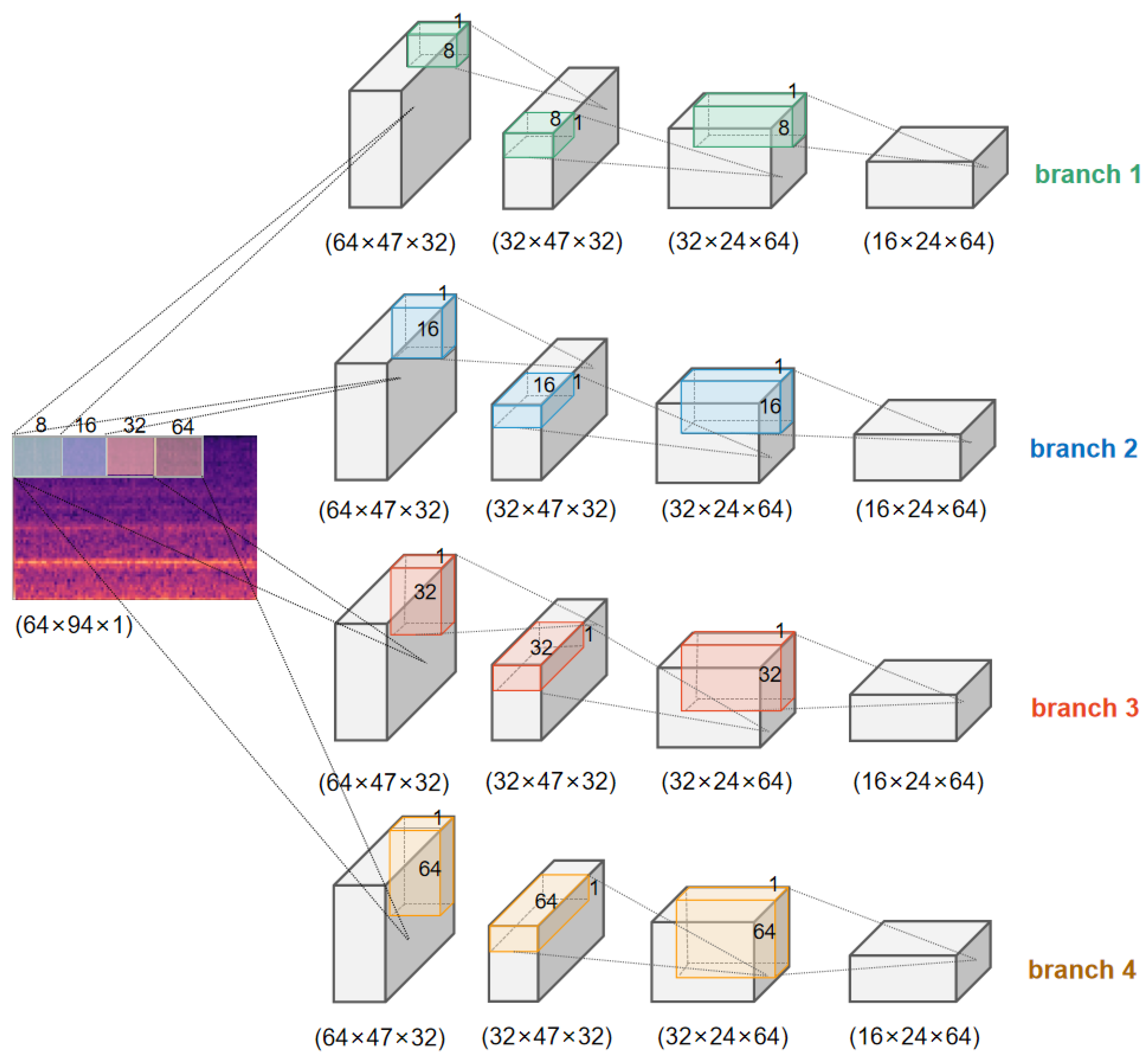
• The multi-scale convolutional learning structure extracts multi-scale features from Mel spectrograms, improving accuracy and adaptability in various acoustic signal scenarios.
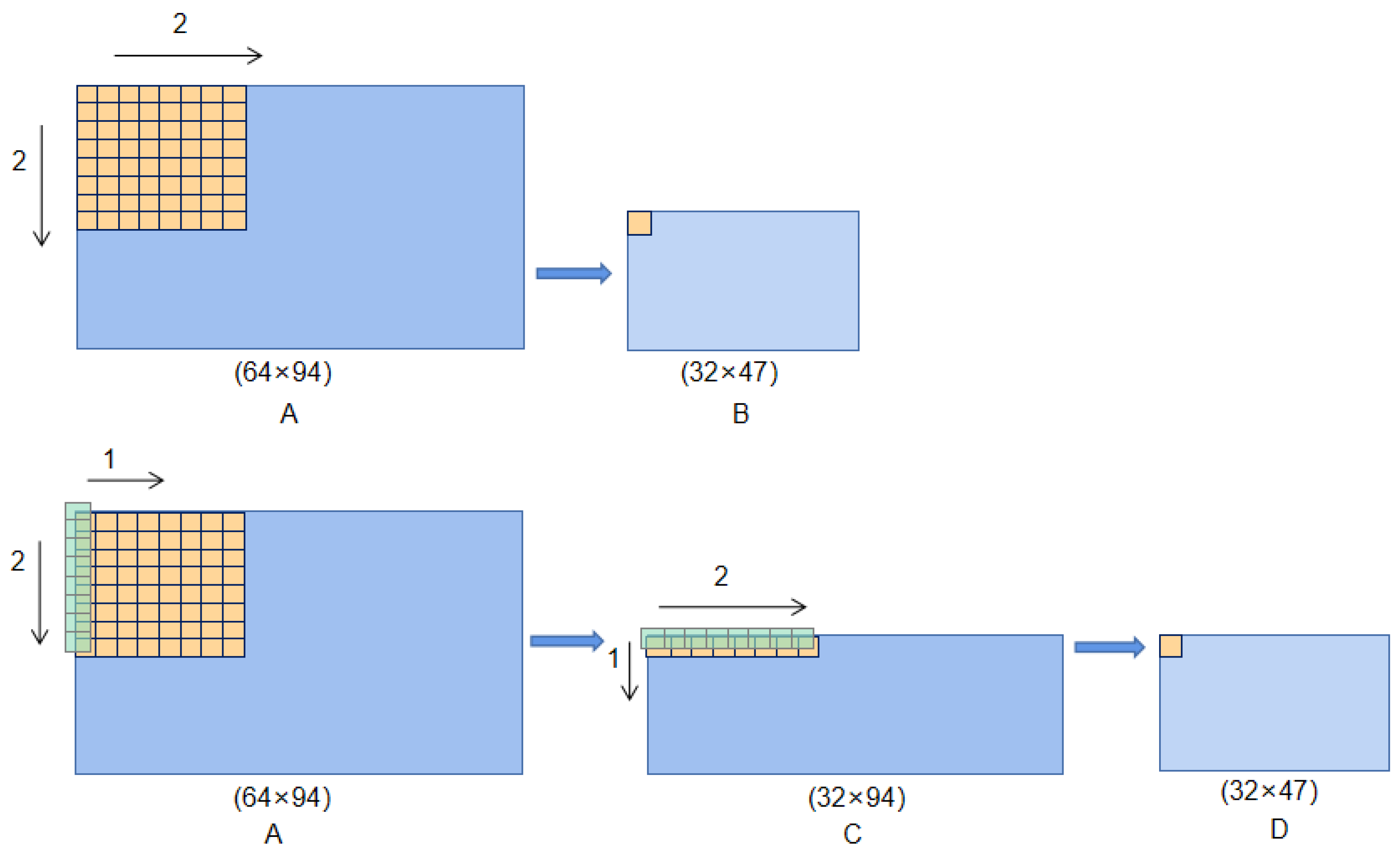
• The asymmetric convolution with horizontal and vertical kernels reduces parameters. Meanwhile, the asymmetric convolution can extract more stable low-frequency line spectrum features, which is beneficial for revealing the deep features of ship attributes.
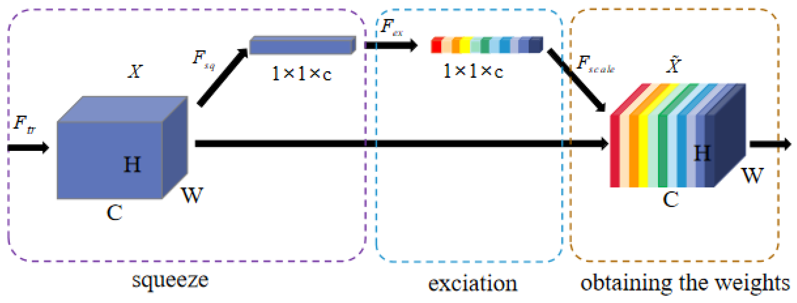
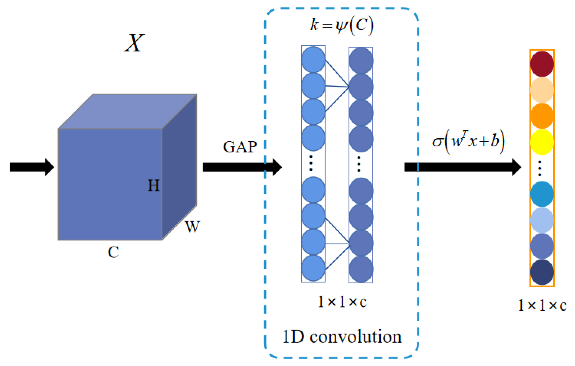
• The improved ECA attention mechanism fuses multi-scale features and emphasizes crucial features. To our knowledge, it is the first time that an ECA attention block has been introduced into the underwater acoustic target recognition field.

The paper is organized as follows: Section 2 elaborates on the flow of our method, namely feature preparing and MA-CNN-A structure. Section 3 introduces the DeepShip datasets. The experimental results and analysis are detailed in Section 4, and conclusions are presented in Section 5.

2. Materials and Methods

We provide an overview of our system. Then, we analyze the two primary components of the proposed method, i.e., the multi-scale asymmetric feature extraction and attention mechanism module.

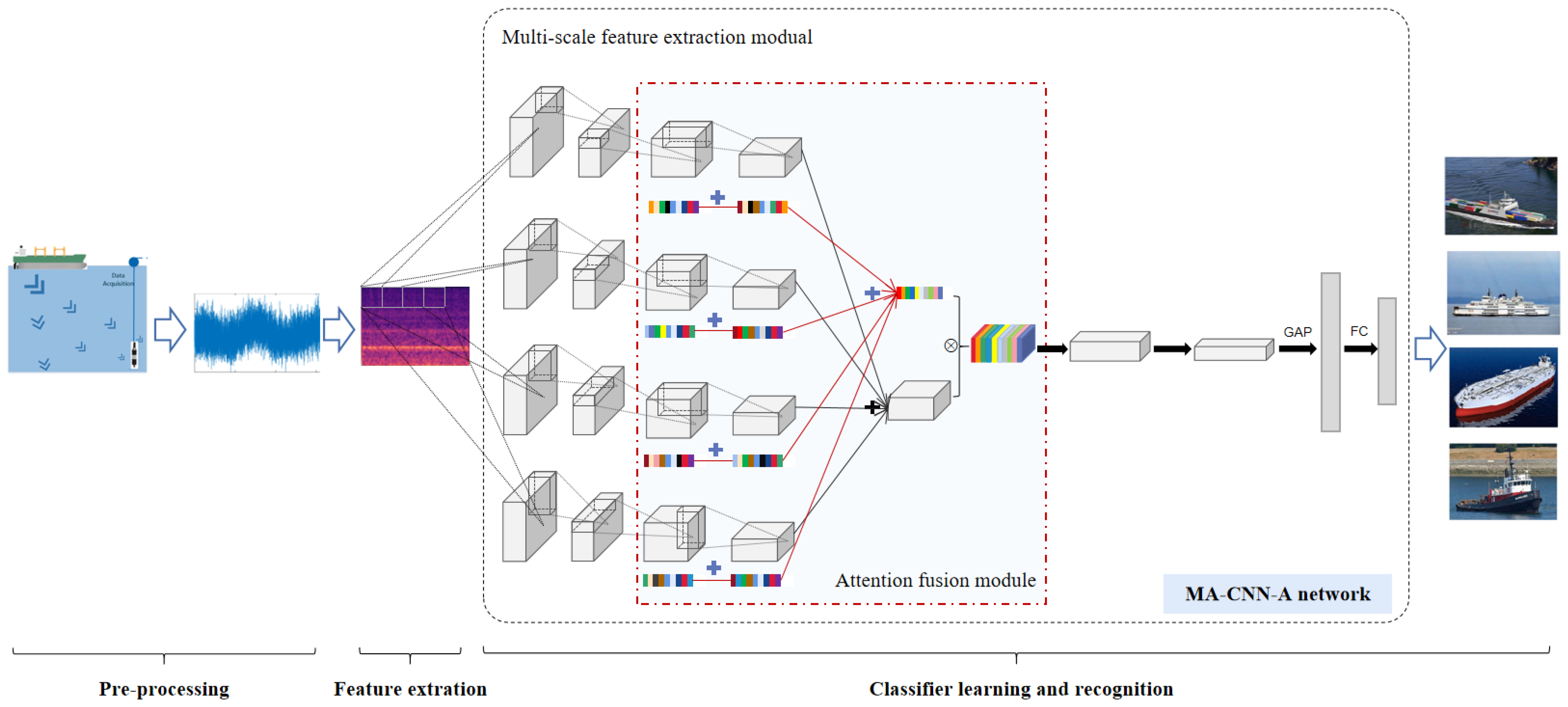
2.1. System Overview

Figure 1 offers a concise depiction of the proposed method in this paper. The process of our system could be divided into the three following stages:

• Data pre-processing. The sonar array initially captures ship-radiated noise. In this phase, array signal processing techniques (such as beamforming) strengthen the signals in target directions while reducing interference and noise from other sources.
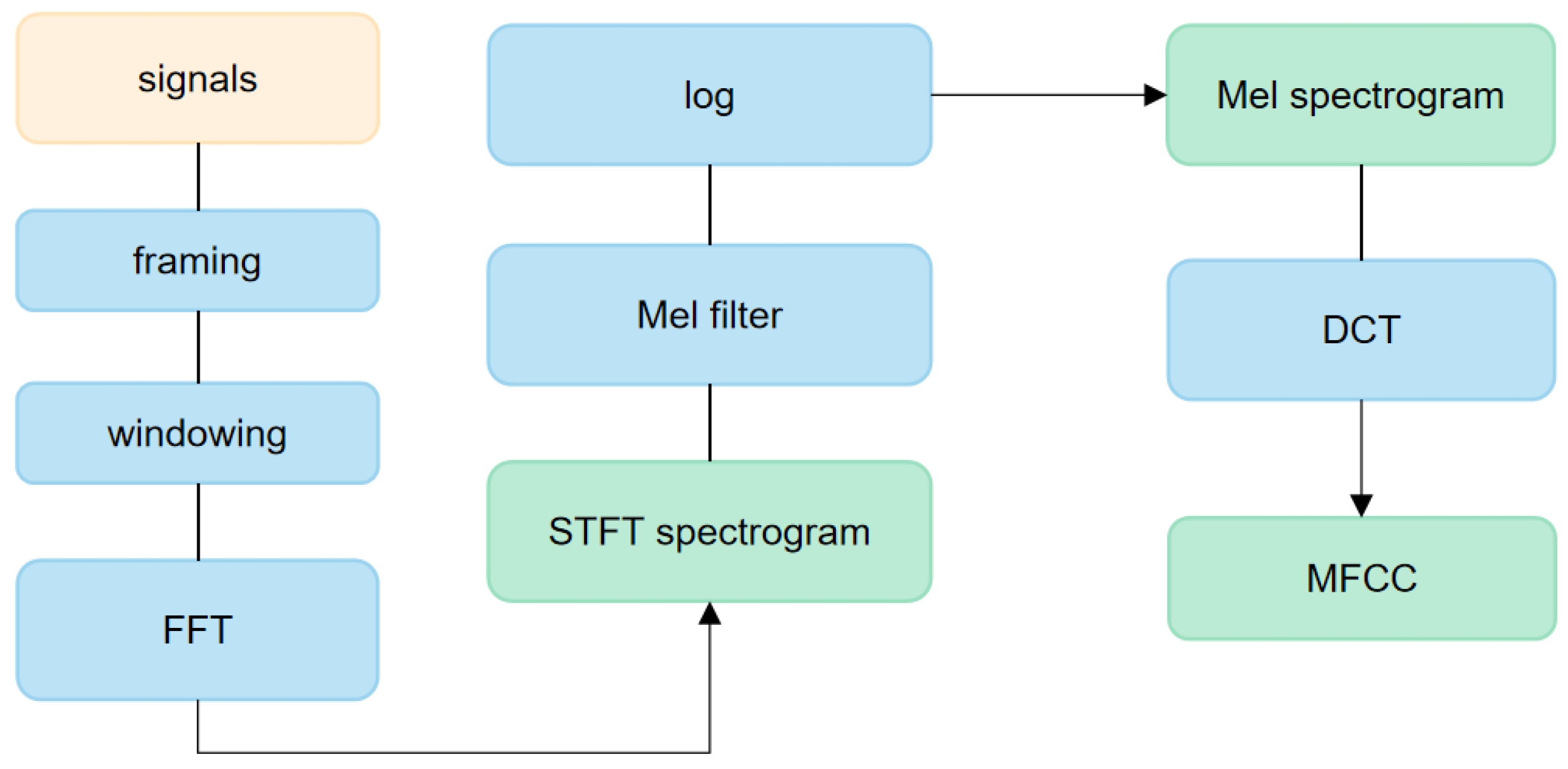
• Feature extraction. The audio signals are subsequently framed and converted into two-dimensional Mel spectrograms using Mel filters.
• Classifier learning and recognition. The Mel spectrograms are fed into the MA-CNN-A model. The MA-CNN-A will extract the detailed features and fuse the dominant feature weights by multi-scale asymmetric convolution and attention mechanisms. Finally, the fully connected layer with softmax is used as the classifier layer to obtain the predicted category label.

2.2. Feature Preparing

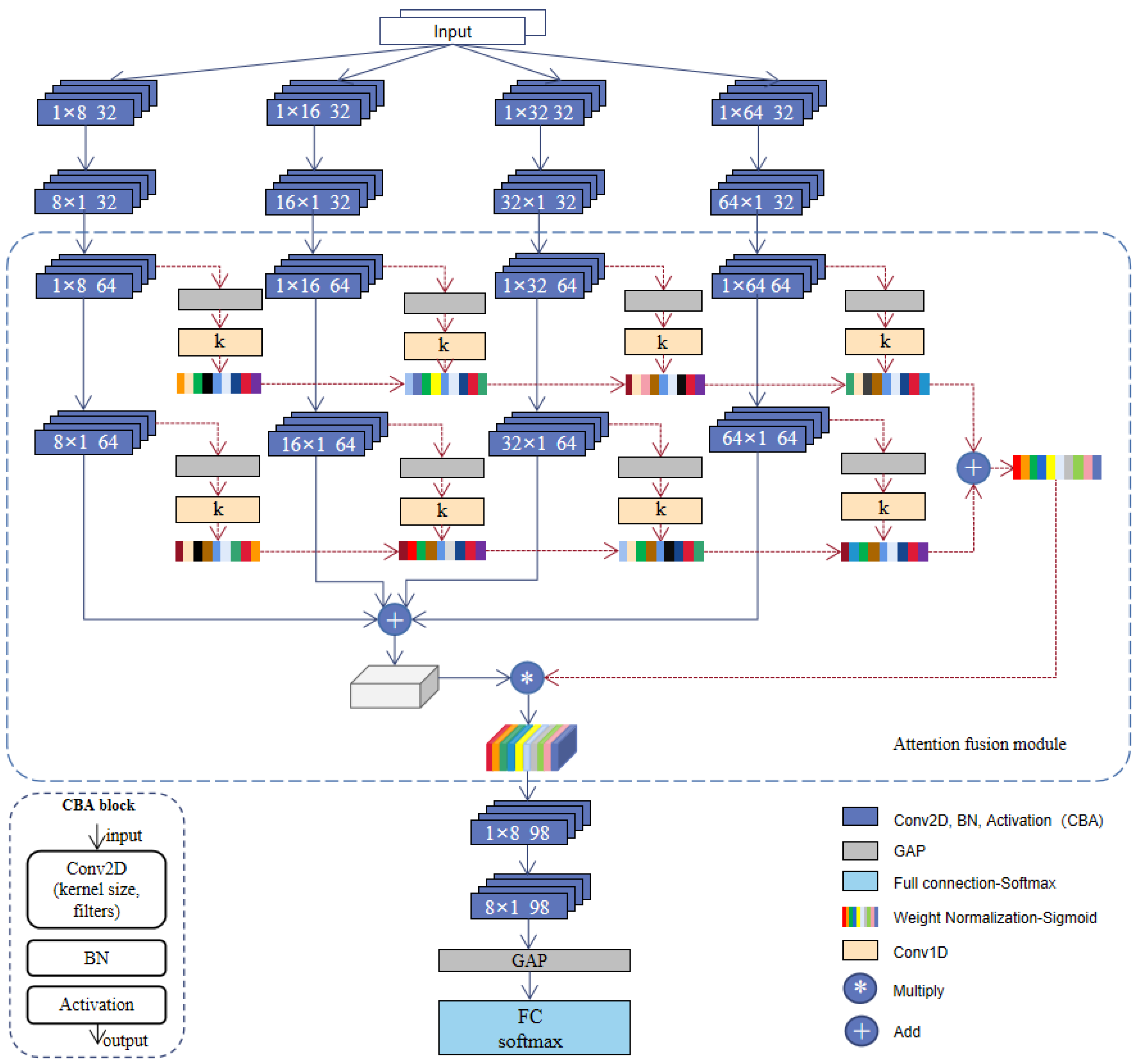
STFT contains a certain amount of redundant information for underwater acoustic target recognition, and its dimensions are relatively large, which brings greater computational complexity [24]. Inspired by the human hearing perception, the MFCC has emerged as a widely accepted method in acoustic signal processing. However, the discrete cosine transform (DCT) in the MFCC approach may filter out a substantial amount of valuable data [39]. Deep learning has a powerful ability to extract features, and researchers prefer to extract features from the Mel spectrogram which contains more information. The Mel-filter bank also performs better than other time–frequency methods in underwater acoustic target recognition [40]. Based on the aforementioned information, we choose the Mel spectrogram as the input of our network.

The process of Mel spectrogram extraction is shown in Figure 2. Initially, the complex FFT spectra are calculated through framing, windowing, and the application of the STFT. The magnitude of the STFT is integrated to produce the STFT spectrogram. Subsequently, Mel filter banks are applied to the spectrogram for filtering. Finally, the filtered spectra are transformed into Mel spectrograms by employing a logarithmic scale and an integration operation.

Figure 3 depicts the Mel spectrograms of four types of ship-radiated noises in the DeepShip dataset, i.e., cargo, passenger ship, oil tanker, and tug. The Mel spectrograms provide detailed visualizations in both the time and frequency domains. As depicted in Figure 3, there are noticeable differences in the energy concentration of the target-radiated noise in the low-frequency region. Specifically, the radiated noise from the cargo, oil tanker, and tug exhibits low energy levels above 500 Hz. The cargo ship has notable energy concentrations around 440 Hz, 220 Hz, and below 50 Hz. The tug’s energy mainly focuses around 450 Hz. The oil tanker displays robust energy distribution from 22 Hz to 130 Hz. The energy of the passenger ship concentrates around 920 Hz, with weaker energy distributions at other frequencies. Macroscopically, the distinct energy distributions for the four ship-radiated noises can serve as a foundation for classification. However, the inter-class differences in the Mel spectrograms of these ship noises are also significant, making traditional classification challenging and necessitating more discriminative feature extraction through deep learning.

2.3. MA-CNN-A Model

2.3.1. Multi-Scale Asymmetric Diverse Feature Extraction Backbone

As highlighted in Ref. [41], the square kernel convolution commonly used in CNN inadvertently reduces the training efficiency. In contrast, asymmetric convolution serves as a method to reduce the model parameters by approximating a larger square kernel convolutional layer using smaller kernels. This serves to factorize a standard two-dimensional convolution kernel into two one-dimension convolution kernels. That is to say, a $k\times 1$ convolution followed by a $1\times k$ convolution can substitute for a $k\times k$ convolution [33,41,42]. The mechanism can be expressed as:

$$I\times K^{\left(1\right)}+I\times K^{\left(2\right)}=I\times \left(K^{\left(1\right)}\oplus K^{\left(2\right)}\right)$$

(1)

where I is a matrix, $K^{\left(1\right)}$ and $K^{\left(2\right)}$ are two 2D kernels with compatible sizes, and ⊕ is the element-wise addition of the kernel parameters on the corresponding positions.

As depicted in Figure 4, a convolution operation with an $8\times 1$ kernel and a step size of $2\times 2$ is replaced by two sequential operations: first, an $8\times 1$ convolution kernel with a step size of $2\times 1$, and then a $1\times 8$ convolution kernel with a step size of $1\times 8$. In the following setup:

• Each $1\times 1$ region of feature map B perceives each $8\times 8$ region of feature map A.
• Each $1\times 8$ region of feature map C perceives every $8\times 8$ region of feature map A.
• Each $1\times 1$ region of feature map D perceives every $1\times 8$ region of feature map C.

Therefore, each $1\times 1$ region of feature map D is equivalent to each $8\times 8$ region of feature map A.

The Mel spectrogram has a unique physical meaning. One dimension of the Mel spectrogram represents time, and the other represents the frequency features of the time window. Since the two dimensions convey different information, extracting information processing across distinct dimensions can enhance the utilization of the information. For underwater acoustic target recognition, the main purpose of the asymmetric convolutional module is to allow the model to focus on important information in the time and frequency domains. Asymmetric convolution can enhance the model’s capacity to emphasize critical information within both the time and frequency domains. Inspired by the asymmetric convolutional module, we utilize two orthogonal asymmetric convolutions (horizontally and vertically) to capture features instead of a square convolution. In this way, it is not only possible to focus on essential information within the time and frequency domains, thereby mitigating background noise and eliminating the interference of redundant information, but also reduce the feature map size and the number of network parameters, thereby helping to alleviate network overfitting to some extent.

Furthermore, ship-radiated noise mainly consists of propeller, mechanical, and cavitation noise, primarily as low-frequency line spectra. Therefore, extracting low-frequency line spectrum features that remain stable over time is highly beneficial for identification. However, using square convolutions and sharing weights across frequency and time dimensions on the Mel spectrograms of ship-radiated noise may impair extracting physically meaningful features. When the convolution kernel shifts in the frequency dimension and the parameters are shared, it disrupts meaningful frequency positions. It has difficulty relating the extracted features to their original frequency points. Considering Mel spectrograms as the regular distribution of ship-radiated noise frequency components on the time axis, the vertical convolution kernel moves horizontally to process the features of the same time frame. This adjustment allows the kernel to extract frequency distribution features with translational invariance on the time axis, obtaining more stable line spectrum features. The movement of the horizontal convolution kernel works in the frequency domain to process the features of consecutive time frames, emphasizing the extraction of diverse features in the frequency domain obtaining more stable time features. Horizontal and vertical convolution are performed alternately, even if the time domain features are extracted first, and then the frequency domain features will be extracted based on this. A two-dimensional convolution is replaced by a set of horizontal or vertical convolutions, so focus on time domain extraction or frequency domain first, and the final results are similar. Based on the above analysis, we use asymmetric blocks to extract local key features cost-effectively. Moreover, this approach enables the extraction of more temporally stable low-frequency line spectrum features, which is beneficial for revealing deep features related to ship class attributes.

Traditional CNNs typically process images through a convolutional layer with a fixed filter size and stride to provide invariance to phase shifts and down-sample the signals. Ship-radiated noise contains a broad frequency range. Smaller filters emphasize the overall structure, while larger filters reveal specific details in spectrograms. As a result, relying on a fixed filter size for feature extraction may not leverage the full potential of Mel spectrograms, limiting the ability to build a discriminative representation for diverse patterns.

Considering the above, we proposed a multi-scale convolutional method to capture the diverse features from the Mel spectrogram. As depicted in Figure 5, our proposed network utilizes a multi-scale extraction backbone with asymmetric blocks. It is structured with four branches, each employing convolution kernels of distinct sizes, i.e., 8, 16, 32, and 64. These kernels ensure the extraction of multi-scale difference features and each branch further integrates asymmetric blocks. That is to say, in order to obtain features from the different receptive fields, we use multiple branches to extract different features. However, too many branches will increase the redundancy and complexity of the model. After weighing both the model complexity and accuracy, we settle on four branches in the backbone.

2.3.2. Attention Mechanism-Based Multi-Scale Feature Fusion

In order to further eliminate the aforementioned redundancy, we introduce the channel weighting mechanism into the proposed network. It reasonably allocates weights to the information in different channels and effectively removes channels with similar characteristics. A notable example of a channel attention mechanism is the SE module [26], which has enhanced several deep CNN architectures.

In Figure 6, the SE block begins with GAP, obtaining the data with dimensions of $1\times 1\times C$. Subsequently, two fully connected layers are utilized to determine the channel weights. The first fully connected layer compresses the number of channels to C to reduce the parameter size and employs the ReLU activation function. Subsequently, the second fully connected layer restores the channels to C and employs the Sigmoid activation function, generating weight values within the $\left[0,1\right]$ range. Finally, these weight values are multiplied by X to obtain $\tilde{X}$. Although the SE module is widely used in CNNs, previous studies have shown that the dimension reduction in SE block brings a side effect. Such a dimension reduction may harm learning the dependencies between the channels for underwater signals.

Some researchers improved the SE block by combining it with additional spatial attention or capturing more sophisticated channel-wise dependencies [43,44]. Although these methods achieved higher accuracy, they often bring higher model complexity and suffer from a heavier computational burden. To solve the problem of dimension reduction and design channel attention in a more efficient way, Wang et al. [28] introduced the ECA module, which offers notable performance enhancements with just a few additional parameters. The ECA module employs a local cross-channel interaction approach, efficiently executed through 1D convolution without reducing dimensionality. Moreover, the ECA can adaptively determine the 1D convolution kernel size, thus defining the scope of local cross-channel interactions. We improved the ECA based on the characteristics of our backbone model and applied the improved ECA block to underwater acoustic target recognition. The part of the ECA module we adopted is depicted in Figure 7. Initially, the input feature layer undergoes GAP, transforming the data dimension to $1\times 1\times C$. Subsequently, the fully connected layer in the SE module is substituted with a 1D convolution operation, where k is proportionate to the channel dimension. Finally, the weight values are generated using the Sigmoid activation function.

As shown in Figure 8, we introduce the MA-CNN-A model. The backbone of MA-CNN-A is formed by four branches of feature extraction blocks (with scales of 8, 16, 32, and 64) and eight asymmetric convolution kernel shapes (namely $1\times 8$, $8\times 1$, $1\times 16$, $16\times 1$, $1\times 32$, $32\times 1$, $1\times 64$, and $64\times 1$) to decrease the parameters and capture deep features related to ship-radiated noise class attributes. Subsequently, we add features from the four branches instead of concatenating, which increases the amount of feature information and decreases the cost of the model’s memory compared with concatenation. Simultaneously, our attention mechanism improves the ECA module based on our backbone. We can obtain the weight value from eight distinct convolution blocks to enrich the array of channel weight values. The weight values are added together rather than multiplied by the original convolution layer, obtaining a comprehensive weight value. The comprehensive weight value is multiplied by the features added from four channels to rebalance the feature weights. After that, the architecture is further strengthened with additional asymmetric convolutions and GAP layers. The ReLU nonlinear activation function is adopted by each convolutional operation except for the fully connected layer. Finally, a fully connected layer with softmax is used as a classifier.

3. Experiment Setup

3.1. Dataset

We conducted experiments using a publicly available dataset called DeepShip [13]. DeepShip is a recent benchmark for underwater acoustics. It contains 47 h and 4 min of real-world underwater recordings from 265 ships. The ships are labeled into four types, i.e., cargo, passenger ship, tanker, and tug. The actual dataset used in our study was a subset of the entire recording.

We resampled the data with a frequency of 16 kHz. To jointly consider the feature size, accuracy, and computational resources, we segmented all audio files into three-second segments and obtained 20,000 samples. Specifically, using segments of inappropriate lengths may lead to issues. Long segments often provide more excellent stability and enhance the classification outcomes due to the impact of burst noise. While using excessively long segments increases the computational complexity and demands more computing resources [45]. Subsequently, the 20,000 samples are distributed in a ratio of 7:2:1, resulting in 14,000, 4000, and 2000 segments for the training, validation, and test sets, respectively. Detailed information about DeepShip dataset and partitions are listed in

Table 1. DeespShip benchmark dataset summary and partitions.

Ship Type	No. of Ships	Total Recordings	Training Size	Validation Size	Test Size
Cargo	69	110	3500	1000	500
Passenger ship	46	193	3500	1000	500
Oil tanker	133	240	3500	1000	500
Tug	17	70	3500	1000	500

.

3.2. Parameters Setup

Each three-second segment is windowed into short frames of 1024 and hopped by 512. It results in 94 frames for each segment signal based on the specified frame and hop sizes. From the 94 frames, the Mel spectrogram of the segment is computed. Finally, each segment is saved as a Mel spectrogram, with dimensions specified in

Table 2. The generation parameters of Mel spectrograms (Melsp).

Feature	Dimension	Sampling Rate	N-fft	Hop Length
Melsp	64 × 94	16 kHz	1024	512

.

All experiments are conducted using TensorFlow 2.6.2 with Python version 3.6 and verified by a computer with a GPU of NVIDIA Geforce RTX 2080Ti and Core(TM)i7-7820X [email protected] GHZ (EVGA Corporation, Brea, CA, USA). The cross-entropy loss J is used as the loss function, which is shown as follows:

$$J=-\sum _{i=0}^N{y}_{i}lg\left({\widehat{y}}_i\right)$$

(2)

where $y_i$ and ${\widehat{y}}_i$ are the actual and predictive outputs of the softmax classifier, respectively. N represents the number of categories.

The hyperparameters of the network model are determined by repeated experiments. Specifically, the initial learning rate was set to $1\times {10}^{-2}$. We initialized the model parameters following a Gaussian distribution to mitigate potential challenges related to gradient vanishing and explosion. A batch size of 16 was adopted for training. We incorporated an early stopping mechanism to reduce overfitting, setting the patience value to 10.

3.3. Evaluation Metric

The performance of all algorithms used in this study is assessed using the following metrics, i.e., $Accuracy$, $Precision$, $Recall$, and $F1-Score$.

$Accuracy$ is calculated using the following expression:

$$Accuracy=\frac{TP+TN}{TP+TN+FP+FN}$$

(3)

where $TP$ is true positive, $TN$ is true negative, $FP$ is false positive, and $FN$ is false negative.

$Precision$ is computed as:

$$Precision=\frac{TP}{TP+FP}$$

(4)

$Recall$ is computed as:

$$Recall=\frac{TP}{TP+FN}$$

(5)

$F1-Score$ is computed as:

$$F1-Score=2\times \frac{precision\times recall}{precision+recall}$$

(6)

3.4. Comparative Methods

In our comparative experiments, we evaluated the efficacy of the MA-CNN-A in performance with other methods, including ResNet18 [46], EfficientNetv2 [47], and lightweight architectures like MobileNetv2 [32] and ShuffleNetv2 [48]. Moreover, our method was compared with two ship-radiated noise classification methods conducted on DeepShip, i.e., the Transformer [49] and convolutional recurrent neural networks (CRNNs) [24].

ResNet18: The central design of ResNet is the residual block. ResNet has demonstrated commendable performance in the underwater acoustic target recognition domain. We adopt the classical ResNet18 architecture as a comparative classification model.

EfficientNetv2: EfficientNetv2 has exhibited a robust performance in image recognition. It introduces a compound scaling method that efficiently scales the model across multiple dimensions to strike a better balance.

MobileNetv2: MobileNetv2 is a light-weight neural network model widely applied in time–frequency-based underwater acoustic target recognition. Its design is underscored by inverted residual modules and linear bottlenecks.

ShuffleNetv2: ShuffleNetv2 is also a lightweight neural network model. It combines the pointwise group convolution and channel concatenation to reduce the computational cost. ShuffleNetv2 has also been widely used in underwater acoustic target recognition [50].

Transformer: Transformer is one of the hottest models today. It can directly obtain global information about the features. Ref. [49] proposed a transformer model based on DeepShip, which will be compared with ours.

CRNN: The CRNN architecture presents significant merits when handling time-series signals. Its efficacy has been corroborated across diverse real-world datasets in speech recognition and environmental acoustic detection. Ref. [24] proposed a CRNN for ship-radiated noise classification.

4. Experiment Results and Analysis

The experiments are structured in three aspects. We analyzed the result of the proposed method and compared it with other methods. Then, ablation studies prove the efficiency of the multi-scale asymmetric convolution and the attention mechanism. Finally, we test the robustness of the MA-CNN-A model.

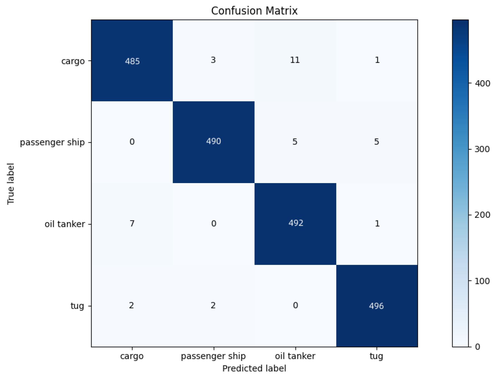
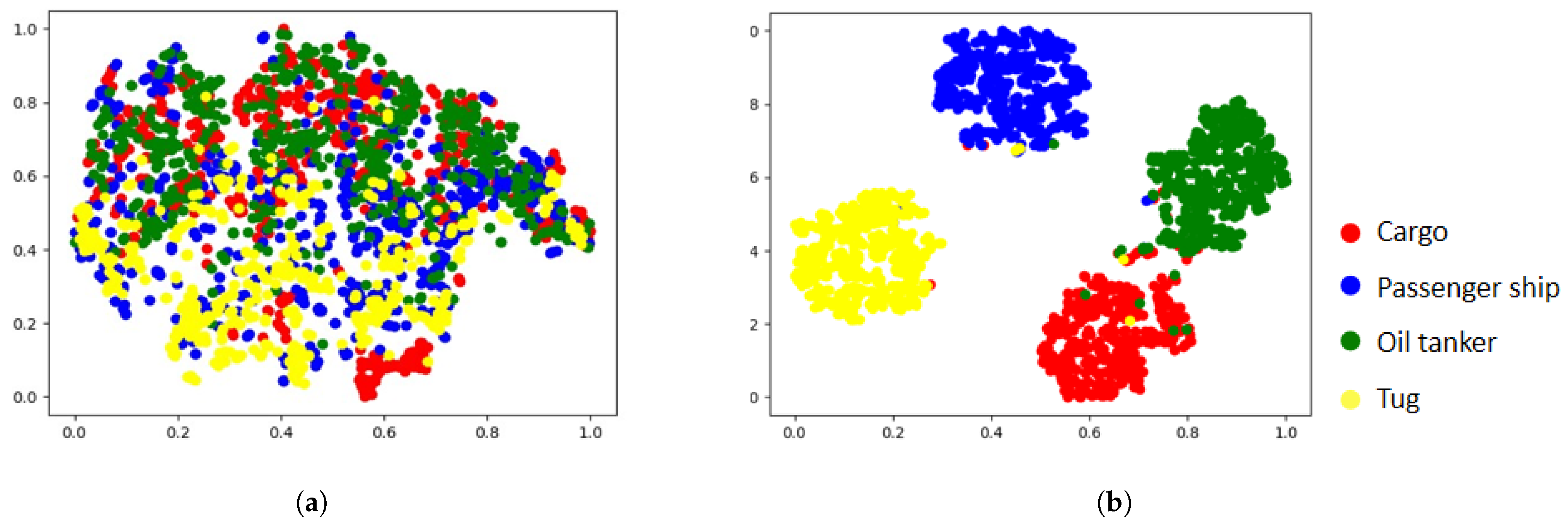
4.1. The Result of MA-CNN-A Model

Figure 9 shows the confusion matrix of the MA-CNN-A network. As depicted in Figure 9, the MA-CNN-A has excellent recognition performance for each type of ship. The tug ship exhibits the highest recognition accuracy, potentially attributable to its pronounced material and size disparities compared to the other three ship categories. There is a slight misclassification between cargo ships and tankers relative to other ships. One plausible explanation for this trend might be the nature of the training datasets corresponding to the cargo and oil tankers. Specifically, these datasets comprise more extensive and acoustically intricate audio files, thereby complicating the recognition.

Table 3. The results of MA-CNN-A on DeepShip dataset.

	$\mathit{Precision}$	$\mathit{Recall}$	$\mathit{F}1-\mathit{Score}$
Cargo	98.1%	97.0%	97.6%
Passenger ship	99.0%	98.0%	98.5%
Oil tanker	96.9%	98.4%	97.6%
Tug	98.6%	99.2%	98.9%
Overall average	98.2%

delineates the recognition results for the MA-CNN-A model. MA-CNN-A achieves an overall accuracy of 98.2%. The tug emerges with the highest recognition accuracy of 99.2%.

The t-distributed stochastic neighbor embedding (t-SNE) data visualization is a technique to visually analyze high-dimensional features. These features are represented in a two-dimensional space. Our visualization is constructed using the testing data, as depicted in Figure 10. The figure comprises four distinct types of ships, each differentiated by color, with each color signifying a type of ship. Figure 10a delineates the distance characteristics using the Mel spectrogram as the input, which indicates that the Mel spectrogram offers limited separability. From Figure 10b, it can be observed that the ships derived from the GAP layer of MA-CNN-A tend to cluster together, indicating that the multi-scale features extracted by MA-CNN-A have a favorable effect.

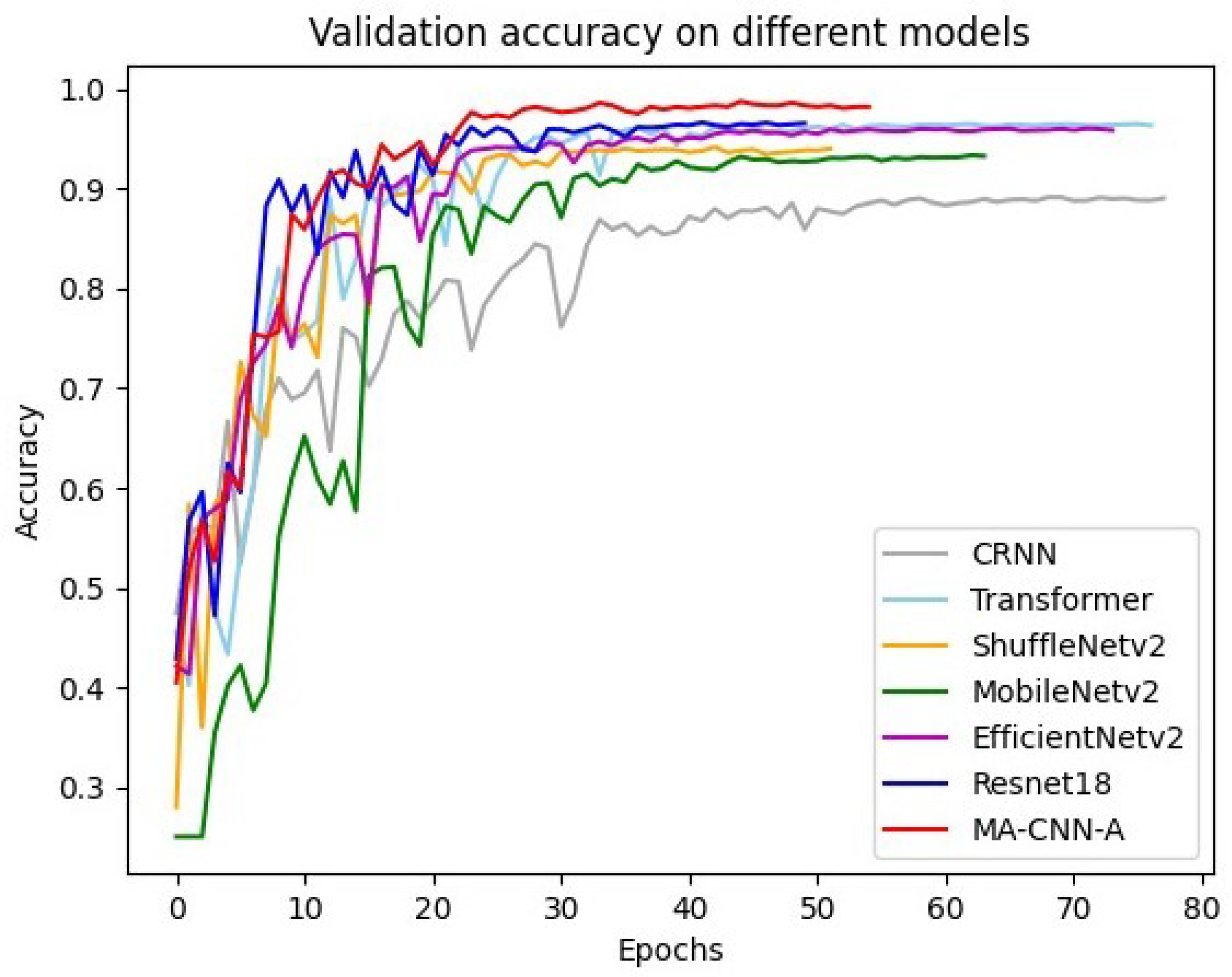
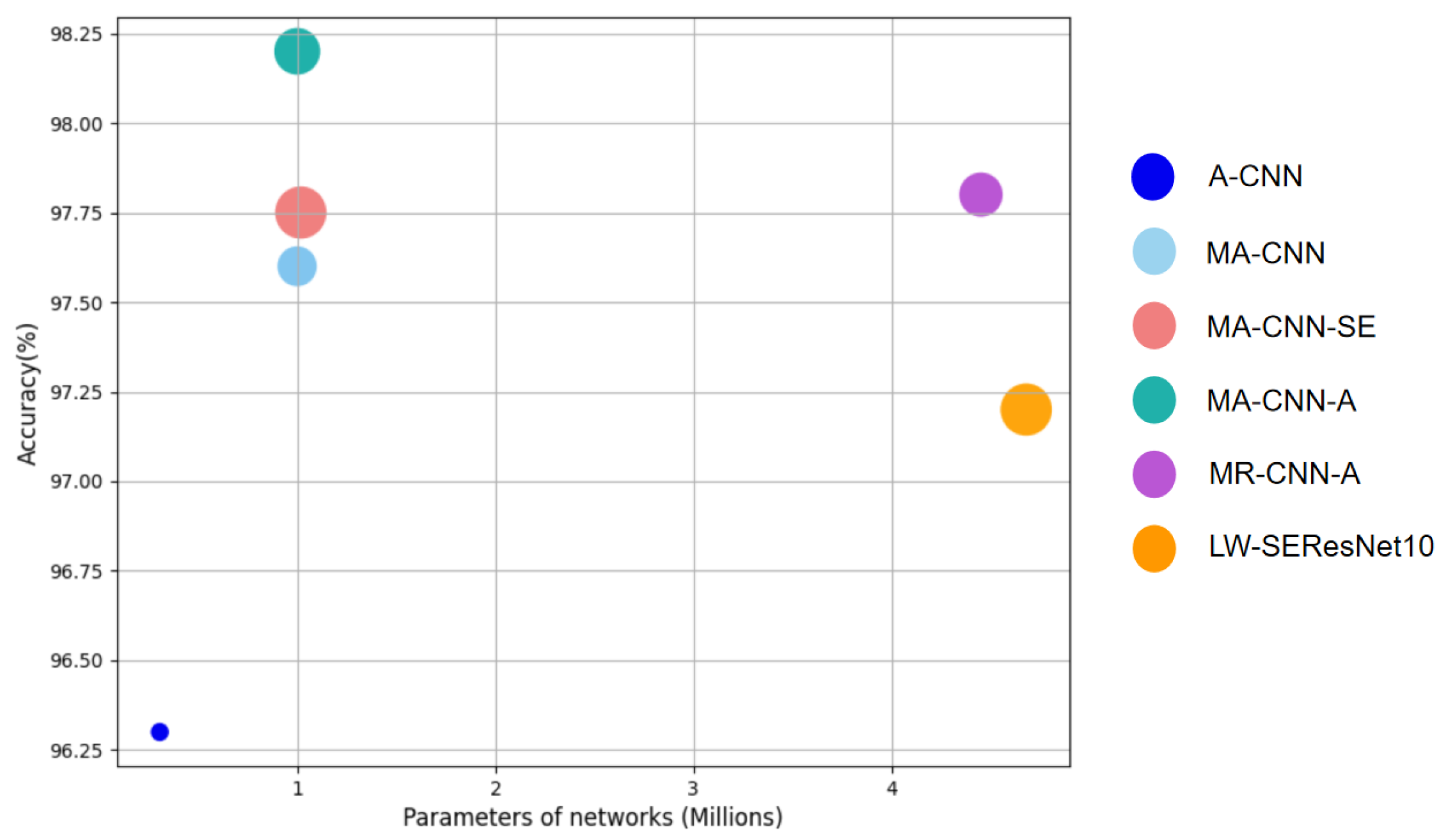
4.2. Comparison of Different Methods

The Mel spectrogram generator and no data augmentation employed in the MA-CNN-A are also used in the models from Section 3.4. Figure 11 displays the validation accuracy results for the seven models. It is evident that the MA-CNN-A demonstrates a rapid convergence rate and achieves the highest accuracy.

To comprehensively evaluate the prediction performances, we evaluated each model’s accuracy, the number of parameters (denoted as No. params), and inference speed, which is measured in frames per second (fps). Fps refers to how many frames of audio data the model can process each second in

Table 4. Comparative experimental results on the DeepShip dataset.

Model	Accuracy (%)	Computation Time (s/epoch)	Inference Speed on GPU (fps)	Inference Speed on CPU (fps)	GFLOPs	No. Params (M)	Model Size (MB)
MA-CNN-A	98.2%	28	310.2	123.5	1.177	1.00	3.9
ResNet18 [46]	96.3%	38	265.8	23.1	6.592	11.18	42.7
EfficientNetv2 [47]	96.3%	110	49.8	41.5	0.708	20.34	78.0
MobileNetv2 [32]	94.7%	36	267.7	86.9	0.073	2.26	12.3
ShuffleNetv2 [48]	95.1%	39	168.4	143.5	0.029	1.20	4.7
Transformer [49]	95.3%	35	230.8	101.1	4.134	2.55	9.0
CRNN [24]	88.4%	42	108.4	50.6	6.240	6.81	24.2

.

Regarding recognition accuracy, the MA-CNN-A distinctly stands out with a performance of 98.2%, highlighting its robustness and superior generalization capabilities. Regarding computational efficiency, it can be observed that the number of FLOPs of the proposed method MA-CNN-A is lower than ResNet18, Transformer, and CRNN. In the case of the computation time, the time taken by MA-CNN-A is less than that of all the models. The low FLOPs and computation time indicate that our model requires fewer computational resources, which is a distinct advantage in power-constrained underwater deployment scenarios. Additionally, MA-CNN-A achieves the fastest inference speed of 310.2 fps on GPU and offers an inference speed of 123.5 fps on CPU. Regarding the model complexity, the number of parameters of MA-CNN-A is just 1.00 M, and the model size of MA-CNN-A is just 3.9 MB, which is significantly smaller than the other models. The compactness makes deploying and running on underwater devices with limited memory more feasible.

In summary, the comparison results demonstrate that the MA-CNN-A network possesses a significantly higher recognition accuracy while maintaining relatively fewer model parameters and a faster inference speed, outperforming other representative models.

4.3. Ablation Experiments

To further provide information on our method, we conducted ablation experiments to validate the effectiveness of the multi-scale asymmetric and our attention mechanism. First, we demonstrated the effectiveness of the multi-scale asymmetric convolution.

Table 5. Comparison of the recognition results for asymmetric convolutions and square convolutions with different channels.

No. of Branches	Kernal Shape	Kernal Size	Stride	Accuracy	No. of Parameters (M)
One	Square	(8 × 8)	(2 × 2)	95.5%	0.54
	Asymmetric	(1 × 8) (8 × 1)	(1 × 2) (2 × 1)	96.3%	0.19
Two	Square	(8 × 8) (16 × 16)	(2 × 2)	96.6%	1.07
	Asymmetric	(1 × 8) (8 × 1)	(1 × 2) (2 × 1)	97.0%	0.30
		(1 × 16) (16 × 1)
Three	Square	(8 × 8) (16 × 16)	(2 × 2)	97.3%	3.12
		(32 × 32)
	Asymmetric	(1 × 8) (8 × 1)	(1 × 2) (2 × 1)	97.4%	0.53
		(1 × 16) (16 × 1)
		(1 × 32) (32 × 1)
Four	Square	(8 × 8) (16 × 16)	(2 × 2)	96.3%	11.72
		(32 × 32) (64 × 64)
	Asymmetric	(1 × 8) (8 × 1)	(1 × 2) (2 × 1)	97.6%	1.00
		(1 × 16) (16 × 1)
		(1 × 32) (32 × 1)
		(1 × 64) (64 × 1)
Five	Square	(8 × 8) (16 × 16)	(2 × 2)	97.3%	45.80
		(32 × 32) (64 × 64)
		(128 × 128)
	Asymmetric	(1 × 8) (8 × 1)	(1 × 2) (2 × 1)	97.6%	1.92
		(1 × 16) (16 × 1)
		(1 × 32) (32 × 1)
		(1 × 64) (64 × 1)
		(1 × 128) (128 × 1)

presents recognition results from asymmetric and square convolutions with different scales. It should be noted that the experiments presented in Table 5 do not introduce any attention mechanism.

Comparing the effect of multi-scale to fixed-scale convolutions, it is evident that multi-scale difference feature extraction consistently outperforms the fixed-scale, irrespective of whether the convolution is square or asymmetric. Specifically, the accuracy achieves 97.3% by three branches of square convolutions, obtaining an improvement of 1.8% compared to the fixed-scale square convolution. When implemented with four branches, the asymmetric convolution obtained the highest recognition accuracy of 97.6%, which improves to 1.8% over fixed-scale asymmetric convolutions. Subsequently, even if other scale feature extraction branches are added, redundant features may be extracted, which has little impact on the classification accuracy. Our experiments validate the decision to employ the four branches of the asymmetric block as the backbone for differential feature extraction. Regarding the performance of asymmetric convolution, asymmetric convolutions achieve superior accuracy and possess fewer parameters than square convolution kernels. Comparing the parameters of four branches of asymmetric CNNs and three branches of square CNNs, the former have a 68.1% reduction in parameters.

Regarding the performance of our attention mechanism, Figure 12 compares multi-scale asymmetric convolution (MA-CNN) and the introduction of various attention mechanisms with respect to the accuracy, number of model parameters, and floating point operations (FLOPs). The compared attention mechanisms are as follows: the multi-scale asymmetric CNN based on the SE attention mechanism (MA-CNN-SE); the MA-CNN-A, a lightweight squeeze and excitation residual network [50] (LW-SEResNet10); and multi-scale residual convolutional neural network [51] (MR-CNN-A), embedded with an SE attention mechanism. As shown in Figure 12, the MA-CNN model reaches an accuracy of 97.6% and makes an improvement of 1.3% over A-CNN and LW-SEResNet10. It shows that multi-scale feature extraction is effective. Compared with MA-CNN, our attention mechanism introduces very few additional parameters and negligible computations while bringing notable performance gain. Specifically, for MA-CNN with 0.996 M parameters and 1.18 GFLOPs, the additional parameters and computations of MA-CNN-A are 24 and 3.23 × 10${}^{-4}$ GFLOPs, respectively. Furthermore, the accuracy of MA-CNN-A makes improvements of 0.6%, 0.5%, 1.0%, and 0.4% over the MA-CNN, MA-CNN-SE, LW-SEResNet10, and MR-CNN-A, respectively.

4.4. Robustness Test

We add white Gaussian noise to the test data at different SNRs. Additionally, we assess the adaptability of MA-CNN-A by inputting different features.

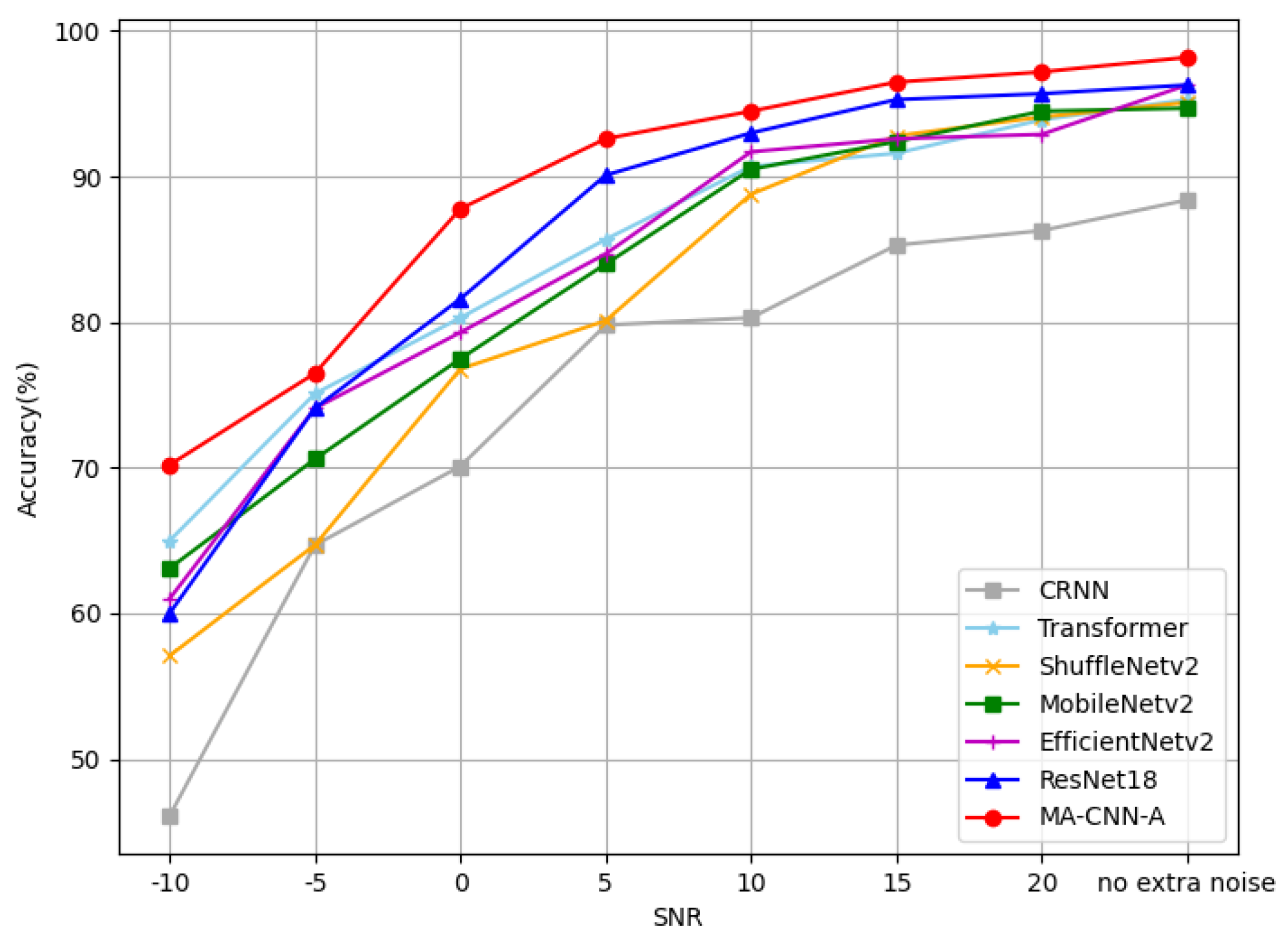
4.4.1. Test on Low SNR

In this experiment, the original dataset signals already contain environmental noise. Due to data collection constraints, such as real-time signal variation, it is challenging to define a noise standard under the constraints. Therefore, this study denotes the power of the dataset signals as $P_s$. The power of added Gaussian noises is denoted by $P_n$. The SNR is defined as follows:

$$SNR=10log\left(\frac{P_s}{P_n}\right)$$

(7)

As illustrated in Figure 13, seven methods are assessed on the DeepShip dataset across various SNRs. Within the SNR range of −10–20 dB, the accuracy of the MA-CNN-A network consistently outperforms the other networks, demonstrating its robust recognition capabilities for underwater acoustic signals with different SNRs. Specifically, within the SNR range of 5 dB to 20 dB, ResNet18 ranks second in performance. This may be attributed to the network easily causing gradient vanishing during backpropagation under high SNR, while ResNet18 effectively avoids gradient vanishing. However, when the SNR decreases from 5 dB to −10 dB, the accuracy of the ResNet18 significantly declines. It may be attributed to the original waveform of the signal getting submerged in the noise. Therefore, the corresponding Mel spectrogram contains much noise and a small amount of feature information. Many extracted features are noise-related and do not contribute to accuracy. In contrast, the accuracy of MA-CNN-A degrades relatively slowly. When the SNR is 10, MA-CNN-A has 1.5%, 2.8%, 4.0%, 5.7%, 3.8%, and 14.2% performance advantages on ResNet18, EfficientNetv2, MobileNetv2, ShuffleNetv2, Transformer, and CRNN, respectively. When the noise gradually increases until the SNR is 0, the gap widens to 6.2%, 8.5%, 10.3%, 11.0%, 7.5%, and 17.7%.

The aforementioned results show the significance of multi-scale asymmetric convolution in extracting features at varying resolutions. Moreover, our attention mechanism can eliminate the feature channels that do not contribute to the recognition effect. Thus, in challenging low-SNR scenarios, the MA-CNN-A distinctly excels compared with other models.

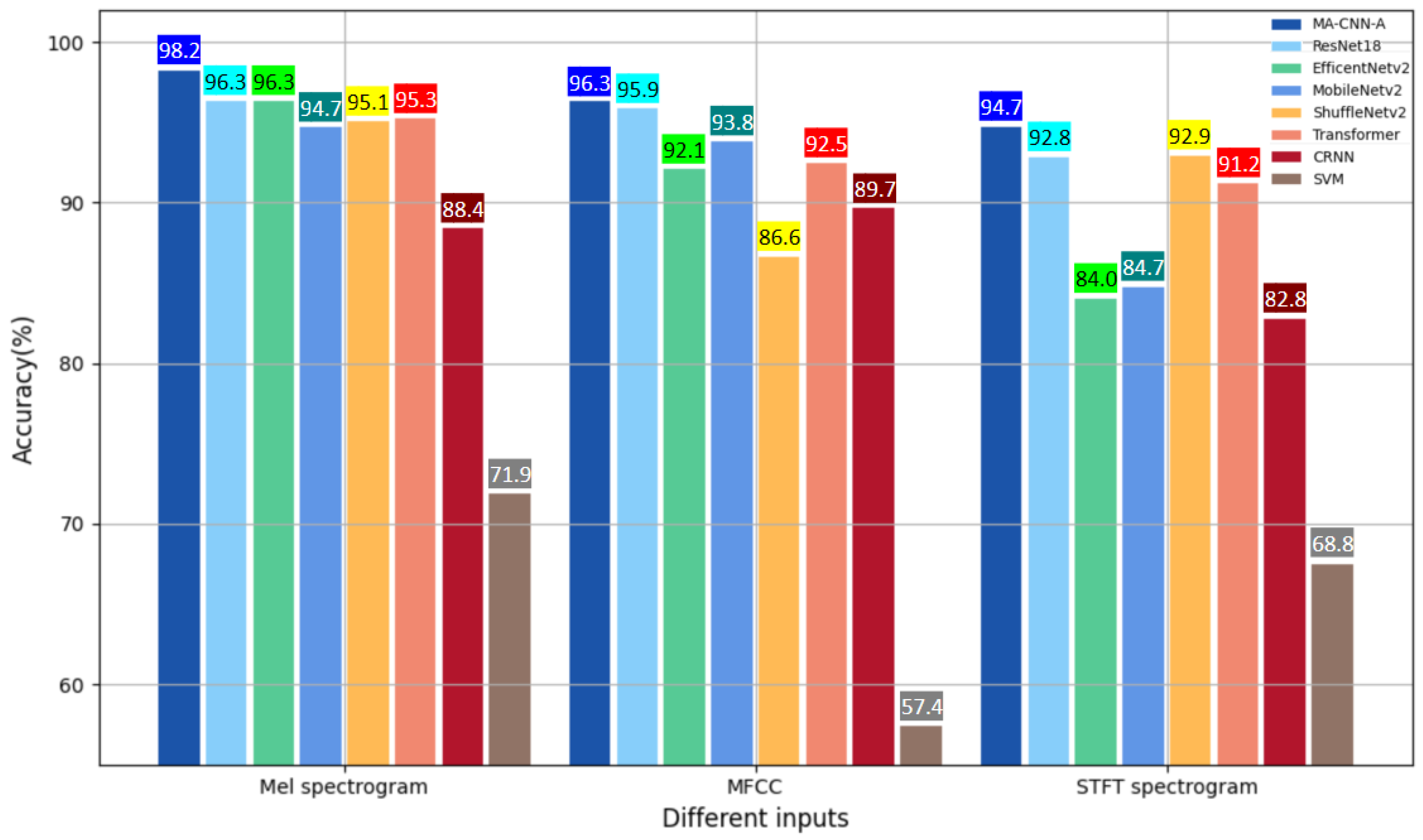
4.4.2. Performance of Different Features

To validate the adaptability of the network to other inputs, we examined its recognition capabilities using different features, such as the STFT spectrogram and MFCC. Figure 14 shows that traditional machine learning methods such as SVM cannot classify ship radiation noise well. MA-CNN-A significantly outperforms other networks under different features. Specifically, the accuracy of MA-CNN-A stands at 98.2%, 96.3%, and 94.7% on the Mel spectrogram, MFCC, and STFT spectrogram, respectively. The results suggest that our model consistently maintains a relatively good recognition performance for different inputs. Additionally, the accuracy of ResNet18 is close to MA-CNN-A. However, the ResNet18 has a relatively larger model and does not do well in experiments against noise. Therefore, MA-CNN-A outperforms in identifying features from diverse time–frequency representations of ship-radiated noise signals.

5. Conclusions

This paper introduces a lightweight network model named MA-CNN-A for ship-radiated noise classification. The model adopts multi-scale convolutions for more detailed feature extraction. The improved ECA attention mechanism also rebalances the weight across feature channels and integrates multi-scale features. We use the asymmetric convolution with horizontal and vertical kernels to reduce the parameter size. Moreover, the asymmetric convolution can extract more stable low-frequency line spectrum features, which is beneficial for revealing the deep features of ship attributes. Compared with several lightweight CNNs, the MA-CNN-A significantly reduces parameters and improves recognition accuracy.

Experiments on the DeepShip dataset show that MA-CNN-A achieves an accuracy of 98.2%, outperforming several other mainstream deep learning models. Ablation explorations confirm the benefits of the multi-scale asymmetric convolutions and the attention mechanism. It is worth noting that MA-CNN-A maintains robust stability in Gaussian noise and exhibits significant adaptability to different inputs.

References

1. Ke, X.; Yuan, F.; Cheng, E. Integrated optimization of underwater acoustic ship-radiated noise recognition based on two-dimensional feature fusion. Appl. Acoust. 2020, 159, 107057. [Google Scholar] [CrossRef]
2. Li, Y.; Li, Y.; Chen, X.; Yu, J. Denoising and feature extraction algorithms using NPE combined with VMD and their applications in ship-radiated noise. Symmetry 2017, 9, 256. [Google Scholar] [CrossRef]
3. Li, J.; Yang, H. The underwater acoustic target timbre perception and recognition based on the auditory inspired deep convolutional neural network. Appl. Acoust. 2021, 182, 108210. [Google Scholar] [CrossRef]
4. Das, A.; Kumar, A.; Bahl, R. Marine vessel classification based on passive sonar data: The cepstrum-based approach. IET Radar Sonar Nav. 2013, 7, 87–93. [Google Scholar] [CrossRef]
5. Liu, J.; He, Y.; Liu, Z.; Xiong, Y. Underwater target recognition based on line spectrum and support vector machine. In Proceedings of the 2014 International Conference on Mechatronics, Control and Electronic Engineering (MCE-14), Hainan, China, 17–19 October 2014; pp. 79–84. [Google Scholar]
6. Meng, Q.; Yang, S.; Piao, S. The classification of underwater acoustic target signals based on wave structure and support vector machine. J. Acoust. Soc. Am. 2014, 136 (Suppl. 4), 87–93. [Google Scholar] [CrossRef]
7. Seok, J.; Bae, K. Target classification using features based on fractional Fourier transform. IEICE Trans. Inf. 2014, 97, 2518–2521. [Google Scholar] [CrossRef]
8. Azimi-Sadjadi, M.R.; Yao, D.; Huang, Q.; Dobeck, G.J. Underwater target classification using wavelet packets and neural networks. IEEE Trans. Neural Netw. 2000, 11, 784–794. [Google Scholar] [CrossRef] [PubMed]
9. van Haarlem, M.P.; Wise, M.W.; Gunst, A.W.; Heald, G.; McKean, J.P.; Hessels, J.W.; Reitsma, J. LOFAR: The low-frequency array. Astron. Astrophys. 2013, 556, A2. [Google Scholar] [CrossRef]
10. Pezeshki, A.; Azimi-Sadjadi, M.R.; Scharf, L.L. Undersea target classification using canonical correlation analysis. Ocean Eng. 2007, 32, 948–955. [Google Scholar] [CrossRef]
11. Wang, S.; Zeng, X. Robust underwater noise targets classification using auditory inspired time–frequency analysis. Appl. Acoust. 2014, 78, 68–76. [Google Scholar] [CrossRef]
12. Lim, T.; Bae, K.; Hwang, C.; Lee, H. Classification of underwater transient signals using MFCC feature vector. In Proceedings of the 2007 9th International Symposium on Signal Processing and Its Applications, Sharjah, United Arab Emirates, 12–15 February 2007; pp. 1–4. [Google Scholar]
13. Irfan, M.; Zheng, J.; Ali, S.; Iqbal, M.; Masood, Z.; Hamid, U. DeepShip: An underwater acoustic benchmark dataset and a separable convolution based autoencoder for classification. Appl. Acoust. 2021, 183, 115270. [Google Scholar] [CrossRef]
14. Santos-Domínguez, D.; Torres-Guijarro, S.; Cardenal-López, A.; Pena-Gimenez, A. ShipsEar: An underwater vessel noise database. Appl. Acoust. 2016, 113, 64–69. [Google Scholar] [CrossRef]
15. LeCun, Y.; Bengio, Y.; Hinton, G. Deep learning. Nature 2015, 521, 436–444. [Google Scholar] [CrossRef] [PubMed]
16. Zhang, Q.; Da, L.; Zhang, Y.; Hu, Y. Integrated neural networks based on feature fusion for underwater target recognition. Appl. Acoust. 2021, 182, 108261. [Google Scholar] [CrossRef]
17. Yang, H.; Li, J.; Sheng, M. Underwater acoustic target multi-attribute correlation perception method based on deep learning. Appl. Acoust. 2022, 190, 108644. [Google Scholar]
18. Hu, G.; Wang, K.; Peng, Y.; Qiu, M.; Shi, J.; Liu, L. Deep learning methods for underwater target feature extraction and recognition. Comput. Intell. Neurosci. 2018, 2018, 1214301. [Google Scholar] [CrossRef]
19. Dai, W.; Dai, C.; Qu, S.; Li, J.; Das, S. Very deep convolutional neural networks for raw waveforms. In Proceedings of the 2017 IEEE International Conference on Acoustics, Speech and Signal Processing (ICASSP), New Orleans, LA, USA, 5–9 March 2017; pp. 421–425. [Google Scholar]
20. Yang, H.; Li, J.; Shen, S.; Xu, G. A deep convolutional neural network inspired by auditory perception for underwater acoustic target recognition. Sensors 2019, 19, 1104. [Google Scholar] [CrossRef] [PubMed]
21. Hong, F.; Liu, C.; Guo, L.; Chen, F.; Feng, H. Underwater acoustic target recognition with a residual network and the optimized feature extraction method. Appl. Acoust. 2021, 11, 1442. [Google Scholar] [CrossRef]
22. Tian, S.; Chen, D.; Wang, H.; Liu, J. Deep convolution stack for waveform in underwater acoustic target recognition. Sci. Rep. 2021, 11, 9614. [Google Scholar] [CrossRef]
23. Tian, S.; Chen, D.; Fu, Y.; Zhou, J. Joint learning model for underwater acoustic target recognition. Knowl. Based Syst. 2023, 260, 110119. [Google Scholar] [CrossRef]
24. Liu, F.; Shen, T.; Luo, Z.; Zhao, D.; Guo, S. Underwater target recognition using convolutional recurrent neural networks with 3-D Mel-spectrogram and data augmentation. Appl. Acoust. 2021, 178, 107989. [Google Scholar] [CrossRef]
25. Ibrahim, A.K.; Chérubin, L.M.; Zhuang, H.; Schärer Umpierre, M.T.; Dalgleish, F.; Erdol, N.; Dalgleish, A. An approach for automatic classification of grouper vocalizations with passive acoustic monitoring. J. Acoust. Soc. Am. 2018, 143, 666–676. [Google Scholar] [CrossRef]
26. Hu, J.; Shen, L.; Sun, G. Squeeze-and-excitation networks. In Proceedings of the IEEE Conference on Computer Vision and Pattern Recognition, Salt Lake City, UT, USA, 18–23 June 2018; pp. 7132–7141. [Google Scholar]
27. Xue, L.; Zeng, X.; Jin, A. A novel deep-learning method with channel attention mechanism for underwater target recognition. Sensors 2022, 22, 5492. [Google Scholar] [CrossRef]
28. Wang, Q.; Wu, B.; Zhu, P.; Li, P.; Zuo, W.; Hu, Q. ECA-Net: Efficient channel attention for deep convolutional neural networks. In Proceedings of the IEEE Conference on Computer Vision and Pattern Recognition, Seattle, WA, USA, 13–19 June 2020; pp. 11534–11542. [Google Scholar]
29. Wang, X.; Liu, A.; Zhang, Y.; Xue, F. Underwater acoustic target recognition: A combination of multi-dimensional fusion features and modified deep neural network. Remote Sens. 2019, 11, 1888. [Google Scholar] [CrossRef]
30. Zhu, P.; Zhang, Y.; Huang, Y.; Zhao, C.; Zhao, K.; Zhou, F. Underwater acoustic target recognition based on spectrum component analysis of ship radiated noise. Appl. Acoust. 2023, 211, 109552. [Google Scholar] [CrossRef]
31. Lei, Z.; Lei, X.; Wang, N.; Zhang, Q. Present status and challenges of underwater acoustic target recognition technology: A review. Front. Phys. 2022, 10, 1044890. [Google Scholar]
32. Sandler, M.; Howard, A.; Zhu, M.; Zhmoginov, A.; Chen, L.C. Mobilenetv2: Inverted residuals and linear bottlenecks. In Proceedings of the IEEE Conference on Computer Vision and Pattern Recognition, Long Beach, CA, USA, 15–20 June 2019; pp. 4510–4520. [Google Scholar]
33. Ding, X.; Guo, Y.; Ding, G.; Han, J. Acnet: Strengthening the kernel skeletons for powerful cnn via asymmetric convolution blocks. In Proceedings of the IEEE Conference on Computer Vision and Pattern Recognition, Long Beach, CA, USA, 15–20 June 2019; pp. 1911–1920. [Google Scholar]
34. Tan, M.; Chen, B.; Pang, R.; Vasudevan, V.; Sandler, M.; Howard, A.; Le, Q.V. Mnasnet: Platform-aware neural architecture search for mobile. In Proceedings of the IEEE Conference on Computer Vision and Pattern Recognition, Long Beach, CA, USA, 15–20 June 2019; pp. 2820–2828. [Google Scholar]
35. Cai, H.; Zhu, L.; Han, S. Proxylessnas: Direct neural architecture search on target task and hardware. arXiv 2018, arXiv:1812.00332. [Google Scholar]
36. Jaderberg, M.; Vedaldi, A.; Zisserman, A. Speeding up convolutional neural networks with low rank expansions. arXiv 2014, arXiv:1405.3866. [Google Scholar]
37. Denton, E.L.; Zaremba, W.; Bruna, J.; LeCun, Y.; Fergus, R. Exploiting linear structure within convolutional networks for efficient evaluation. Adv. Neural Inf. Process. 2014, 27, 1269–1277. [Google Scholar]
38. Hinton, G.; Deng, L.; Yu, D.; Dahl, G.E.; Mohamed, A.R.; Jaitly, N.; Kingsbury, B. Deep neural networks for acoustic modeling in speech recognition: The shared views of four research groups. IEEE Signal Process. Mag. 2012, 29, 82–97. [Google Scholar] [CrossRef]
39. Sheng, L.; Dong, Y.; Evgeniy, N. High-quality speech synthesis using super-resolution mel-spectrogram. arXiv 2019, arXiv:1912.01167. [Google Scholar]
40. Tiwari, V. MFCC and its applications in speaker recognition. Int. J. Emerg. Technol. 2012, 1, 19–22. [Google Scholar]
41. Tian, C.; Xu, Y.; Zuo, W.; Lin, C.W.; Zhang, D. Asymmetric CNN for image superresolution. IEEE Trans. Syst. Man Cybern. Syst. 2021, 52, 3718–3730. [Google Scholar] [CrossRef]
42. Lo, S.Y.; Hang, H.M.; Chan, S.W.; Lin, J.J. Efficient dense modules of asymmetric convolution for real-time semantic segmentation. In Proceedings of the ACM Multimedia Asia, Beijing, China, 15–18 December 2019; pp. 1–6. [Google Scholar]
43. Jun, F.; Jing, L.; Tian, H.; Li, Y.; Bao, Y.; Fang, Z.; Lu, H. Dual attention network for scene segmentation. In Proceedings of the IEEE/CVF Conference on Computer Vision and Pattern Recognition, Long Beach, CA, USA, 15–20 June 2019; pp. 3146–3154. [Google Scholar]
44. Woo, S.; Park, J.; Lee, J.Y.; Kweon, I.S. Cbam: Convolutional block attention module. In Proceedings of the European Conference on Computer Vision (ECCV), Munich, Germany, 8–14 September 2018; pp. 3–19. [Google Scholar]
45. Shen, S.; Yang, H.; Li, J.; Xu, G.; Sheng, M. Auditory inspired convolutional neural networks for ship type classification with raw hydrophone data. Entropy 2018, 20, 990. [Google Scholar] [CrossRef]
46. He, K.; Zhang, X.; Ren, S.; Sun, J. Deep residual learning for image recognition. In Proceedings of the IEEE Conference on Computer Vision and Pattern Recognition, Las Vegas, NV, USA, 27–30 June 2016; pp. 770–778. [Google Scholar]
47. Tan, M.; Le, Q. Efficientnetv2: Smaller models and faster training. In Proceedings of the International Conference on Machine Learning, Virtual, 18–24 July 2021; pp. 10096–10106. [Google Scholar]
48. Ma, N.; Zhang, X.; Zheng, H.T.; Sun, J. Shufflenet v2: Practical guidelines for efficient cnn architecture design. In Proceedings of the European Conference on Computer Vision (ECCV), Munich, Germany, 8–14 September 2018; pp. 116–131. [Google Scholar]
49. Feng, S.; Zhu, X. A Transformer-Based Deep Learning Network for Underwater Acoustic Target Recognition. IEEE Geosci. Remote Sens. Lett. 2022, 19, 1505805. [Google Scholar] [CrossRef]
50. Yang, S.; Xue, L.; Hong, X.; Zeng, X. A Lightweight Network Model Based on an Attention Mechanism for Ship-Radiated Noise Classification. J. Mar. Sci. Eng. 2023, 11, 432. [Google Scholar] [CrossRef]
51. Ma, Y.; Liu, M.; Zhang, Y.; Zhang, B.; Xu, K.; Zou, B.; Huang, Z. Imbalanced underwater acoustic target recognition with trigonometric loss and attention mechanism convolutional network. Remote Sens. 2022, 14, 4103. [Google Scholar] [CrossRef]
Figure 1. The MA-CNN-A framework is structured as follows: MA-CNN-A is an end-to-end system, including audio pre-processing, feature extraction, classifier learning, and recognition stages. This automated system receives the ship-radiated noise and subsequently outputs recognition results. “GAP” represents global average pooling, and “FC” represents a fully connected layer.
Jmse 12 00130 g001
Figure 2. Detailed steps of feature extraction. Blue boxes represent the operations and green boxes represent the extracted two-dimensional features.
Jmse 12 00130 g002
Figure 3. Mel spectrograms of (a) cargo; (b) passenger ship; (c) oil tanker; and (d) tug radiated noises.
Jmse 12 00130 g003aJmse 12 00130 g003b
Figure 4. Comparison of square and asymmetric convolution.
Jmse 12 00130 g004
Figure 5. The structure of the multi-scale asymmetric block. Multi-scale features are extracted from the four branches, each employing four asymmetric convolutions.
Jmse 12 00130 g005
Figure 6. The structure of the SE module. F t r represents the 2D convolution operation on the input feature. F s q represents the squeeze operation, and F s c a l e represents the operation of multiplying the weight values by X in scale.
Jmse 12 00130 g006
Figure 7. The weight value generation of ECA. The module generates channel weights using a rapid 1D convolution of size k from the aggregated features obtained through GAP. The convolutional size, k, is adaptively determined based on the mapping of channel dimension C.
Jmse 12 00130 g007
Figure 8. Structural diagram of the MA-CNN-A model. The deep blue block represents the CBA block, including the two-dimensional convolutional layer, the batch normalization layer, and the activation layer.
Jmse 12 00130 g008
Figure 9. The confusion matrices of the MA-CNN-A model.
Jmse 12 00130 g009
Figure 10. The t-SNE visualized graph: (a) The t-SNE visualized graph by Mel spectrogram; (b) The t-SNE visualized graph of output by MA-CNN-A.
Jmse 12 00130 g010
Figure 11. The figure of the change in accuracy of the validation set during training processing. The different colors represent MA-CNN-A, ResNet18, EfficientNetv2, MobileNetv2, ShuffleNetv2, Transformer, and CRNN, respectively.
Jmse 12 00130 g011
Figure 12. The experimental results of different attention mechanism. The X axis coordinate represents the number of the model parameters, and the Y axis represents the accuracy of the model. FLOPs is indicated by radii of circles.
Jmse 12 00130 g012
Figure 13. Test on low SNR. The different colors indicate MA-CNN-A, ResNet18, EfficientNetv2, MobileNetv2, ShuffleNetv2, Transformer, and CRNN, respectively.
Jmse 12 00130 g013
Figure 14. Experiments on the recognition system with other features. The Mel spectrograms, MFCC, and STFT spectrograms are fed into various models, respectively.
Jmse 12 00130 g014