Improvement in Spatiotemporal Chl-a Data in the South China Sea Using the Random-Forest-Based Geo-Imputation Method and Ocean Dynamics Data

Abstract

The accurate estimation of the spatial and temporal distribution of chlorophyll-a (Chl-a) concentrations in the South China Sea (SCS) is crucial for understanding marine ecosystem dynamics and water quality assessment. However, the challenge of missing values in satellite-derived Chl-a data has hindered obtaining complete spatiotemporal information. Traditional methods for deriving Chl-a are based on the modeling of measured sensor data and in situ measurements. Spatiotemporal imputation of Chl-a is difficult due to the inaccessibility of the measured Chl-a. In this study, we introduce an innovative approach that incorporates an ocean dynamics dataset and utilizes the random forest algorithm for predicting the Chl-a concentration in the SCS. The method combines the spatiotemporal feature pattern of Chl-a and the main influencing factors, and it introduces ocean dynamics data, which has a high correlation with the spatiotemporal distribution of Chl-a, as the input data through feature engineering. Also, we compared Random Forest (RF) with other Machine Learning (ML) methods. The results show that (1) ocean dynamics datasets can provide important data support for Chl-a imputation by capturing the impact of dynamical processes on ecological roles in the South China Sea. (2) The RF method is the superior imputation method for the reconstruction of Chl-a in the South China Sea, with better model performance and smaller errors. This study provides valuable insight for researchers and practitioners in choosing suitable machine learning methods for the imputation of the Chl-a concentration in the SCS, facilitating a better understanding of the region’s marine ecosystems and supporting effective environmental management.

1. Introduction

Phytoplankton plays an important role in the marine ecosystem and influences sea–air carbon dioxide exchange through photosynthesis. One of the key indicators used to assess the biomass of algae and phytoplankton in the oceans is the measurement of chlorophyll-a (Chl-a), which provides insight into the health of marine ecosystems [1,2,3]. The accurate estimation and monitoring of the spatial and temporal variability of Chl-a is, therefore, essential for understanding marine ecosystems, assessing ecological risks, and taking environmental protection measures [4,5,6,7,8].

The utilization of satellite-derived ocean color data has significantly enhanced our ability to study the spatial and temporal distribution of Chl-a on a large scale [9,10]. This approach has gained prominence because of its capability to overcome the limitations of traditional techniques, such as in situ field sampling, moored instruments, and drifting instruments, which are associated with spatial and temporal constraints and high operational costs [11,12,13]. Despite the important advantages of using remote sensing data for monitoring marine Chl-a concentrations, several factors can affect the accuracy and integrity of such data. These include sensor resolution, atmospheric disturbances, tides and waves, reflectance absorption, and so on [14,15]. Researchers have noted that because of the complexity of the marine environment and the inherent limitations of remote sensing techniques, there may be incomplete and sporadic data on Chl-a concentrations, both in terms of spatial and temporal coverage [16,17]. This issue poses a significant challenge for accurately assessing the state of Chl-a in marine ecosystems [18,19]. Hence, the adoption of imputation techniques becomes crucial for bridging data gaps and acquiring a continuous dataset [1].

Recent research demonstrates the efficacy of Machine Learning (ML) methodologies as viable alternatives to traditional statistical approaches in the realm of spatiotemporal imputation [14,15,16,20,21]. He Qian compared the interpolation of Chinese temperature data based on three machine learning methods (random forest, support vector machine, and Gaussian process regression) and three traditional interpolation methods (inverse distance weighting, ordinary kriging, and ANUSPLIN), and found that the machine learning algorithms performed better at interpolating temperature prediction compared to the traditional algorithms [22]. Poloczek conducted a study in which four interpolation methods (LOCF, linear interpolation, multivariate linear regression, and KNN regression) were employed to interpolate the NREL western wind dataset with a uniform distribution of missing data. The results indicated that KNN regression was the optimal interpolation method in terms of performance [23]. Mohebzadeh used four machine learning algorithms (KNN, Support Vector Regression (SVR), Random Forest Regression (RFR), and Artificial Neural Networks (ANNs)) and a traditional method (Data Interpolation Empirical Orthogonal Function (DINEOF)) for the imputation of missing spatiotemporal MODIS Chl-a concentration data in the southern Caspian Sea, and the results show that the majority of the ML models outperformed the DINEOF method [14]. These ML techniques have proven effective at addressing missing data imputation by adeptly capturing intricate nonlinear spatiotemporal associations, thus enhancing the precision of gap-filling procedures [24]. The utilities used by the ML model to address missing data span diverse domains, including but not limited to marine ecology and physical oceanography [4,8,25]. In spite of the extensive endeavors directed toward addressing the challenge of missing data imputation in ocean color remote sensing through the utilization of machine learning methodologies, a comprehensive review of the available literature reveals a notable scarcity in the exploration of the performance of ML algorithms concerning the imputation of missing observations within ocean color remote sensing data. This paucity of research is particularly evident in the context of estimating essential parameters such as Chl-a [14].

Within our current understanding, the adaptability of machine learning applications for Chl-a concentration prediction in different research regions shows considerable variation [4,11,16,25,26]. Therefore, judicious selection of appropriate machine learning models is imperative. Building upon the existing research landscape, this paper focuses on investigating the Chl-a concentration within the South China Sea (SCS). The primary objective is to assess the efficacy of several widely employed machine learning algorithms in the task of reconstructing Chl-a concentration patterns specific to this region. The machine learning algorithms employed in this study include Multilayer Perceptron (MLP) [4,27,28], Random Forest (RF) [5,16,25,29,30], Gradient Boosted Decision Tree (GBDT) [28,29], and K-Nearest Neighbor (KNN) [14,18,23,27,31]. Our model differs from previous studies in that it utilizes easily accessible data on ocean dynamical processes as explanatory variables. These variables play a crucial role in influencing the spatial and temporal distribution of Chl-a concentrations. The optimal model selection was accomplished through two distinct imputation methodologies: prediction approach based on the month and prediction approach based on the missing ratio, both of which are subjected to a rigorous leave-one-out cross-validation process. The comparative analysis yields an enhanced strategy for Chl-a concentration reconstruction in the SCS. Furthermore, these findings serve as a practical reference point for imputation investigations across diverse geographical areas.

2. Materials and Methods

2.1. Study Area and Data

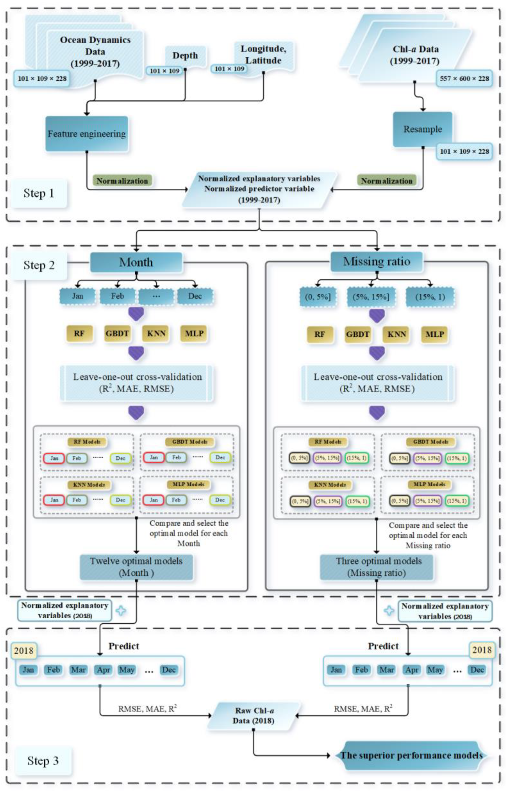
The South China Sea (SCS), our focal study region, represents the largest tropical shelf-edge sea situated in the western Pacific Ocean. It encompasses a vast expanse, covering approximately 3.56 million square kilometers. Geographically, it spans longitudinally from 0 to 23.5 degrees north and latitudinally from 99 to 122.5 degrees east.

The Chl-a concentration monthly synthetic product data, utilized as a predictor variable in this investigation (

Table 1. Description of the datasets used in the study. Chl-a, chlorophyll-a concentration; Lon, longitude; Lat, latitude; Dep, depth; WSP, wind speed; WSC, wind stress curl; SST, sea-surface temperature; TP, total precipitation; SLHF, sea-surface latent heat flux; SSHF, sea-surface sensible heat flux; LWRF, longwave radiation flux; SWRF, shortwave radiation flux; SLP, sea-level pressure.

Dataset	Unit	Min	Max	Spatial Resolution	Grid Size (Pixel)
Chl-a	mg/m3	0	26.6	0.04° × 0.04°	557 × 600 × 240
Lon	°	99	122.5	0.25° × 0.25°	101 × 109
Lat	°	0	23.5	0.25° × 0.25°	101 × 109
Dep	m	−5008	−1	0.016°×0.016°	1410 × 1409
WSP	m·s−1	1.4	15.4	0.25° × 0.25°	101 × 109 × 240
WSC	N·m−3	−2 × 10−7	2.5 × 10−7	0.25° × 0.25°	101 × 109 × 240
SST	K	285.6	304.8	0.25° × 0.25°	101 × 109 × 240
TP	m	0	0.04	0.25° × 0.25°	101 × 109 × 240
SLHF	J·m−2	−3.7 × 107	1.2 × 106	0.25° × 0.25°	101 × 109 × 240
SSHF	J·m−2	−9.8 × 106	1.4 × 106	0.25° × 0.25°	101 × 109 × 240
LWRF	W·m−2	−100.8	−15.4	0.25° × 0.25°	101 × 109 × 240
SWRF	W·m−2	57.7	293.2	0.25° × 0.25°	101 × 109 × 240
SLP	Pa	1.00 × 105	1.02 × 105	0.25° × 0.25°	101 × 109 × 240

), denoted as level 3 (version 5.0), were sourced from the Ocean Color Climate Change Initiative (OC-CCI), established by the European Space Agency (ESA) (https://www.oceancolour.org/ (accessed on 5 June 2022)). The temporal resolutions of the datasets encompassed daily, 8-day, and monthly intervals. Because of cloud cover, the high-temporal resolution datasets (daily and 8-day) had a significant amount of missing data. Moreover, in order to maintain temporal consistency between the explanatory and predictor variables, we opted to directly download and utilize the monthly Chl-a datasets for our study. The study period spanned from January 1999 to December 2018. These data combined measurements from five sensors including the Sea-Viewing Wide Field of View Sensor (SeaWiFS), the Moderate-Resolution Imaging Spectroradiometer (MODIS), the Medium-Resolution Imaging Spectroradiometer (MERIS), the Ocean and Land Colour Instrument (OLCI) sensor on the Sentinel-3A, and the Visible Infrared Imaging Radiometer (VIIRS). The selected Chl-a dataset covers the SCS from 0° N–23.5° N and 99° E–122.5° E, and its spatial coverage grid number is 557 × 600. The spatial resolution of these data is 0.04° × 0.04°, and the atmospheric correction algorithm used by the OC-CCI for the multisensor data fusion shows good adaptation to thin clouds and aerosols [32].

This study employed a range of ocean dynamics data (Table 1), all of which were gridded data, including monthly mean sea-surface temperature data, monthly mean sea-surface 10 m wind speed, monthly mean sea-surface 10 m wind stress curl, sea-surface heat flux data (comprising monthly mean surface net longwave radiation flux, monthly mean surface net shortwave radiation flux, monthly mean sensible heat flux, and monthly mean latent heat flux), total precipitation, and mean sea-level pressure. These explanatory variables in our model were obtained directly from the European Centre for Medium-Range Weather Forecasts (ECMWF) ERA-Interim dataset (http://apps.ecmwf.int/datasets/ (accessed on 5 Jun 2022)). In a study by Dee [33], it was demonstrated that ECMWF reanalysis data offered the benefit of exhibiting a closer alignment with observed data, particularly in the context of decadal scale variations. The reanalysis data utilized in this study cover the range 0° N–23.5° N, 99° E–122.5° E, with a spatial grid number of 101 × 109, as well as a spatial resolution of 0.25° × 0.25°; the time period of the study is from January 1999 to December 2018. In addition, we also used SCS depth-gridded data from the ETOPO1 global terrain model data, developed by the National Geophysical Data Center (NGDC) (https://www.ncei.noaa.gov/products/etopo-global-relief-model (accessed on 5 June 2022)), with a spatial resolution of 0.016 ° × 0.016°, and the number of spatial grids is 1410 × 1409. To ensure a consistent data resolution, we resampled the SCS depth data to a uniform grid size of 101 × 109 using cubic convolution. The datasets used in this study are shown in detail in Table 1 above.

2.2. Methodology

In Figure 1, the research flow of this paper is outlined. All of our work was centered around the imputation of Chl-a data. In the first step, we obtained some variables, which contained ocean dynamics data of the SCS from January 1999 to December 2017, depth data of the SCS, and latitude and longitude data of the SCS. We then applied feature engineering to these variables to extract and select the most relevant features as explanatory variables, which were used as input data for the models. Concurrently, similar to the approach used for the depth data, the Chl-a data for the SCS, spanning from January 1999 to December 2017, underwent resampling. Employing the cubic convolution method, we resampled the Chl-a data to align with the latitude and longitude grid points of the ocean dynamics data. This resampling was conducted at a resolution of 0.25° × 0.25°, ensuring compatibility and coherence between the two datasets. In the process of resampling the Chl-a data from high resolution to low resolution, each pixel point now represented a larger area, potentially resulting in the loss of detailed data. However, it is important to note that the spatial distribution of the Chl-a remained unchanged, and there was no alteration in the proportion of the missing data. Despite the potential loss of fine-scaled details, the overall spatial pattern and integrity of the data were preserved. Subsequently, we normalized the selected explanatory variables and the Chl-a data. This normalization process allowed for us to obtain normalized explanatory and predictor variables, facilitating a consistent and comparable framework for further analysis.

In Step 2, we recognized the substantial monthly variations in the spatiotemporal distribution of Chl-a. Simultaneously, we acknowledged that varying levels of missing data can impact the information’s completeness, influencing the efficacy of the constructed prediction models. To address these considerations, we employed classification indicators based on the month (BM) and based on the missing ratio (BMR) for the data categorization. For the BM classification, we divided the explanatory and predictor variables into 12 segments based on the corresponding month. Four machine learning methods (RF, KNN, GBDT, and MLP) were individually trained on these segmented datasets, and the optimal parameters of their models were derived using leave-one-out cross-validation. We then evaluated the models by computing performance metrics. This process yielded four sets (48 models in total), from which the optimal training model for each month was selected through a comparative analysis. Similarly, in the BMR classification, the explanatory and predictor variables were categorized into three segments based on the missing ratio. Four machine learning methods were trained on these segmented datasets, resulting in four sets (12 models in total). The optimal training model for each missing ratio scenario was then chosen through a comparative evaluation.

In Step 3, we used two approaches to predict and impute the Chl-a for 2018. First, the 12 optimal models obtained using the BM data classification approach were combined with the normalized explanatory variables for 2018 to predict Chl-a for each month of 2018 separately. We used the Chl-a raw data from 2018 as observations to compute the prediction evaluation metrics. Second, we counted the missing rate information for each month of 2018, and we used the normalized explanatory variables of 2018 as input data for the three optimal models obtained based on the BMR data classification approach to predict each month of 2018 separately according to different missing ratio. The Chl-a raw data of 2018 was also used as observations to compute the prediction evaluation metrics. Finally, a set of superior predictive models for Chl-a in SCS was obtained by comparing the performance metrics. The metrics and methods used in the study are shown below.

2.2.1. Methods for Predicting Chl-a

Multilayer Perceptron

The multilayer perceptron (MLP) stands as a variant of the feedforward neural network architecture, characterized by the inclusion of multiple hidden layers, each replete with a multitude of interconnected neurons [27,28]. Leveraging its capacity for profound nonlinear modeling, the MLP emerges as a potent tool for capturing intricate associations entwining ocean Chl-a concentration and a myriad of input features. Accomplishing this through the adept utilization of a backpropagation algorithm, the MLP optimizes the weights and biases underpinning its architecture, engendering a learning process that yields an optimal mapping that maximizes the contextual significance between the input features and the target: Chl-a concentration [4].

Random Forests

The random forest (RF) approach constitutes a methodology rooted in the realm of ensemble learning, wherein predictions are rendered through the amalgamation of numerous decision trees [34]. Each constituent decision tree is trained on a subset of randomly chosen samples, thereby introducing an element of stochasticity into the construction process. This deliberate injection of randomness serves to mitigate the model’s susceptibility to variance and bolsters the stability of its predictive outputs [14,18].

Gradient Boosted Decision Trees

Gradient Boosted Decision Trees (GBDTs) represent an iterative ensemble learning methodology, orchestrating the sequential construction of an array of decision trees, each poised to incrementally enhance predictive efficacy [29]. At every iteration, the nascent decision tree is engineered with the specific objective of rectifying the residuals stemming from the antecedent model iteration. Nevertheless, it is imperative to exercise judicious caution when navigating the domain of hyperparameter tuning during the model training process, owing to GBDT’s pronounced sensitivity to hyperparameters [28,29].

K-Nearest Neighbor

The k-nearest neighbor (KNN) method makes predictions by sample similarity. When confronted with a novel input datum, this method endeavors to identify the k most akin samples within the training corpus, subsequently extrapolating a prediction predicated upon the labels associated with this subset of samples. In the context of prognosticating oceanic Chl-a concentrations, the KNN approach emerges as particularly fitting, given its inherent capacity to account for spatial correlations [23]. This propensity stems from the inherent possibility that proximate regions within the marine milieu might exhibit akin Chl-a concentration profiles.

In this study, several distinct ML algorithms were employed to forecast Chl-a concentrations in the SCS. During the predictive process, each machine learning algorithm customizes the model’s configuration to align with the research objective, accomplished through a set of hyperparameters. Consequently, adjusting the hyperparameters of various machine learning algorithms is typically necessary during the model training phase. To acquire the most optimal prediction model, we established a range of alternative values for the hyperparameters through empirical methods. We then systematically conducted iterative assessments of the model’s predictive performance by testing it with diverse hyperparameter combinations, aiming to maximize accuracy based on R².

Table 2. Hyperparameters and alternative values for ML algorithms.

ML Algorithm	Hyperparameter	Alternative Values
MLP	hidden_layer_sizes	(100 × 1), (50 × 2), (20 × 3)
	activation	‘relu’, ‘tanh’
	solver	‘adam’, ’sgd’
	alpha	0.0001, 0.001, 0.01
RF	n_estimators	50, 100, 150
	max_depth	10, 20, 30, 40
	min_samples_split	2, 5, 10
	min_samples_leaf	1, 2, 4
GBDT	n_estimators	100, 200, 300
	learning_rate	0.01, 0.1, 0.5
	max_depth	3, 5, 7
	min_samples_split	2, 5, 10
	min_samples_leaf	1, 2, 4
KNN	k_values	3, 5, 7, 9, 11

provides a comprehensive overview of all hyperparameters and their respective alternative values utilized in this study. The selection of optimal hyperparameters was determined through rigorous leave-one-out cross validation evaluations.

2.2.2. Regression Model Accuracy Metrics

Three evaluation metrics—Root Mean Square Error (RMSE), Mean Absolute Error (MAE), and Coefficient of Determination (R²)—were employed to assess the performance of the regression models (

Table 3. Three performance metrics along with their formula.

Metrics	Formula
RMSE	$\sqrt{\frac{1}{n}{\displaystyle \sum _{i=1}^n}{(R_i-P_i)}^2}$
MAE	$\frac{1}{n}{\displaystyle \sum _{i=1}^n}\left(\left|R_i-P_i\right|\right)$
R2	$1-\frac{\sum _{i=1}^n{(R_i-P_i)}^2}{\sum _{i=1}^n{(R_i-{\overline{R}}_i)}^2}$

). The RMSE reflects the model’s sensitivity to outliers and extreme data points within the sample, while the MAE provides a measure of the potential range of errors in the estimates, offering a quantitative assessment of error.

In the provided equation, where $R_i$ represents the actual observed value of the ith pixel’s Chl-a concentration, $P_i$ stands for the predicted estimate of the ith pixel, and n represents the total number of pixel grids involved in the validation process. Additionally, ${\overline{R}}_i$ denotes the mean or average of the actual observations. R² falls within the range of 0 to 1, with higher values signifying greater accuracy. The RMSE and MAE always yield non-negative values, and values closer to zero denote a higher model accuracy. Chicco [35] contends that, when evaluating a regression model’s explanatory power, the R² is a more informative indicator than the RMSE and MAE. Consequently, in subsequent training phases, we employed R² to assess the model’s performance, while the RMSE and MAE were utilized to gauge the magnitude of the prediction errors associated with the model.

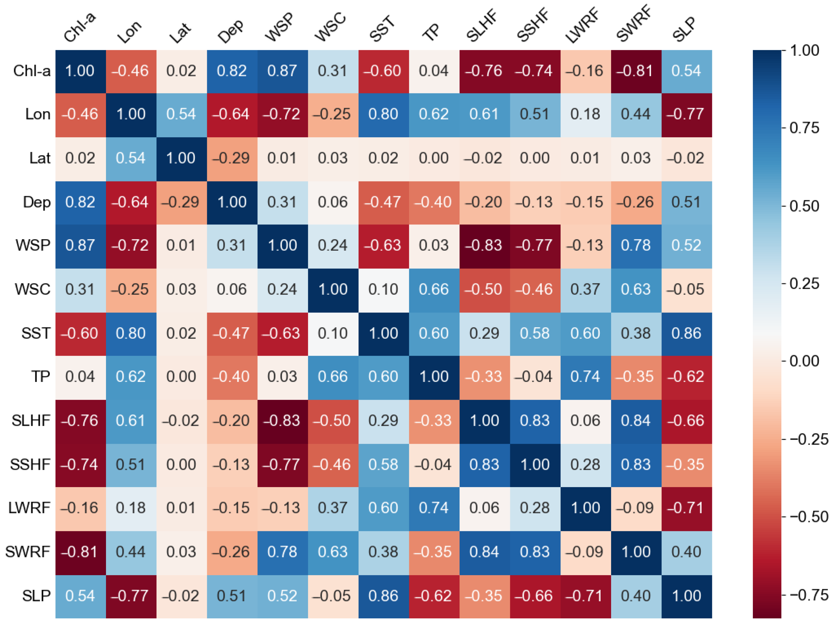
2.2.3. Determination of Explanatory Variables

Although multiple factors including monsoons, river runoff, ocean circulation, eddy, upwelling, stratification, mixing, and fronts interact to drive the spatial and temporal patterns of Chl-a [36,37,38,39,40,41], the wind and temperature have been suggested to more strongly link with the spatial and temporal variability of Chl-a in the SCS [41,42,43,44]. In addition, the spatial distribution of Chl-a in the SCS has a similar spatial consistency with the topography, presenting the characteristics of high near-shore concentration and low off-shore concentration.

Therefore, our set of influencing variables is grounded in previous research and encompasses the following components: monthly mean sea-surface temperature; monthly mean sea-surface 10 m wind speed; monthly mean sea-surface 10 m wind stress curl; monthly mean sea-surface heat flux data (including sea-surface monthly mean net longwave radiation flux, sea-surface monthly mean net shortwave radiation flux, sea-surface monthly mean sensible heat flux, and sea-surface monthly mean latent heat flux); total precipitation; mean sea-level pressure; and depth, latitude, and longitude. The spatial grid size for all of the data is 101 × 109, with a spatial resolution of 0.25° for each pixel.

Subsequently, we calculated the Pearson’s coefficients for the Chl-a data in the SCS from 1999 to 2017 with these variables. This analysis resulted in the construction of a correlation matrix plot (Figure 2). The Pearson’s correlation coefficient is a measure of the strength and direction of the linear relationship between two continuous variables, taking values between −1 and 1. A coefficient close to 1 signifies a robust positive correlation, while a value near −1 indicates a strong negative correlation. Conversely, a coefficient near 0 suggests no linear correlation.

For our study, we established a threshold at 0.7. Variables with Pearson’s coefficients greater than 0.7 or less than −0.7 were retained as explanatory variables (

Table 4. The introduction of the explanatory and predictor variables in the machine learning models, with data size expressed as the amount of real data used for training.

Variables	Data	Data Size (Pixels)
Explanatory variables	depth	26,886
	wind speed	6,130,008
	monthly mean sea-surface net shortwave radiation flux	6,130,008
	monthly mean sea-surface sensible heat flux	6,130,008
	monthly mean sea-surface latent heat flux	6,130,008
Predictor variables	Chl-a	6,130,008

). Ultimately, we identified five explanatory variables as input data for model training: depth, wind speed, monthly mean sea-surface net shortwave radiation flux, monthly mean sea-surface sensible heat flux, and monthly mean sea-surface latent heat flux. The frequency histograms of the explanatory and predictor variables are shown in Figure 3. We can observe that the depth data and Chl-a data do not follow a normal distribution. Hence, it is not appropriate to apply the z-score normalization method directly during the normalization process. To address this, we employed the min–max normalization method to normalize the depth data and used logarithmic transformation to handle the Chl-a data before applying the z-score normalization method.

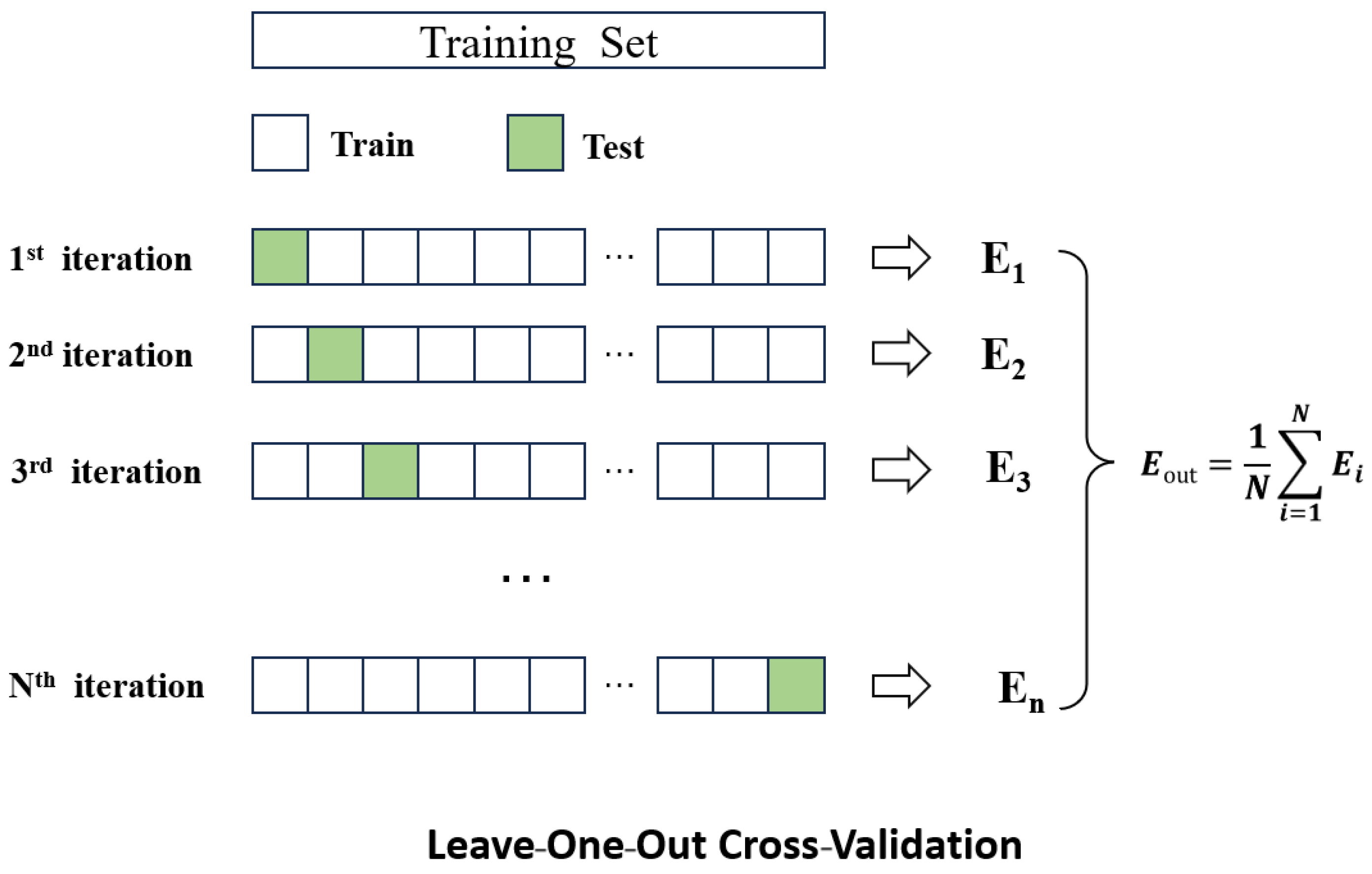
2.2.4. Cross-Validation and Parameter Tuning

We employed two imputation techniques to estimate the Chl-a concentrations in the SCS: BM imputation and BMR imputation. Additionally, we fine-tuned the model parameters through leave-one-out cross-validation. For the training and parameter tuning, we exclusively utilized data from the period spanning 1999 to 2017. Data from the year 2018 was reserved for conducting comparative tests on the final model.

During the BM imputation process, we conducted model tuning in sequential batches, each corresponding to a specific month. To illustrate, when refining the model parameters for the month of January, we gathered the Chl-a concentration data for 19 instances of January, treating each month’s data as an individual data point. Within this dataset, one data point was designated as the validation set, while the remaining data served as the training set. This procedure was repeated 19 times, with each repetition selecting a different data point as the validation set. The overall performance and stability of the model were assessed by computing the mean of the leave-one-out cross-validation performance metrics.

Moorthy’s perspective [45] suggests that missing value ratios in the range of 0–5% are generally considered inconsequential in real-world datasets and can be managed easily. However, when the missing value ratios fall within the range of 5–15%, it necessitates the use of sophisticated methods for handling and imputing missing data. Moreover, when missing value ratios exceed 15%, they can significantly impede the accuracy of predictions and inferences drawn from the data. Consequently, we categorized the data into three distinct missing value ranges based on the aforementioned criteria when employing the BMR imputation approach. In the training dataset utilized for this study, the missing ratio was as follows: 124 months falling within the 0–5% range, 74 months within the 5–15% range, and 30 months with missing values exceeding 15%. For each of these missing value ranges, we conducted parameter tuning using a leave-one-out cross-validation strategy. The detailed procedure is illustrated in Figure 4.

3. Results

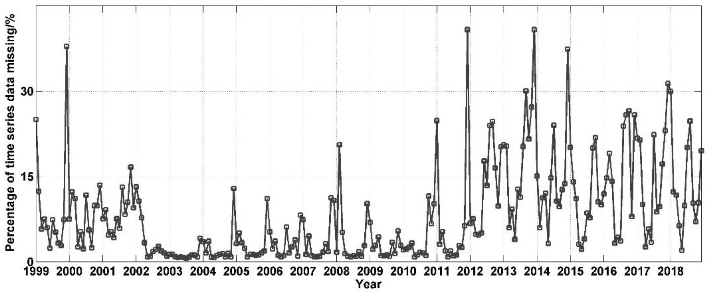
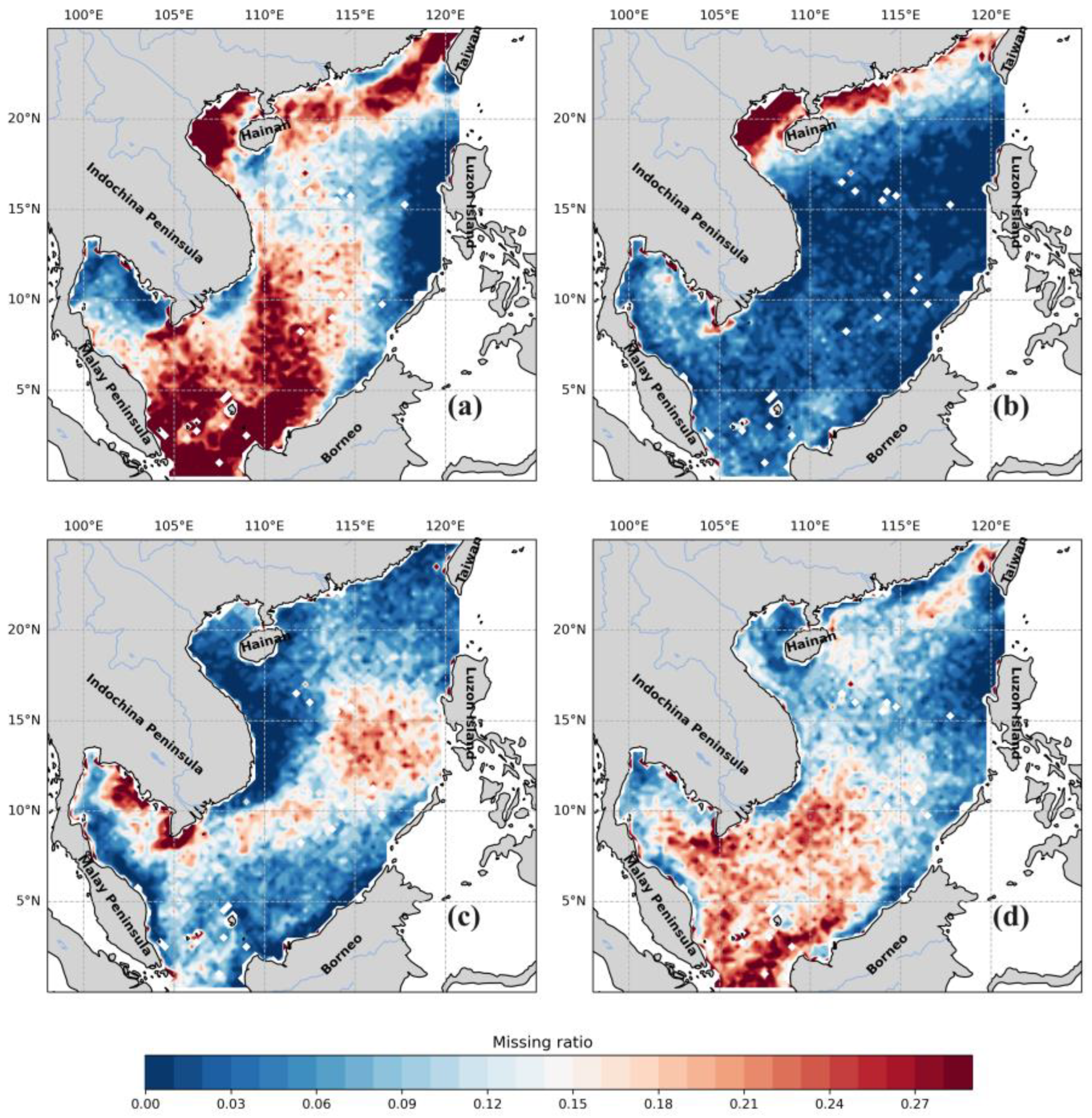
3.1. Estimation of the Total Missing in the Chl-a Data across the SCS

In this investigation, we utilized the monthly average data from the OC-CCI dataset, a composite product derived from remote sensing information gathered from multiple sources. The Chl-a dataset, following resampling, comprises a total of 11,009 grid points. This dataset exhibits temporal continuity, with individual images demonstrating a maximum grid point missing ratio of less than 40%. Notably, the winter months of each year display a relatively higher proportion of missing data in the time series. However, when assessing the data from 2002 to 2010 (Figure 5), the overall missing data ratio remain below 15%.

Geospatially, there were significant spatial differences in the missing regions of the data. Specifically, the southern region of the SCS experiences a higher incidence of missing data compared to the northern counterpart. The primary areas with substantial data gaps include the northern coast of the SCS and the Sunda shelf region within the southern part of the SCS (Figure 6).

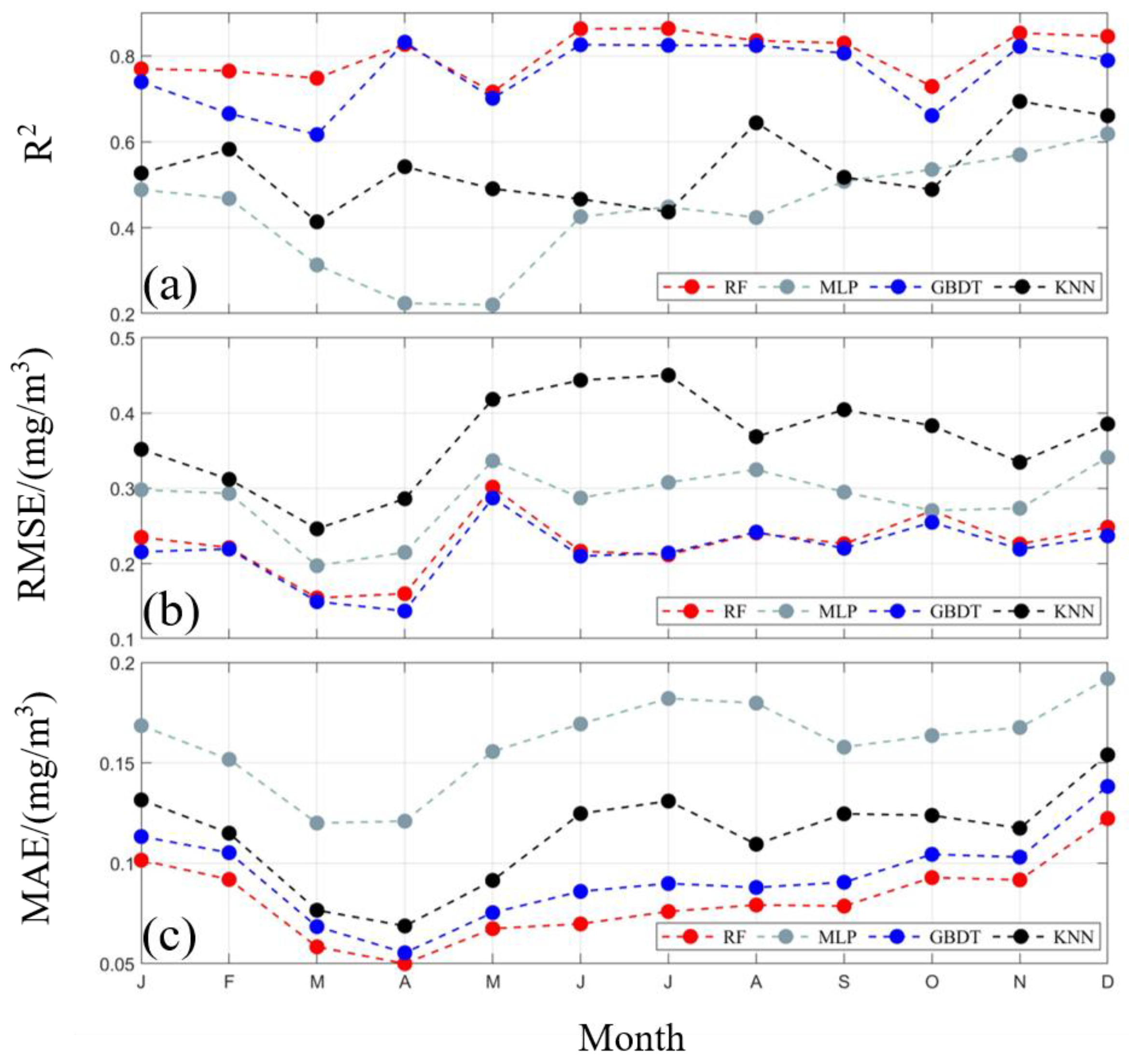
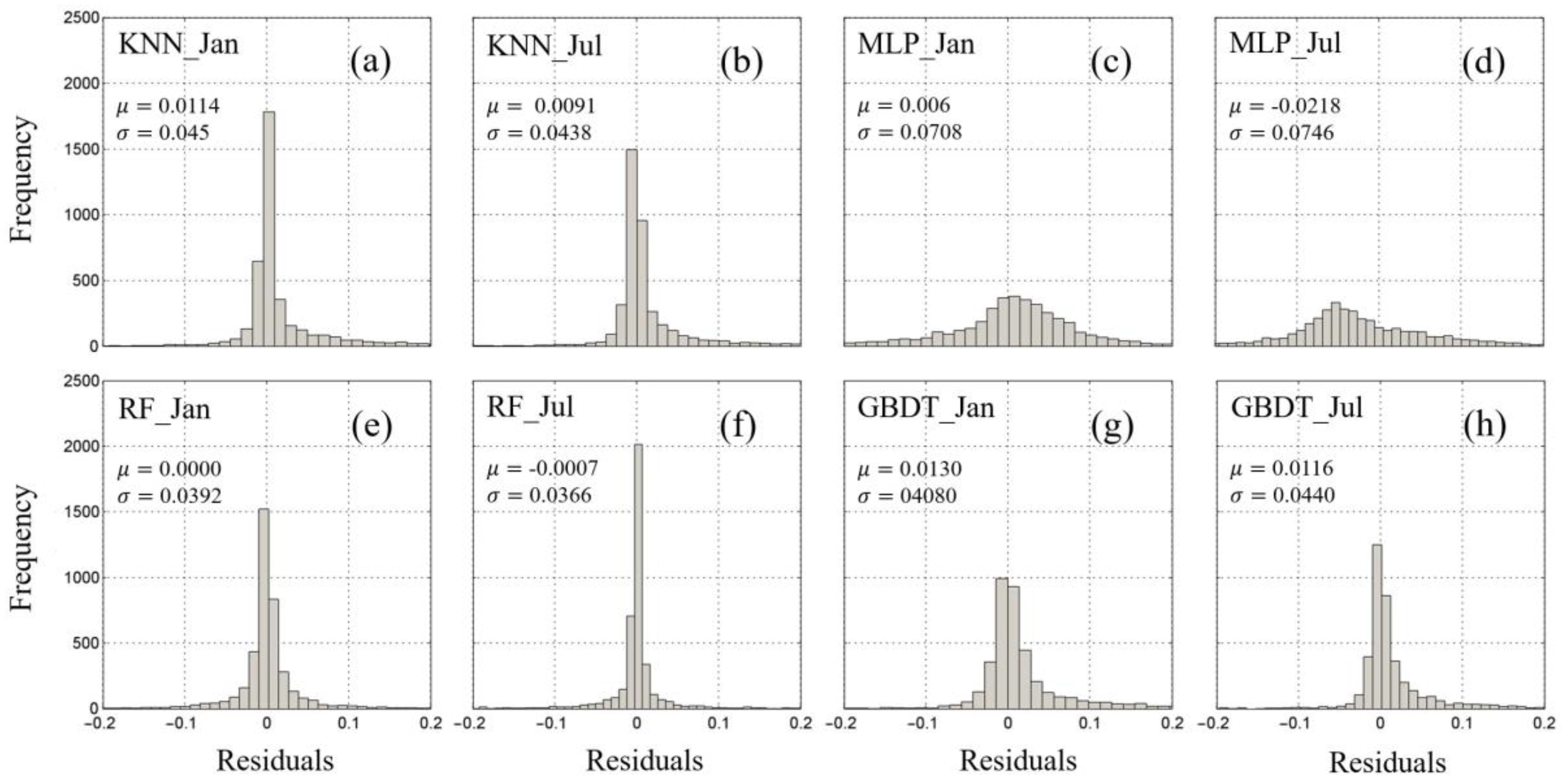
3.2. Accuracy Evaluation of Imputation Based on Month

Each month, we employed various machine learning methods to predict the Chl-a concentration in the SCS. The evaluation metrics, including MAE, RMSE, and R², were used to assess the performance of these models against the raw Chl-a concentration values (Figure 7). The monthly mean rankings for the MAE across the four methods were, consistently, as follows: RF < GBDT < KNN < MLP. Their respective MAE values were 0.08 mg/m³, 0.09 mg/m³, 0.11 mg/m³, and 0.16 mg/m³. Regarding the RMSE, the monthly mean rankings mirrored the MAE rankings: RF < GBDT < KNN < MLP, with values of 0.24 mg/m³, 0.26 mg/m³, 0.37 mg/m³, and 0.41 mg/m³, respectively. Lastly, for the R², the monthly average rankings were as follows: RF > GBDT > KNN > MLP, with corresponding values of 0.81, 0.76, 0.54, and 0.44. These consistent rankings across all three evaluation metrics highlight that the RF exhibited the lowest error and the highest prediction accuracy among the models utilized. Conversely, the MLP displayed the largest error and the lowest prediction accuracy.

To gain a more intuitive understanding of the error distributions in the imputation results from the different methods, we analyzed the prediction errors of the models by plotting the residual distributions (Figure 8). Specifically, we chose the representative months of January and July in the SCS region of 2017 in the test set for comparison. Overall, the residuals from all methods exhibited a normal distribution centered around a zero mean.

During summer, the prediction errors were observed to be more tightly concentrated within a smaller range compared to winter. The MLP prediction method displayed a relatively wider range of error distribution, primarily falling between [−0.2, 0.2]. Conversely, the errors of the other three machine learning methods concentrated within the range of [−0.1, 0.1].

Figure 8 illustrates that, both in winter and summer, the RF method demonstrated a narrower range of error distribution and exhibited a smaller root mean square error of the residuals. This indicates that the RF method is more stable compared to the other three machine learning methods, affording it distinct advantages.

3.3. Accuracy Evaluation of Imputation Based on Missing Ratio

To investigate the performance of the various machine learning algorithms in predicting the Chl-a concentration in the SCS under different scenarios of missing data, we categorized the time series data into three levels based on the missing ratios. Our aim was to evaluate the accuracy of the predictive models (

Table 5. Performance of the four machine learning models under the three missing data ratio scenarios.

Missing Ratio (%)	Evaluation Metrics	MLP	RF	GBDT	KNN
(0~5)	RMSE	0.26	0.28	0.25	0.35
	R2	0.65	0.71	0.68	0.56
	MAE	0.12	0.10	0.11	0.11
(5~15)	RMSE	0.34	0.29	0.28	0.45
	R2	0.29	0.62	0.51	0.16
	MAE	0.16	0.12	0.14	0.15
(15~)	RMSE	0.35	0.30	0.29	0.48
	R2	0.27	0.66	0.54	0.23
	MAE	0.21	0.14	0.16	0.18

). Overall, all four machine learning methods demonstrated the capability to predict Chl-a concentration in the SCS. The MAE values, both for models based on missing ratios and those based on months, followed a consistent pattern. Specifically, the predicted models exhibited the following order of the mean MAE values, RF < GBDT < KNN < MLP, corresponding to respective values of 0.12 mg/m³, 0.14 mg/m³, 0.15 mg/m³, and 0.16 mg/m³. Similarly, the RMSE analysis also showed the following order, GBDT < RF < MLP < KNN, with corresponding values of 0.27 mg/m³, 0.29 mg/m³, 0.32 mg/m³, and 0.43 mg/m³. The ordering of the mean R² values for the prediction models was RF < GBDT < MLP < KNN, with respective values of 0.66, 0.58, 0.40, and 0.31.

On the basis of the MAE and RMSE indicators, it was evident that the KNN and MLP methods exhibited larger prediction errors, while the GBDT and RF demonstrated similar prediction accuracies. At lower missing data ratios (0–5%), all four machine learning models performed comparably in terms of prediction accuracy. However, for missing ratios between 5% and 15%, as well as beyond 15%, the MLP and KNN methods exhibited inadequate predictive abilities, as their R² values hovered around 0.3. On the other hand, both the GBDT and RF methods demonstrated comparable predictions at missing ratios of 5–15% and above, with the R² values exceeding 0.5, indicating some degree of predictive capability for the Chl-a concentration in the SCS.

In contrast to the predictions of the Chl-a concentration using the BM method, we conducted an analysis to juxtapose the distribution of residuals for the winter (January) and summer (July) in the year 2017 within our test dataset (Figure 9). The residuals predicted with the various machine learning methods consistently demonstrated smaller magnitudes during the summer months when compared to the winter months. To be specific, during the winter season, the residual means followed the order RF < KNN < GBDT < MLP, while in the summer season, the order was RF < GBDT < KNN < MLP.

However, when considering the residuals predicted using these four machine learning methods while accounting for the missing ratio, we unearthed an additional compelling aspect of our analysis. While the residuals in this scenario also adhered to a normal distribution with an average value approximately centered around zero, they exhibited a broader dispersion compared to the residuals obtained through the BM imputation approach. Evidently, the variance of these residuals displayed a higher magnitude, and their overall stability appeared to be somewhat weaker than the imputation method when applied on a monthly basis, even when considering the same machine learning method and month.

This analysis not only highlights the seasonal disparities but also underscores the influence of missing data on the predictive efficacy of our models in the context of Chl-a concentration forecasting. It emphasizes the significance of comprehending not only the mean behavior but also the distribution and stability of residuals within our research.

3.4. Comparison of Spatial Imputation Based on Month and Based on Missing Ratio

When it comes to the prediction of the Chl-a concentration in the SCS, whether we approach it on a monthly basis or consider the missing ratio, it becomes evident that the RF model outperforms and exhibits greater robustness when compared to other combined machine learning models. With this in mind, we elected to make forecasts for all months of 2018 based on the month and based on the missing ratio using the RF model. Our goal was to provide a comprehensive comparison of the merits and drawbacks of these two approaches, as summarized in

Table 6. The R² for random forests predicted based on the month and predicted based on the missing ratio. RF_BM, prediction based on the month; RF_BMR, prediction based on the missing ratio; MR missing data ratio.

Month	RF_BM	RF_BMR	MR
January	0.617166	0.778624	39.87%
February	0.802298	0.692879	17.12%
March	0.587013	−0.03889	16.80%
April	0.864126	0.45351	9.8%
May	0.851278	0.739405	2.29%
June	0.863903	0.73687	15.04%
July	0.835558	0.670975	25.7%
August	0.851366	0.733656	32.59%
September	0.827067	0.76705	15.88%
October	0.744168	0.716628	10.89%
November	0.882253	0.874455	16.07%
December	0.860779	0.82279	28.13%

.

In our evaluation, we computed the R² values for the RF model in the prediction of the Chl-a concentration, using both the BM and BMR. Notably, we observed that the R² values, whether predicted based on the month or based on the missing ratio, demonstrated better performance during the latter half of 2018, while they underperformed in the initial months of the year, such as January and March. Furthermore, it is worth noting that the mean R² value for predictions made based on the month across all months was 0.80, which exceeded the mean R² value of 0.66 obtained for predictions made based on the missing ratio. This outcome underscores the superior prediction accuracy achieved by the RF model when predictions are made on a monthly basis compared to predictions based on the missing ratio. Our analysis suggests that the RF predictions made on a monthly basis offer a higher level of prediction accuracy and are, thus, preferable to predictions made by considering the missing ratio.

We employed the RF model with both the BM imputation and BMR imputation methods to analyze and compare their spatial prediction performances for the month with the highest missing Chl-a concentration data (January) and the month with the least missing Chl-a concentration data (May) in 2018. The aim was to discern the differences in their ability to capture the spatial distribution patterns of the Chl-a concentration in the SCS, as depicted in Figure 10.

In both January and May, both imputation methods—BM and BMR—displayed the capacity to reasonably depict the spatial distribution trends in the Chl-a concentration in the SCS. This entailed higher Chl-a concentrations near the shoreline and lower concentrations in the deeper basin areas, aligning closely with observations [46]. However, a more detailed examination revealed that the performance of the missing ratio-based prediction method was not as precise as that of the BM imputation. Specifically, the Chl-a concentration predicted based on the missing ratio method did not exhibit as strong a correlation with raw Chl-a data in the coastal regions compared to the BM prediction.

In winter (January), there were more obvious differences between the month-based prediction and the missing ratio prediction methods of the RF in the northern shelf of the SCS, Gulf of Tonkin, and eastern Vietnam Basin. Comparing only the northern shelf of the SCS and the Gulf of Tonkin region, the BM-imputed results were closer to the raw Chl-a; in the late spring and early summer (May), the BM predictions and the BMR predictions had a similar tendency in the sea basins region, but in the SCS coast, especially near the Gulf of Tonkin, it can be seen that the BM predictions were more closely related to the raw Chl-a data.

We generated scatter plots depicting the predictions for January and May using both the month-based and missing-ratio-based approaches, and we compared these predictions against the raw remote sensing data (Figure 11). It becomes apparent that the accuracy of the Chl-a concentration predictions in January within the SCS is notably lower than that in May, and this discrepancy is closely linked to the missing ratio of the data. Furthermore, a clear distinction arises when comparing the accuracy of the predictions based on the month versus those based on the missing ratio. The BM predictions exhibited significantly superior accuracy in both January and May.

Upon closer inspection of the scatterplot, we find that the Chl-a data are concentrated in the 0–2 mg/m³ range and that the results are biased. Figure 11a,c, with a low bias, indicate that the predictions are small, whereas Figure 11b,d, with a high bias, indicate that the predicted values are large. This is most likely related to the missing ratio of the data, where the model is biased to small predictions in the months with a large missing ratio of data, while the model is biased to large predictions in the months with a small missing ratio of data. In addition, we observed a more dispersed distribution of high data values for some Chl-a. Notably, these points were mainly concentrated in the coastal areas of the South China Sea. These coastal areas are geographically unique and distinctive, and the spatial distribution of Chl-a is not only governed by natural dynamical processes within the South China Sea, but it is also influenced by anthropogenic activities in the coastal areas.

Furthermore, we constructed frequency distribution plots illustrating the residuals obtained from both the month-based prediction method and the missing ratio prediction method of the RF for the spatially interpolating Chl-a concentration in the SCS (Figure 12). In January, it becomes evident that the residuals from both the month-based prediction method and the missing ratio prediction method exhibit a more discrete and wide-ranging distribution. In contrast, the distribution of the residuals in May appears to be relatively more concentrated. This observation suggests that predictions made with fewer missing data tend to yield smaller errors. Additionally, it is worth noting that the variance of the Chl-a concentration predicted using the month-based method is smaller than that predicted with the missing ratio method in both January and May. This implies that the results obtained using the RF method for the month-based predictions are more convergent and exhibit a higher degree of consistency. Our research outcomes underscore the distinct advantages of employing the RF month-based approach, particularly when addressing the challenges associated with high ratios of missing data, as it leads to more focused and less dispersed predictions.

4. Discussion

In comparison to prior research endeavors, this study represents a novel approach in the realm of predicting Chl-a concentration. Previous efforts have predominantly focused on constructing models that utilize satellite data in conjunction with in situ Chl-a data [11,12,13]. In contrast, our investigation explores the potential of machine learning models to predict Chl-a using ocean dynamics data. A comparative analysis reveals that certain machine learning models exhibit a commendable capability in predicting Chl-a. Among the four forecasting models examined in this study, the RF model demonstrates the highest forecasting accuracy, exhibiting a lower MAE and RMSE. Notably, this model exhibits stable performance. Following the RF model in terms of performance are the GBDT model and the KNN model. The MLP model, conversely, yields the least favorable results.

Moreover, when considering predictions based on missing data ratios, the accuracy ranking of the models remains consistent, with RF surpassing GBDT, followed by MLP and KNN. The noteworthy performance of both the RF and GBDT models can be attributed to their utilization of ensemble learning methods. These methods leverage multiple decision tree models to generate predictions, resulting in a model characterized by stable performance and superior predictive capabilities [29].

Both the RF model and GBDT model consistently outperformed the other models, whether predictions were conducted on a monthly basis or based on certainty ratios. This superior performance can be attributed to the fact that both the RF and GBDT are ensemble learning methods. These methods make predictions by amalgamating multiple decision tree models, thereby creating a model with enhanced stability and improved predictive capabilities. This approach mitigates the overfitting tendencies commonly associated with individual decision tree models, ultimately, enhancing model generalization and prediction accuracy [17]. Furthermore, during the model execution process, a leave-one-out cross-validation technique is employed on the data. This step serves to alleviate the risk of overfitting in a single model and enhances the model’s ability to generalize from the data. The RF and GBDT models exhibit strong generalization capabilities, demand less data, and are less prone to overfitting issues [16,25,28,29]. However, it is essential to note that both of these models are sensitive to parameter settings. In this study, we utilized grid search and leave-one-out cross-validation to identify the optimal model parameters.

In the prediction method based on a monthly approach, the KNN model stands out because of its simplicity, minimal parameter requirements, low computational overhead, and relatively balanced results with low error variance [23]. Nevertheless, its R² is relatively small, suggesting that the model’s predictive performance exhibits some instability. On the other hand, the MLP model is sensitive to both data volume and sample distribution [28]. When the data volume is insufficient or the sample distribution is imbalanced, the MLP model may struggle to generalize effectively to new data. In the context of monthly predictions, the spatial modal distributions for all months appear similar, featuring limited data points with high Chl-a concentration values and a preponderance of data points with low Chl-a concentration values. Consequently, this results in a suboptimal overall performance and diminished generalization. Conversely, when predicting based on the missing ratio approach, the inherent imbalance in the distribution of the Chl-a concentration data values in the SCS is mitigated. This leads to an improvement in the prediction accuracy for the MLP model. Thus, the performance of the MLP model is enhanced when utilizing the missing ratio method for prediction. Generally speaking, while the KNN model offers simplicity and efficiency, its monthly predictions exhibit some instability. In contrast, the MLP model’s performance is closely tied to the data volume and distribution, and its efficacy improves when predicting according to the missing ratio approach, which helps balance the distribution of the missing Chl-a data in the SCS. When we constructed models based on missing ratios, because each pixel is relatively independent, the main difference between images with high missing ratios and those with fewer missing ratios is the number of samples trained. More pixels will be lost in the SCS during the rainy season (because of cloud cover) than during the dry season, so it is reasonable to believe that the ratios of missing pixels may be an index of climate. Therefore, in future studies of Chl-a imputation in the SCS, the inclusion of a climate factor may be an important contribution to model improvement.

In addition to the above prediction methods, deep learning is also known to perform well in the prediction of Chl-a [47], and it is able to find abstract and nonlinear relationships in the research object. The large number of explanatory variables used in this study may also have good potential if deep learning methods are used. However, deep learning usually requires more computational resources, including GPUs, and machine learning algorithms may perform better with relatively low computational resources. Therefore, the advantages and disadvantages of these two approaches for Chl-a prediction in the South China Sea are yet to be investigated in our further comparative study.

In this research paper, we investigated the application of four distinct machine learning methods for interpolating Chl-a concentration data spanning from 1999 to 2018. Our analysis reveals that the RF model offers a more convenient and accurate means of obtaining long-term spatial distribution data for Chl-a concentrations. This capability proves invaluable for comprehending the spatiotemporal patterns of Chl-a concentration changes. It is imperative to acknowledge that numerous factors contribute to the spatial and temporal variations in Chl-a concentrations. These factors encompass spatial positioning, seasonal fluctuations, physicochemical properties of seawater, and biological factors, as well as natural elements like meteorological conditions, hydrology, ocean currents, and atmospheric patterns. Additionally, anthropogenic factors such as maritime zoning, land-based discharges, and coastal infrastructure also play a significant role [48]. Given the accessibility of data and the suitability of our methodology, we exclusively utilized ocean dynamics data as indicator variables in this study. In future investigations, we intend to incorporate a broader spectrum of data sources to assess the predictive capabilities of different models comprehensively. Furthermore, we plan to delve into a detailed examination of the uncertainty associated with machine learning imputation methods. This will enhance our understanding of the robustness and limitations of these techniques for Chl-a concentration imputation.

5. Conclusions

In this study, we used an innovative approach that combines ocean dynamics datasets with multiple machine learning algorithms to predict Chl-a in the South China Sea. The study was centered around four distinct predictive models: RF, GBDT, KNN, and MLP. These models were trained using monthly temporal resolution data, employing two distinct training approaches: prediction based on the month and prediction based on the missing data ratio. The optimal model parameters were determined through grid search and validated using leave-one-out cross-validation, with test data utilized for validation purposes. The evaluation of the model performance was based on key metrics including R², RMSE, and MAE. The study’s findings are summarized as follows:

(1)

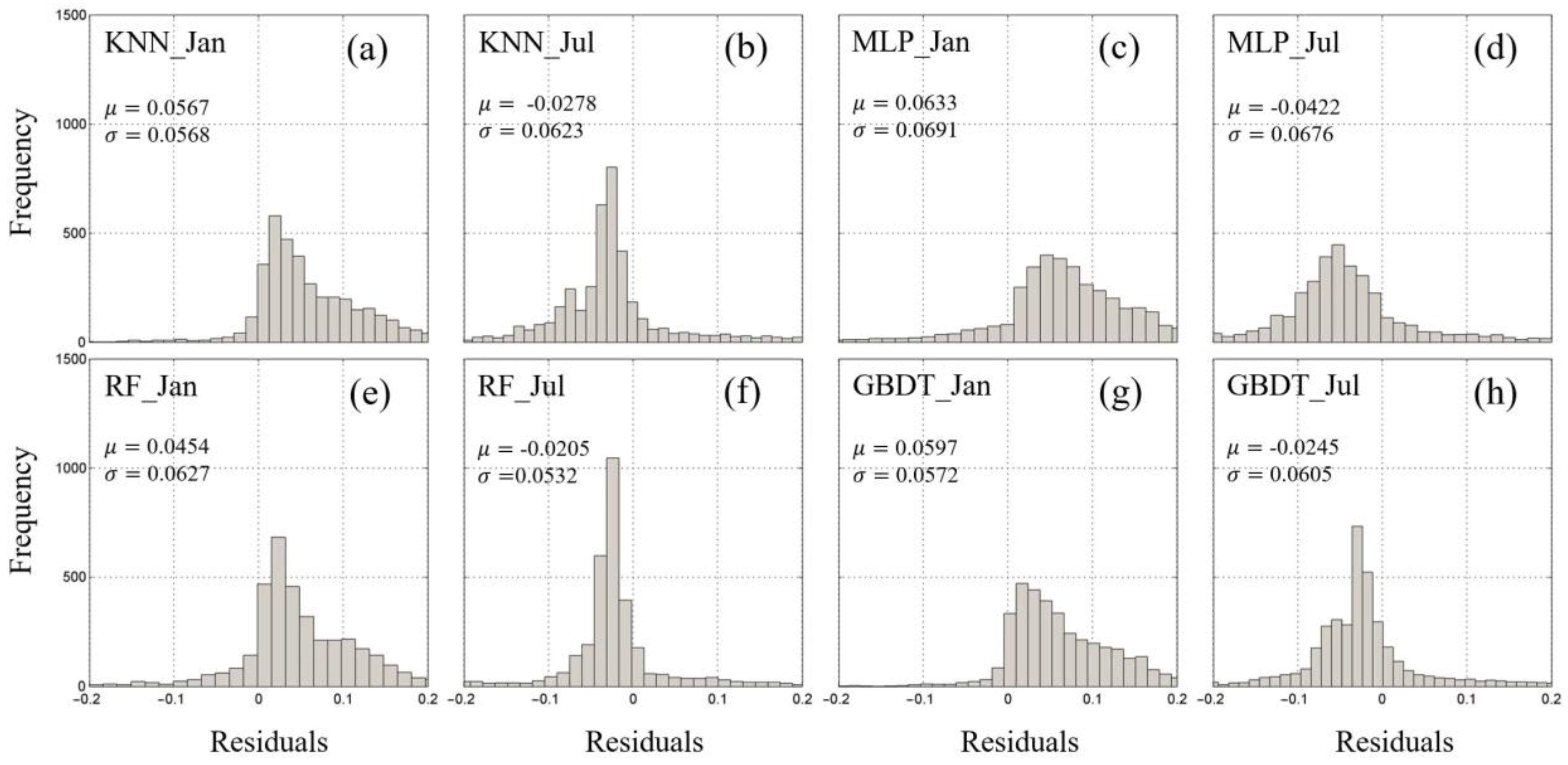
Among the models employing the monthly prediction approach, the RF model consistently demonstrated the highest prediction accuracy, followed by GBDT and KNN, with the MLP performing the least favorably. The RF model excels in both prediction accuracy and the distribution of model residuals when compared to the other models.

(2)

In the case of models employing the missing ratio approach, the RF model again emerged as the most accurate, followed by GBDT and MLP, while KNN lagged behind with a comparatively poorer combined performance. It is important to note that the overall prediction accuracy decreased as the data’s missing ratio increased.

(3)

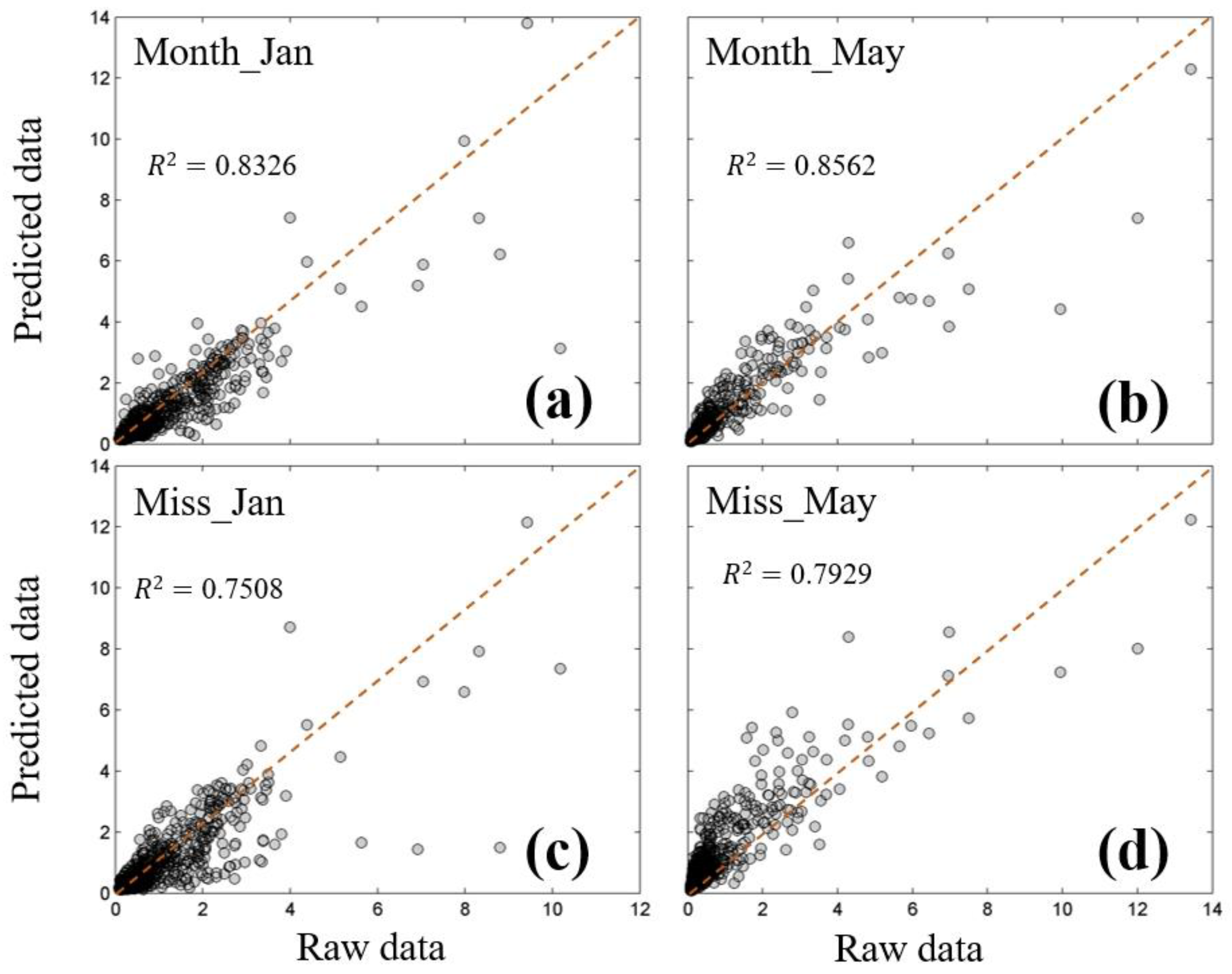
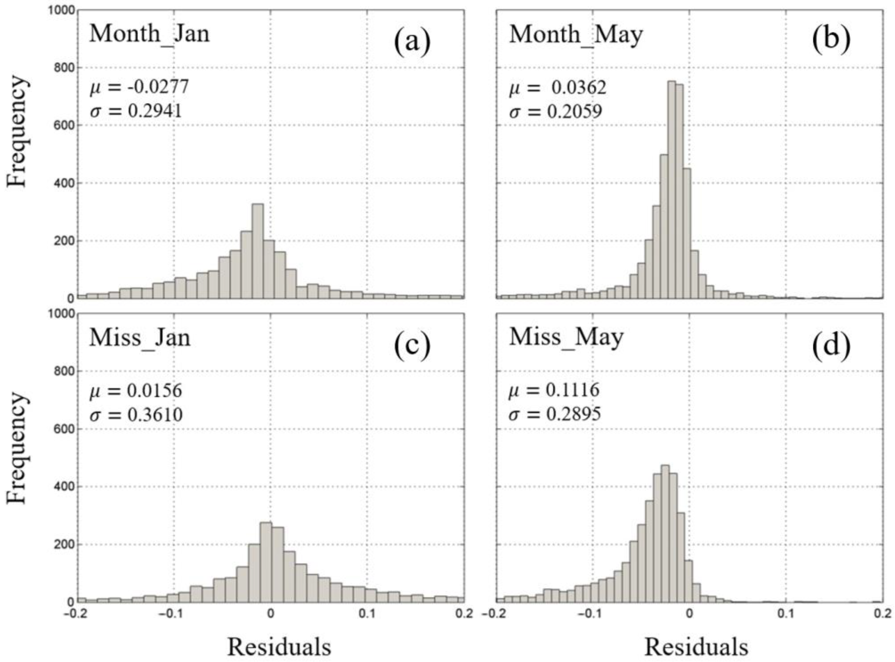
Irrespective of the prediction approach, the RF model consistently delivered a superior performance. When comparing the two prediction methods within the RF model using 2018 data, it became apparent that increasing the missing data ratios negatively impacted the accuracy of the monthly prediction approach. In general, the results obtained through the monthly prediction approach exhibited a better overall accuracy, more stable residual variances, and superior generalization capabilities compared to the missing ratio prediction approach.

Therefore, based on these findings, we recommend the utilization of the RF model for future Chl-a concentration forecasting in the SCS. This model consistently demonstrates robust performance, making it a reliable choice for accurate and stable predictions in this context.

References

1. Donders, A.; van der Heijden, G.; Stijnen, T.; Moons, K. Review: A gentle introduction to imputation of missing values. J. Clin. Epidemiol. 2006, 59, 1087–1109. [Google Scholar] [CrossRef]
2. Dakos, V.; Matthews, B.; Hendry, A.; Levine, J.; Loeuille, N.; Norberg, J.; Nosil, P.; Scheffer, M.; Meester, L. Ecosystem tipping points in an evolving world. Nat. Ecol. Evol. 2019, 3, 355–362. [Google Scholar] [CrossRef]
3. Wang, F.; Li, X.; Tang, X.; Sun, X.; Zhang, J.; Yang, D.; Xu, L.; Zhang, H.; Yuan, H.; Wang, Y. The seas around China in a warming climate. Nat. Rev. Earth Environ. 2023, 4, 535–551. [Google Scholar] [CrossRef]
4. Kajiyama, T.; D’Alimonte, D.; Cunha, J. Performance prediction of ocean color Monte Carlo simulations using multi-layer perceptron neural networks. Pro. Com. Sci. 2011, 4, 2186–2195. [Google Scholar] [CrossRef]
5. Amorim, F.; Rick, J.; Lohmann, G.; Wiltshire, K. Evaluation of Machine Learning Predictions of a Highly Resolved Time Series of Chlorophyll-a Concentration. Appl. Sci. 2021, 11, 7208. [Google Scholar] [CrossRef]
6. Jin, D.; Lee, E.; Kwon, K.; Kim, T. Deep Learning Model Using Satellite Ocean Color and Hydrodynamic Model to Estimate Chlorophyll-a Concentration. Remote Sens. 2021, 13, 2003. [Google Scholar] [CrossRef]
7. Im, G.; Lee, D.; Lee, S.; Lee, J.; Lee, S.; Park, J.; Heo, T. Estimating Chlorophyll-a Concentration from Hyperspectral Data Using Various Machine Learning Techniques: A Case Study at Paldang Dam, Republic of Korea. Water 2022, 14, 4080. [Google Scholar] [CrossRef]
8. González-Enrique, J.; Ruiz-Aguilar, J.; Madrid Navarro, E.; Martínez Álvarez-Castellanos, R.; Felis Enguix, I.; Jerez, J.; Turias, I. Deep Learning Approach for the Prediction of the Concentration of Chlorophyll a in Seawater. A Case Study in El Mar Menor (Spain). In Proceedings of the 17th International Conference on Soft Computing Models in Industrial and Environmental Applications (SOCO 2022): Lecture Notes in Networks and Systems, Salamanca, Spain, 5–7 September 2022; pp. 72–85. [Google Scholar]
9. Liu, M.; Liu, X.; Ma, A.; Li, T.; Du, Z. Spatio-temporal stability and abnormality of chlorophyll-a in the northern south china sea during 2002–2012 from modis images using wavelet analysis. Cont. Shelf. Res. 2014, 75, 15–27. [Google Scholar] [CrossRef]
10. Kutser, T. Passive optical remote sensing of cyanobacteria and other intense phytoplankton blooms in coastal and inland waters. Int. J. Remote Sens. 2009, 30, 4401–4425. [Google Scholar] [CrossRef]
11. Kown, Y.; Baek, S.; Lim, Y.; Pyo, J.; Ligaray, M.; Park, Y.; Cho, K. Monitoring Coastal Chlorophyll-a Concentrations in Coastal Areas Using Machine Learning Models. Water 2018, 10, 1020. [Google Scholar] [CrossRef]
12. Watanabe, F.; Alcntara, E.; Rodrigues, T.; Rotta, L.; Bernardo, N.; Imai, N. Remote sensing of the chlorophyll-a based on OLI/Landsat-8 and MSI/Sentinel-2A (Barra Bonita reservoir, Brazil). An. Da Acad. Bras. De Ciências 2018, 90, 1987–2000. [Google Scholar] [CrossRef]
13. Mattei, F.; Scardi, M. Mining satellite data for extracting chlorophyll a spatio-temporal patterns in the Mediterranean Sea. Environ. Modell. Softw. 2022, 150, 105353. [Google Scholar] [CrossRef]
14. Mohebzadeh, H.; Mokari, E.; Daggupati, P.; Biswas, A. A machine learning approach for spatiotemporal imputation of MODIS chlorophyll-a. Int. J. Remote Sens. 2021, 42, 7381–7740. [Google Scholar] [CrossRef]
15. Wang, S.; Li, W.; Hou, S.; Guan, J.; Yao, J. STA-GAN: A Spatio-Temporal Attention Generative Adversarial Network for Missing Value Imputation in Satellite Data. Remote Sens. 2022, 15, 88. [Google Scholar] [CrossRef]
16. Chen, S.; Hu, C.; Barnes, B.; Xie, Y.; Lin, G.; Qiu, Z. Improving ocean color data coverage through machine learning. Remote Sens. Environ. 2019, 222, 286–302. [Google Scholar] [CrossRef]
17. Yu, P.; Gao, R.; Zhang, D.; Liu, Z. Predicting coastal algal blooms with environmental factors by machine learning methods. Ecol. Indic. 2021, 12, 107334. [Google Scholar] [CrossRef]
18. Kim, W.; Cho, W.; Choi, J.; Kim, J.; Park, C.; Choo, J. A Comparison of the Effects of Data Imputation Methods on Model Performance. In Proceedings of the International Conference on Advanced Communications Technology, PyeongChang, Republic of Korea, 17–20 February 2019; pp. 592–599. [Google Scholar]
19. Wongoutong, C. Imputation Methods in Time Series with a Trend and a consecutive missing value pattern. Thail. Statist. 2021, 19, 866–879. [Google Scholar]
20. Janik, M.; Bossew, P.; Kurihara, O. Machine learning methods as a tool to analyse incomplete or irregularly sampled radon time series data. Sci. Total Environ. 2018, 630, 1155–1167. [Google Scholar] [CrossRef]
21. Kim, J.; Shin, J.; Lee, H.; Lee, D.; Kang, J.; Cho, K.; Lee, Y.; Chon, K.; Baek, S.; Park, Y. Improving the performance of machine learning models for early warning of harmful algal blooms using an adaptive synthetic sampling method. Water Res. 2021, 207, 11782. [Google Scholar] [CrossRef]
22. He, Q.; Wang, M.; Liu, K. Spatial interpolation of temperature elements based on machine learning. Plateau Meteorol. (Chin.) 2022, 41, 16. [Google Scholar]
23. Poloczek, J.; Treiber, N.; Kramer, O. KNN Regression as Geo-Imputation Method for Spatio-Temporal Wind Data. In Proceedings of the International Joint Conference SOCO’14-CISIS’14-ICEUTE’14, Bilbao, Spain, 25–27 June 2014; pp. 185–193. [Google Scholar]
24. Thomas, T.; Rajabi, E. A systematic review of machine learning-based missing value imputation techniques. Data Technol. Appl. 2021, 55, 558–585. [Google Scholar] [CrossRef]
25. Kim, H.; Soh, H.; Kwak, M.; Han, S. Machine Learning and Multiple Imputation Approach to Predict Chlorophyll-a Concentration in the Coastal Zone of Korea. Water 2022, 14, 1862. [Google Scholar] [CrossRef]
26. Lin, J.; Liu, Q.; Song, Y.; Liu, J.; Yin, Y.; Hall, N. Temporal Prediction of Coastal Water Quality Based on Environmental Factors with Machine Learning. J. Mar. Sci. Eng. 2023, 11, 1608. [Google Scholar] [CrossRef]
27. Jerez, J.; Molina, I.; García-Laencina, P.; Alba, E.; Ribelles, N.; Martín, M.; Franco, L. Missing data imputation using statistical and machine learning methods in a real breast cancer problem. Artif. Intell. Med. 2010, 50, 105–115. [Google Scholar] [CrossRef]
28. Nunes Carvalho, T.; Lima Neto, I.; Souza Filho, F. Uncovering the influence of hydrological and climate variables in chlorophyll-A concentration in tropical reservoirs with machine learning. Environ. Sci. Pollut. Res. 2022, 29, 74967–74982. [Google Scholar] [CrossRef]
29. Hu, M.; Wang, Y.; Sun, Z.; Su, Y.; Li, S.; Bao, Y.; Wen, J. Performance of ensemble-learning models for predicting eutrophication in Zhuyi Bay, Three Gorges Reservoir. River Res. Appl. 2020, 37, 1104–1114. [Google Scholar] [CrossRef]
30. Shin, Y.; Kim, T.; Hong, S.; Lee, S.; Lee, E.; Hong, S.; Lee, C.; Kim, T.; Park, M.S.; Park, J. Prediction of Chlorophyll-a Concentrations in the Nakdong River Using Machine Learning Methods. Water 2020, 12, 1822. [Google Scholar] [CrossRef]
31. Feng, L.; Nowak, G.; O’Neill, T.; Welsh, A. CUTOFF: A spatio-temporal imputation method. J. Hydrol. 2014, 519, 3591–3605. [Google Scholar] [CrossRef]
32. Sathyendranath, S.; Brewin, R.; Brockmann, C.; Brotas, V.; Calton, B.; Chuprin, A.; Cipollini, P.; Couto, A.; Dingle, J.; Doerffer, R. An Ocean-Colour Time Series for Use in Climate Studies: The Experience of the Ocean-Colour Climate Change Initiative (OC-CCI). Sensors 2019, 19, 4285. [Google Scholar] [CrossRef]
33. Dee, D.; Uppala, S.; Simmons, A.; Berrisford, P.; Poli, P.; Kobayashi, S.; Andrae, U.; Balmaseda, M.; Balsamo, G.; Bauer, P. The ERA-Interim reanalysis: Configuration and performance of the data assimilation system. Q. J. Roy. Meteor. Soc. 2011, 137, 553–597. [Google Scholar] [CrossRef]
34. Belgiu, M.; Drăguţ, L. Random forest in remote sensing: A review of applications and future directions. Isprs J. Photogramm. 2016, 114, 24–31. [Google Scholar] [CrossRef]
35. Chicco, D.; Warrens, M.; Jurman, G. The coefficient of determination R-squared is more informative than SMAPE, MAE, MAPE, MSE and RMSE in regression analysis evaluation. Peerj Comput. Sci. 2021, 7, e623. [Google Scholar] [CrossRef] [PubMed]
36. Lin, P.; Ma, J.; Chai, F.; Xiu, P.; Liu, H. Decadal variability of nutrients and biomass in the southern region of Kuroshio Extension. Prog. Oceanogr. 2020, 188, 102441. [Google Scholar] [CrossRef]
37. Yu, Y.; Wang, Y.; Cao, L.; Tang, R.; Chai, F. The ocean-atmosphere interaction over a summer upwelling system in the South China Sea. J. Mar. Syst. 2020, 208, 103360. [Google Scholar] [CrossRef]
38. Xiu, P.; Chai, F. Eddies Affect Subsurface Phytoplankton and Oxygen Distributions in the North Pacific Subtropical Gyre. Geophys. Res. Lett. 2020, 47, e2020GL087037. [Google Scholar] [CrossRef]
39. Guo, L.; Xiu, P.; Chai, F.; Xue, H.; Wang, D.; Sun, J. Enhanced Chlorophyll Concentrations Induced by Kuroshio Intrusion Fronts in the Northern South China Sea. Geophys. Res. Lett. 2017, 44, 11–565. [Google Scholar] [CrossRef]
40. Guo, M.; Xiu, P.; Li, S.; Chai, F.; Xue, H.; Zhou, K.; Dai, M. Seasonal variability and mechanisms regulating chlorophyll distribution in mesoscale eddies in the South China Sea. J. Geophys. Res.-Ocean. 2017, 122, 5329–5347. [Google Scholar] [CrossRef]
41. Palacz, A.P.; Xue, H.; Armbrecht, C.; Zhang, C.; Chai, F. Seasonal and inter-annual changes in the surface chlorophyll of the South China Sea. J. Geophys. Res. 2011, 116, C09015. [Google Scholar] [CrossRef]
42. Liu, M.; Liu, X.; Ma, A.; Zhang, B.; Jin, M. Spatiotemporal variability of chlorophyll a and sea surface temperature in the northern south china sea from 2002 to 2012. Can. J. Remote Sens. 2015, 41, 547–560. [Google Scholar] [CrossRef]
43. Yu, Y.; Xing, X.; Liu, H.; Yuan, Y.; Wang, Y.; Chai, F. The variability of chlorophyll-a and its relationship with dynamic factors in the basin of the South China Sea. J. Mar. Syst. 2019, 200, 103230. [Google Scholar] [CrossRef]
44. Wang, T.; Sun, Y.; Su, H.; Lu, W. Declined trends of chlorophyll a in the South China Sea over 2005–2019 from remote sensing reconstruction. Acta Oceanol. Sin. 2023, 42, 12–24. [Google Scholar] [CrossRef]
45. Moorthy, K.; Mohamad, M.; Deris, S. A Review on Missing Value Imputation Algorithms for Microarray Gene Expression Data. Curr. Bioinform. 2014, 9, 18–22. [Google Scholar] [CrossRef]
46. Li, A.; Feng, Y.; Wang, Y.; Xue, H. Spatial and temporal changes of water area with high chlorophyll concentration in the South China Sea based on OC-CCI data. J. Trop. Ocean. (Chin.) 2022, 41, 13. [Google Scholar]
47. Liu, N.; Chen, S.; Chen, Z.; Wang, X.; Xiao, Y.; Li, X.; Gong, Y.; Wang, T.; Zhang, X.; Liu, S. Long-term prediction of sea surface chlorophyll-a concentration based on the combination of spatio-temporal features. Water Res. 2022, 211, 118040. [Google Scholar]
48. Blondeau-Patissier, D.; Gower, J.; Dekker, A.; Phinn, S.; Brando, V. A review of ocean color remote sensing methods and statistical techniques for the detection, mapping and analysis of phytoplankton blooms in coastal and open oceans. Prog. Oceanogr. 2014, 123, 123–144. [Google Scholar] [CrossRef]
Figure 1. Flowchart of the machine learning approach to reconstructing SCS Chl-a concentrations.
Jmse 12 00013 g001
Figure 2. Correlation analysis of the explanatory and predictor variables: Pearson’s correlation matrix plot. Chl-a, chlorophyll-a concentration; Lon, longitude; Lat, latitude; Dep, topography; WSP, wind speed; WSC, wind stress curl; SST, sea-surface temperature; TP, total precipitation; SLHF, sea-surface latent heat flux; SSHF, sea-surface sensible heat flux; LWRF, longwave radiation flux; SWRF, shortwave radiation flux; SLP, sea-level pressure.
Jmse 12 00013 g002
Figure 3. Frequency histograms of the explanatory and predictor variables: (a) log10(Chl-a); (b) depth; (c) monthly mean sea-surface latent heat flux; (d) monthly mean sea-surface sensible heat flux; (e) monthly mean sea-surface net shortwave radiation flux; (f) wind speed.
Jmse 12 00013 g003
Figure 4. Schematic diagram of the leave-one-out cross-validation method.
Jmse 12 00013 g004
Figure 5. Time series of Chl-a concentration missing ratios in the SCS.
Jmse 12 00013 g005
Figure 6. Spatial variations in the Chl-a concentration missing ratios across seasons in the SCS: (a) spring; (b) summer; (c) autumn; (d) winter.
Jmse 12 00013 g006
Figure 7. Validation of the spatial imputation results for the monthly mean Chl-a concentration in the SCS: (a) R2; (b) RMSE; (c) MAE.
Jmse 12 00013 g007
Figure 8. Frequency distributions of the residual Chl-a concentration in the SCS region interpolated based on the month for the four machine learning methods: (a) KNN in January; (b) KNN in July; (c) MLP in January; (d) MLP in July; (e) RF in January; (f) RF in July; (g) GBDT in January; (h) GBDT in July. μ, mean; σ, standard deviation.
Jmse 12 00013 g008
Figure 9. Frequency distributions of the Chl-a concentration residuals in the SCS region interpolated based on the missing ratio for the four machine learning methods: (a) KNN in January; (b) KNN in July; (c) MLP in January; (d) MLP in July; (e) RF in January; (f) RF in July; (g) GBDT in January; (h) GBDT in July. μ, mean; σ, standard deviation.
Jmse 12 00013 g009
Figure 10. Spatial distribution of the RF model predictions of the Chl-a concentration in the South China Sea based on the month method and based on the missing ratio method: (a) Chl-a raw data of January 2018; (b) prediction results of RF based on the month in January 2018; (c) prediction results of RF based on the missing ratio in January 2018; (d) Chl-a raw data of May 2018; (e) prediction results of RF based on the month in May 2018; (f) prediction results of RF based on the missing ratio in May 2018.
Jmse 12 00013 g010
Figure 11. Scatter plots of the monthly mean Chl-a concentrations from satellite data versus monthly mean Chl-a concentrations RF model predicted based on the month and based on the missing ratio in January and May 2018: (a) January based on the month; (b) May based on the month; (c) January based on the missing ratio; (d) May based on the missing ratio.
Jmse 12 00013 g011
Figure 12. Frequency distributions of the residuals from the RF methods for the spatial imputation of the Chl-a concentrations in the SCS: (a,b) predicted based on the month; (c,d) predicted based on the missing ratio. μ, mean; σ, standard deviation.
Jmse 12 00013 g012