Environmental Parameters Related to Hypoxia Development and Persistence in Jinhae Bay from 2011 to 2016 and Their Potential for Hypoxia Prediction

Abstract

Jinhae Bay, a semi-enclosed bay on the southern coast of Korea, is a major aquaculture area that forms a spawning ground and nursery for commercially important fishes. Since the late 1960s, industrial and domestic waste from adjacent cities and industrial complexes has been released into the region, resulting in chronic hypoxia and red tides. As a central site of environmental monitoring efforts for aquaculture and fisheries in southeastern Korea, Jinhae Bay was surveyed every 2 months usually, and every 2–3 weeks during the hypoxia season, with the seawater properties observed at approximately 31–34 stations. The maximum area and duration of hypoxia in Jinhae Bay occurred in 2016 (316 km² and 26 weeks, respectively), with minima of area in 2013 (213 km²) and duration in 2011 (15 weeks). Correlation analyses of the seawater properties, weather parameters, and hypoxia indices showed that the hypoxic area was positively correlated with the surface-water temperature, air temperature, and rainfall; the minimum dissolved oxygen concentrations were negatively correlated with the air and water temperatures and bottom-water nutrient levels; and the water stability was negatively correlated with the surface-water salinity and positively correlated with both the surface- and bottom-water nitrate and silicate concentrations. These findings imply that the air temperature and precipitation may be important factors in the development and persistence of hypoxia in Jinhae Bay via the control of the stratification intensity and eutrophication of the water column. Therefore, we tested these parameters for their potential to predict hypoxia. Based on our results, we propose the following trends of hypoxia in Jinhae Bay: the initial hypoxia development generally depends on the criteria of an air temperature ≥ 19.5 °C for 1 week and total precipitation > 100 mm over 4 weeks, and it becomes more severe (≥50% coverage) under strong eutrophication, mainly due to organic matter discharge following heavy rainfall, based on the logarithmic correlation with the 4-week rainfall (R² = 0.6). Therefore, the hypoxic area index can be predicted using its linear regression relationships with the 1-week air temperature and 4-week precipitation (R² = 0.56). This study tested the prediction of the hypoxic area based on a simple calculation method and weather parameter criteria, and it demonstrated the potential of this method for precisely forecasting hypoxia in combination with biogeochemical models or other mathematical solutions to prevent massive fishery damage.

1. Introduction

Hypoxia refers to a state in which the dissolved oxygen (DO) concentration in a water body is sufficiently low to threaten the health of the aquatic ecosystem. Numerous studies have aimed to quantify the threshold concentrations for defining hypoxic conditions based on chemical and biological responses to changes in the DO concentration [1,2,3]. A previous study found that the DO concentration ranges affecting the growth and metabolism of marine fauna in a coastal region were 6.4–8.6 mg/L and 2.9–5.7 mg/L, respectively, whereas DO concentrations of 0.7–2.9 mg/L resulted in the death of marine life [1]. In another study, nekton migrated to other regions when the DO concentration was ≤5.7 mg/L; DO concentrations ≤ 4.3 mg/L were associated with shellfish mortality, and almost all marine species were impacted at DO concentrations ≤ 2.9 mg/L [2]. The threshold DO concentration at which organisms are threatened is generally between 2.9 and 3.6 mg/L; however, a chemical concentration standard for hypoxia of 2.0 mg/L is commonly used [4,5,6].

Over 400 coastal regions are hypoxic worldwide [7], and the development of hypoxia is commonly observed in regions with abundant anthropogenic activities. Representative hypoxic coastal regions include the Baltic Sea, the Gulf of Mexico, and Chesapeake Bay; among Asian waters, hypoxia is frequently observed in Tokyo Bay and Ise Bay in Japan, as well as in the southern coastal waters of South Korea, including Jinhae Bay and Gamak Bay.

The development of hypoxia is a consequence of complex interactions among multiple environmental factors that can be categorized into physical (processes preventing oxygen supply) and biogeochemical (processes consuming oxygen) factors, with stratification and eutrophication (nutrient loading) being representative factors supporting hypoxia development in coastal areas. Stratification, a steep density gradient between surface and bottom waters, hinders the vertical exchange of water, affecting the oxygen supply to the bottom water and resulting in hypoxia [8,9]. Eutrophication, the enrichment of inorganic or organic nutrients, leads to increased oxygen consumption for the degradation of organic matter in both the water column and sediment, resulting in hypoxia.

For example, depending on the environmental characteristics of the studied sea, researchers have suggested that physical factors such as stratification are the primary drivers of hypoxia [10,11,12]. Alternatively, some researchers have stated that the inflow of nutrients such as N and P is the major cause of hypoxia [13,14,15,16]. In Tokyo Bay, hypoxic bottom water during summer was attributed mainly to coastal circulation driven by the salinity difference between freshwater and seawater and stratification caused by increased surface-water temperatures [10]. However, in the Gulf of Mexico, a 50–60% nitrate load reduction was required to reduce the hypoxic area to <5000 km², suggesting that increasing nitrate fluxes from the Mississippi River to the Gulf of Mexico will affect the development of bottom-water hypoxia [15].

Many studies have reported empirical and biogeochemical models for assessing the relationship between hypoxia and weather conditions to clarify the mechanism of the interannual variation and forecast the timing and scale of the hypoxia [17,18,19,20]. The increased hypoxic area in the northern Gulf of Mexico was strongly correlated with the duration of the west wind from May to June, as well as nitrate loading [18]. Based on physical–biogeochemical modeling of the Baltic Sea, a reduction in the DO concentration was attributed to increased nutrient loading, reduced oxygen exchange with the atmosphere due to increasing temperatures, and intensified internal nutrient cycling [17]. In a semi-enclosed fjord, the water temperature and wind were the most important controllers of the short-term variability in the bottom oxygen, as determined using a hydrodynamic–ecological model [20].

The two main factors underlying hypoxia development, stratification, and eutrophication are affected by weather conditions such as the air temperature and heavy rainfall. Seasonal and interannual increases in the air temperature strengthen the stratification of the water column. Heavy rain also strengthens the stratification due to low surface-water salinity and intensifies eutrophication through the massive discharge of nutrients and organic matter from land. These weather conditions are correlated with the two main causes of hypoxia. Thus, the application of high-resolution meteorological data would facilitate hypoxia development forecasting to prevent massive fishery damage [21,22].

In this study, the effects of the water quality and weather parameters on hypoxia during its initial development–persistence stages were analyzed in Jinhae Bay. We also evaluated the potential application of our findings to the prediction of hypoxia development using meteorological parameters.

2. Materials and Methods

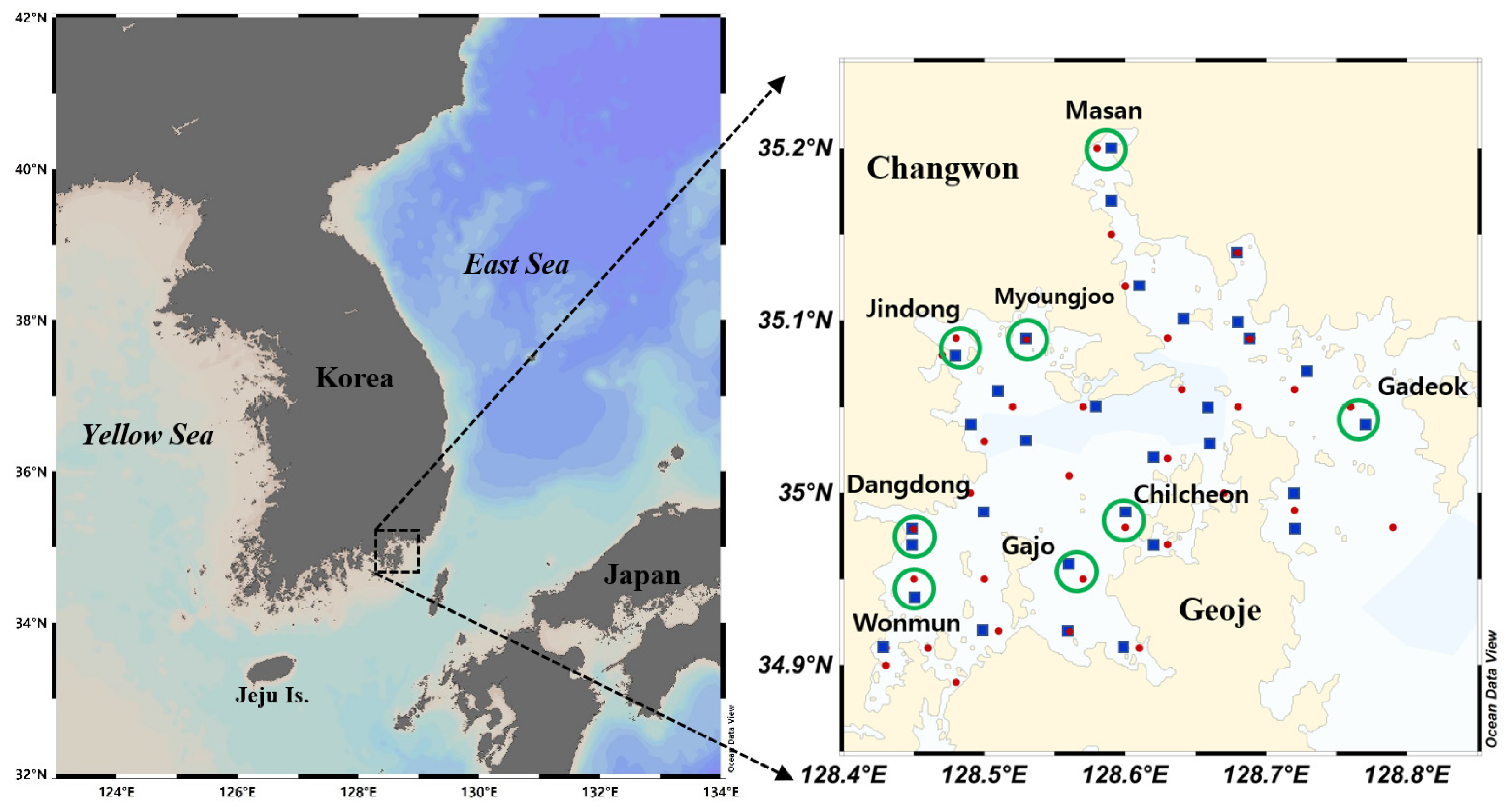
2.1. Study Area

Jinhae Bay is a semi-enclosed bay surrounded by Changwon City and Geoje City, with seven sub-bays (Masan Bay, Jindong Bay, Danghang Bay, Dangdong Bay, Wonmun Bay, Gohyeon Bay, and Haengam Bay; Figure 1). Its shoreline spans 436.7 km, with a mean and maximum water depth of 20 m and 45 m, respectively. The volume of seawater exchange through Gadeok Channel during the spring tide is 471–507 × 10⁶ m³, accounting for 84–90% of the total seawater exchange in Jinhae Bay [23]. The farming area of Jinhae Bay has a dense, concentrated distribution on the west side of Jinhae Bay, encompassing Jindong Bay and Dangdong–Wonmun Bay. The main product of the aquaculture industry in the region is shellfish, including oysters, mussels, and blood cockles. According to national fishery statistics, 80–90% of oysters and 95% of mussels are produced on the eastern coast of the South Sea of Korea, which includes Jinhae Bay.

Jinhae Bay is well known as a habitat and spawning and nursing ground for major fishery resources on the southern coast of Korea. However, since the 1970s, the discharge of domestic sewage, industrial effluent, and other pollutants into Jinhae Bay has continually increased owing to industrialization and intensive aquaculture, exceeding the self-purification capacity of the bay, which has led to a rapid spread of eutrophication across the region. Jinhae Bay was the first region in South Korea reported to experience harmful algal blooms (HABs) due to eutrophication, and in 1967, mass mortality events on oyster farms caused by hypoxia from large-scale HABs were reported [24]. Therefore, to improve the water quality in Jinhae Bay, several projects have been implemented, including the dredging of the bottom sediment and the construction of wastewater treatment plants, which have improved the water quality by reducing the chemical oxygen demand (COD) and dissolved inorganic phosphate (DIP) concentrations [25]. Long-term (2000 and 2012) analysis of the nutrient concentrations also showed a marked decrease, demonstrating an improvement in the water quality of the region [26].

Despite these management and conservation efforts, hypoxia continues to occur annually during summer across Jinhae Bay [6,27]. From September to October 2008, severe hypoxia resulted in a loss of KRW 54.9 million across 68 fish farms in Masan and Geoje waters, and from August to October 2012, the damage amounted to KRW 2.213 billion across 172 cases and included losses at oyster and sea squirt farms.

2.2. Field Survey, Water Quality Analysis, and Meteorological Data

The field survey of this study was conducted from 2011 to 2016 using the research vessel Tamgu 7 of the National Institute of Fisheries Science, and it was based on 31–34 stations in Jinhae Bay (Figure 1). Regular surveys were conducted in even-numbered months, and additional surveys (once or twice a month) were conducted from May to September, which is the hypoxia development period. To examine the status of the hypoxia development by sea area in Jinhae Bay, eight stations were selected as representative stations: Gadeok Channel as a control station, and major sub-bays, namely, Masan Bay, Myoungjoo Bay, Jindong Bay, Dangdong–Wonmun Bay 1, Dangdong–Wonmun Bay 2, Gajo Island, and Chilcheon Island. The survey stations were the same from 2011 to 2012, and from 2013 to 2016, the survey was conducted by moving the stations to locations closer to the surrounding fish farms.

Vertical profiles of the temperature and salinity of the seawater were monitored using a CTD profiler (19plusV2, Sea-Bird Electronics, Bellevue, WA, USA), and the pH and DO concentrations were measured using a multi-parameter water quality sonde (6600-v2, YSI, Yellow Springs, OH, USA). The pH sensor underwent periodic inspection and was calibrated using YSI’s pH 4.00, pH 7.00, and pH 10.00 standard buffer solutions before use. For the DO, part of the seawater sample (surface/bottom water) was collected and titrated based on the Winkler method using a titrator (Dosimat 876 system, Metrohm, Herisau, Switzerland) with a precision of ±3% to compare and determine the deviation in the YSI values.

Seawater samples were collected from the surface (1–2 m below the sea surface) and bottom (2–3 m above the sea floor) using a Niskin sampler. For the nutrients and chlorophyll a (Chl-a), surface and bottom waters were filtered on-site through a 0.45 μm membrane filter, and the filtered seawater and filter paper necessary for analysis were stored frozen. The frozen samples were transferred to a laboratory and analyzed according to the MOF [28]. Nutrients were analyzed using a continuous-flow auto-analyzer and the analysis results were verified against relevant reference materials (reference materials for nutrients in seawater, KANSO TECHNOS CO. LTD., Osaka, Japan). Duplicate analyses suggest that the measurement precisions for the nitrate, ammonium, phosphate, and silicate were ±3%, ±4%, ±2%, and ±3%, respectively.

In addition, meteorological data, including the air temperature, precipitation, wind speed, and sunshine duration in Changwon, Gyeongsangnam-do, which represented the study area, were used as daily/weekly/monthly averages and totals as required for the period from 2011 to 2016 (www.kma.go.kr (accessed on 1 July 2022)).

The Pearson correlation was carried out to study the relationships between the water/meteorological data and hypoxia indices, and the Levene’s test was used to test for the homogeneity of the data. The statistical analyses were performed using the SPSS for Windows software package, ver. 12.0 K (IBM Corp., Armonk, NY, USA), and p < 0.05 was considered indicative of statistical significance.

2.3. Hypoxic Indices

To analyze the patterns of hypoxia development in Jinhae Bay, several hypoxia-related indices were selected, such as the hypoxia area, minimum DO concentration, hypoxia thickness, and hypoxia duration. In this study, the threshold concentration of hypoxia was set as a seawater DO concentration of ≤3 mg/L, which is the limit concentration that threatens marine organisms [1,2] and is consistent with the database of the National Fisheries Research and Development Institute [29].

Regarding the areal extent of the hypoxia development in Jinhae Bay, an area with a DO concentration ≤ 3 mg/L in the bottom water, spanning from 34.85°–35.25° latitude to 128.4°–128.7° longitude, was used. At each survey station, the minimum DO concentration, hypoxia thickness, and hypoxia duration were used as the evaluation indices. The lowest DO concentration measured at each station was used as the minimum concentration, and the product of the duration in weeks and the depth of water with a DO concentration ≤ 3 mg/L was used as the hypoxia thickness. The time from the initiation of the hypoxia to its termination in the unit of weeks was used as the duration of the hypoxia. The water stability index was calculated by dividing the density difference between the surface and bottom waters by the water depth (ρ_{SW (B-S)}/H) [30].

3. Results

3.1. Environmental Characteristics

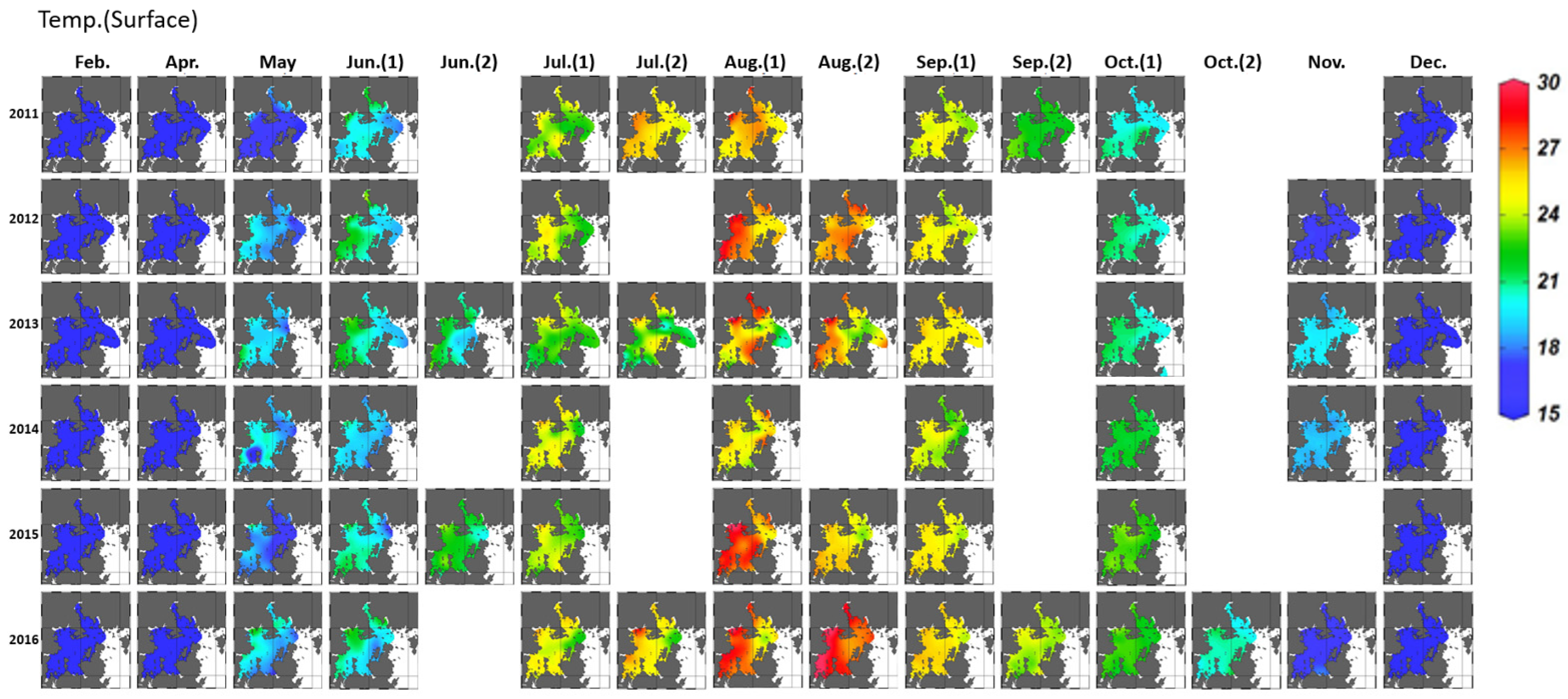
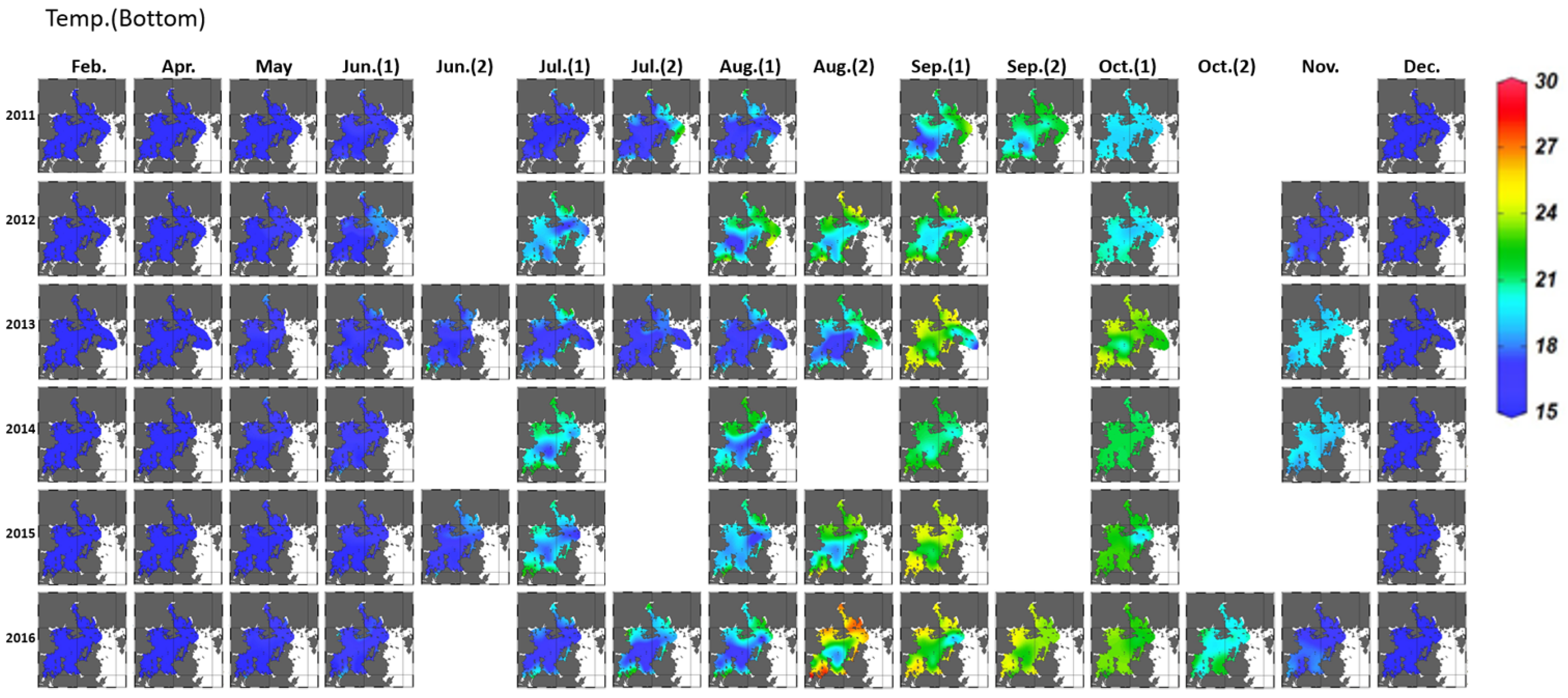
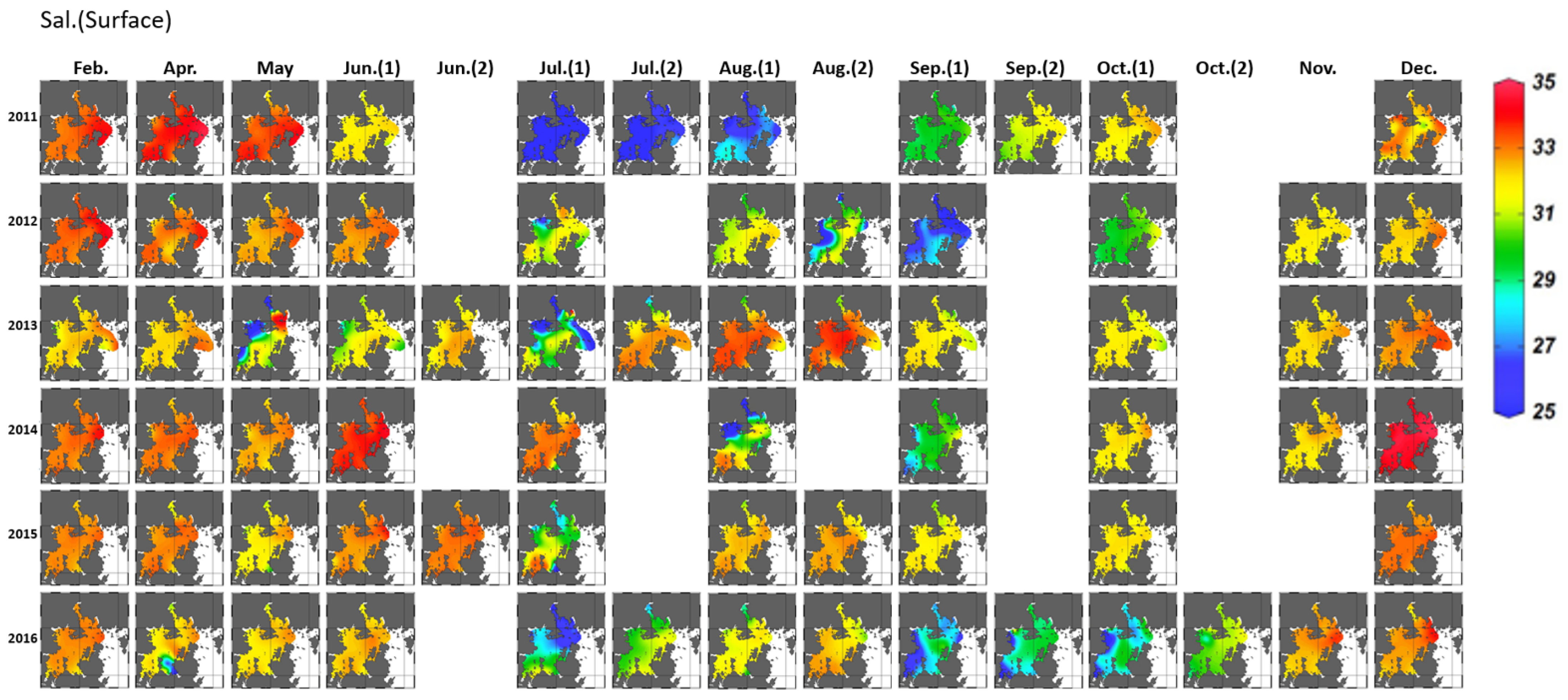
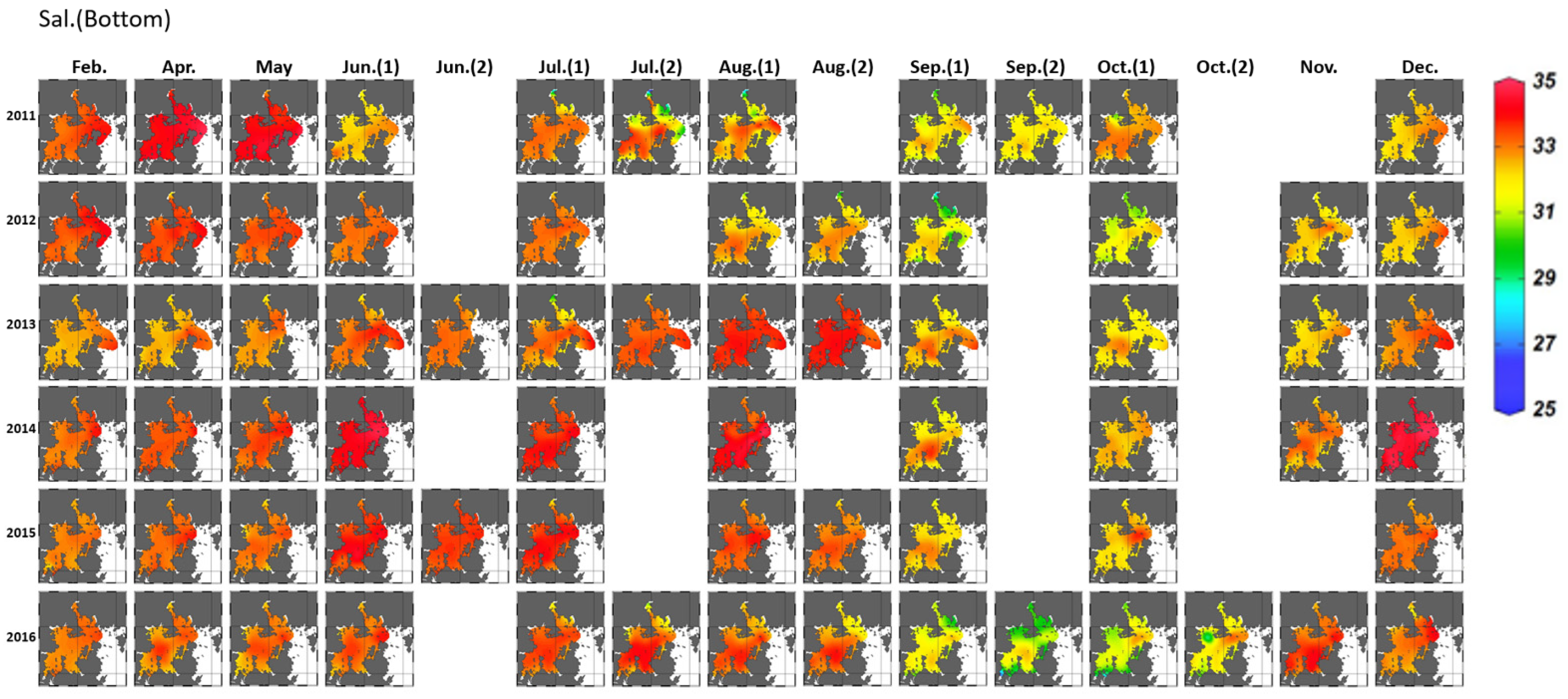
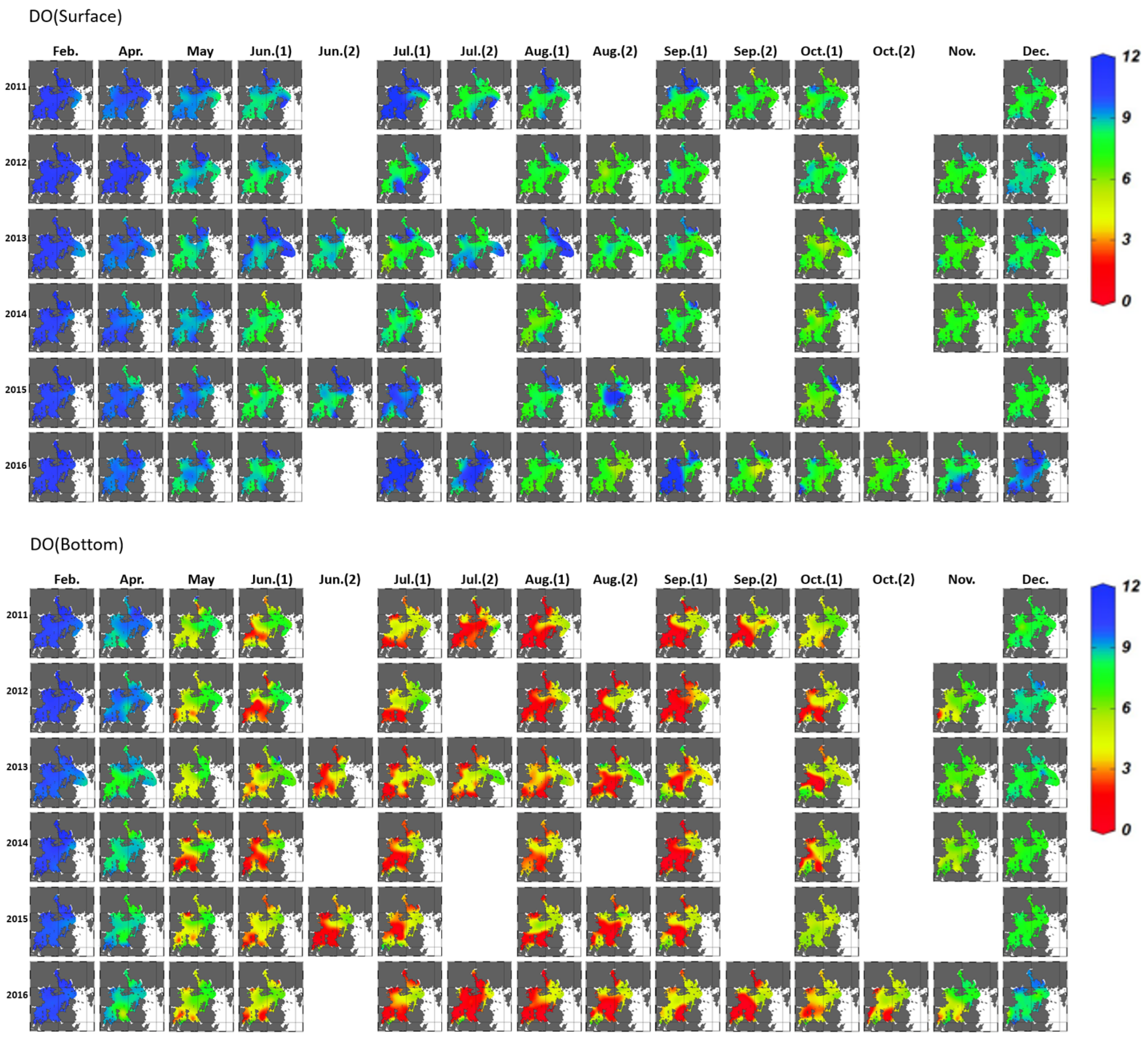
3.1.1. Variation in Seawater Quality

The measurements of the water temperature, salinity, and DO concentration during the entire survey period are presented in Figure 2, Figure 3 and Figure 4. During the survey period, the temperature showed a seasonal pattern and interannual variation. Distinct seasonal trends were observed for the surface-water temperature, which was low in winter (lowest: 4.6 °C in February 2012) and high in summer (highest: 28.5 °C in August 2016) (Figure 2). The annual average of the water temperature, based on 6 even months, ranged from 15.3 to 17.0 °C, with the highest in 2015 and the lowest in 2012. Especially in August, the average water temperature ranged from 25.1 to 28.5 °C in the surface water and from 17.5 to 24.8 °C in the bottom water, with relatively high temperatures in 2012, 2015, and 2016. In August 2016, the average surface-water temperature was 28.5 °C (26.6–31.0 °C), which was higher than that (25.1–27.5 °C) in the other years. In 2013 and 2016, the average temperature remained higher than 23 °C, even in October. The bottom-water temperature exhibited the same seasonal patterns as those of the surface-water temperature. Especially in the summer season, the bottom-water temperature was generally higher in 2016 and lower in 2011 than that in the other years.

During the study period, the average salinity ranged from 16.3 to 34.4 and from 31.4 to 34.5 for the surface and bottom waters, respectively (Figure 3). The surface-water salinity in 2011 was low (8.33–28.60) in July and August; however, there was no significant difference in the bottom-water salinity, even in July. In 2016, the surface- and bottom-water salinities were relatively low at 11.88–31.46 and 27.75–33.34 in September and October, respectively. In 2012, the surface-water salinity was relatively higher (from 29.95 to 33.88) than that in the other years, and the bottom-water salinity was high for most of the study area.

The average DO concentration ranged from 6.6 to 12.6 mg/L and from 2.0 to 10.4 mg/L for the surface and bottom waters, respectively, during the survey period. The surface DO concentration did not vary significantly, except for at a few stations in summer, with a monthly average ranging from 6.55 to 12.75 mg/L. The DO in the bottom water was generally high in winter and low in summer (Figure 4). The DO in the bottom water from June to September of each year was <5 mg/L on average, with relatively low values in 2012, 2014, and 2016. In 2014, the monthly average DO from June to September ranged from 2.0 to 3.4 mg/L, with the lowest in September. Also in 2016, the lowest average DO was measured in late July–early August, with a value of 2.1 mg/L.

The average pH values ranged from 7.77 to 8.39 and from 7.58 to 8.14 in the surface and bottom waters, respectively, from 2011 to 2016. High pH values were observed in the surface water every summer, with the highest in July of 2011. In contrast to the surface water, the pH value in the bottom water gradually decreased in summer, reaching values of <7.7 on average, with the lowest in August 2014. The spatial distribution of and seasonal variation in the pH in the bottom water were similar to those of the DO, suggesting the relation between hypoxia and acidification in coastal waters.

The average nitrate concentrations ranged from 0.2 to 32.8 μmol/L and from 0.3 to 8.8 μmol/L in the surface and bottom waters, respectively. The average nitrate concentration in the surface water was 32.8 μmol/L in July 2011, and the nitrate concentration was high in almost all the waters in the study area. In October 2016, high concentrations were also observed in certain areas, including Gadeok Channel and the inner part of the sub-bays. High concentrations were measured in the bottom water in the month when the concentration in the surface water was high and the following month. In addition, the nitrate concentrations were relatively high both in the surface and bottom waters in December of every year except 2016; in this case, the concentration in Gadeok Channel was the highest, and the values decreased toward the inner side of Jinhae Bay (Supple. 1). Measurements of the average ammonium ranged from 0.3 to 7.3 μmol/L and from 0.4 to 11.6 μmol/L in the surface and bottom waters, respectively. In contrast to the nitrate concentration, the distribution of the ammonia concentration in the surface water did not change significantly, and high values were measured in certain areas, including Masan Bay and Jindong Bay. The ammonium concentration in the bottom water was high from July to September for every year; however, in 2013, the concentration trend changed such that the measurements were low from August to September and high in October (Supple. 2). The phosphate concentrations ranged from 0.05 to 0.99 μmol/L and from 0.11 to 1.56 μmol/L in the surface and bottom waters, respectively. The surface-water phosphate concentration was the highest in December except in 2016, and very low (average < 0.2 μmol/L) in spring and summer, except for Masan Bay. In contrast to the surface water, the phosphate concentration in the bottom water gradually increased in summer, reaching values of >1 μmol/L on average (Supple. 3). The silicate concentrations ranged from 1.5 to 58.3 μmol/L and from 1.6 to 52.6 μmol/L in the surface and bottom waters, respectively. The surface water silicate concentration was the highest in July 2011 and August 2014. In the bottom water, the silicate concentration was relatively low (average < 10.0 μmol/L) in winter and high (average > 30.0 μmol/L) in summer. The spatial distribution of and seasonal variation in the silicate were similar to those of the nitrate.

The average Chl-a concentration ranged from 0.1 to 38.3 μg/L and from 0.1 to 10.0 μg/L in the surface and bottom waters, respectively, from 2011 to 2016. High concentrations were observed in the surface water every summer, and the average Chl-a concentration in July of 2011 was 38.3 μg/L (a range of 6.4–140 μg/L) and was high at all stations except for the area on the eastern coast of Geoje Island. Comparing the study areas, Masan Bay had higher concentrations than the other areas throughout the year. In June of 2012 and 2013, high concentrations of 835 μg/L and 142 μg/L were measured in the surface water, respectively. In addition, the average concentrations in February 2011 and December 2016 were 9.7 μg/L and 19.0 μg/L in the surface waters, respectively, presenting high values despite it being the winter season (Supple. 4).

For 2011–2016, the correlation between the water quality parameters of the surface and bottom waters was analyzed (

Table 1. Correlation coefficients between the water quality parameters in Jinhae Bay from 2011 to 2016 (surface water).

	Temperature	Salinity	pH	Dissolved Oxygen	Ammonia	Nitrate	Nitrite	Phosphate	Silicate	Chlorophyll a
Temperature	1	−0.327 *	0.342 *	−0.305 *	0.037	0.109	0.116	0.168	0.131	0.220
Salinity		1	−0.468 **	−0.231	−0.332 *	−0.796 **	−0.466 **	−0.141	−0.617 **	−0.563 **
pH			1	0.528 **	−0.253	0.110	0.034	−0.375 **	−0.021	0.306 *
Dissolved Oxygen				1	−0.413 **	0.161	−0.166	−0.576 **	−0.035	0.388 **
Ammonia					1	0.475 **	0.325 *	0.853 **	0.550 **	−0.174
Nitrate						1	0.496 **	0.349 *	0.861 **	0.406 **
Nitrite							1	0.389 **	0.506 **	0.204
Phosphate								1	0.500 **	−0.155
Silicate									1	0.415 **
Chlorophyll a										1

** p < 0.01; * p < 0.05.

and

Table 2. Correlation coefficients between the water quality parameters in Jinhae Bay from 2011 to 2016 (bottom water).

	Temperature	Salinity	pH	Dissolved Oxygen	Ammonia	Nitrate	Nitrite	Phosphate	Silicate	Chlorophyll a
Temperature	1	−0.512 **	−0.266	−0.739 **	0.514 **	0.195	0.402 **	0.596 **	0.321 *	0.022
Salinity		1	0.105	0.300 *	−0.436 **	−0.457 **	−0.453 **	−0.389 **	−0.052	0.033
pH			1	0.616 **	−0.266	−0.456 **	−0.106	−0.429 **	−0.429 **	−0.500 **
Dissolved Oxygen				1	−0.470 **	−0.346 *	−0.285 *	−0.625 **	−0.660 **	−0.184
Ammonia					1	0.414 **	0.302 *	0.844 **	0.554 **	−0.047
Nitrate						1	0.475 **	0.491 **	0.428 **	0.087
Nitrite							1	0.379 **	0.322 *	−0.082
Phosphate								1	0.639 **	−0.078
Silicate									1	−0.028
Chlorophyll a										1

** p < 0.01; * p < 0.05.

). The surface-water DO concentration was negatively correlated with dissolved inorganic nutrients such as ammonium (r = −0.41, p < 0.01) and phosphate (r = −0.58, p < 0.01) and positively correlated with Chl-a (r = 0.39, p < 0.01). The bottom-water DO concentration was strongly correlated with the temperature (r = −0.74, p < 0.01) and correlated with the pH (r = 0.62, p < 0.01) and nutrient concentration (r = −0.66–−0.29, p < 0.01 or 0.05). The dissolved inorganic nutrients were positively correlated with each other in both the surface (r = 0.33–0.86, p < 0.01 or 0.05) and bottom (r = 0.30–0.84, p < 0.01 or 0.05) waters. Thus, there was a significant correlation between the hypoxia development in the bottom water and increases in the bottom-water temperature and nutrient concentration, as well as decreases in the pH. In addition, because the concentrations of different dissolved inorganic nutrients were correlated with each other in the surface and bottom waters, it can be inferred that changes in the distribution of these nutrients and their inputs and outputs are controlled by similar factors and sources. This result is consistent with that of Kwon et al. [26], who analyzed long-term variations in the water quality of Jinhae Bay and inferred that freshwater inputs or nutrient release from bottom sediments affected the changes in the water quality. In particular, in the case of the bottom water, the observed trend was consistent with previous studies that found that the active degradation of organic matter in bottom water contributed to increased nutrient loading [26,31].

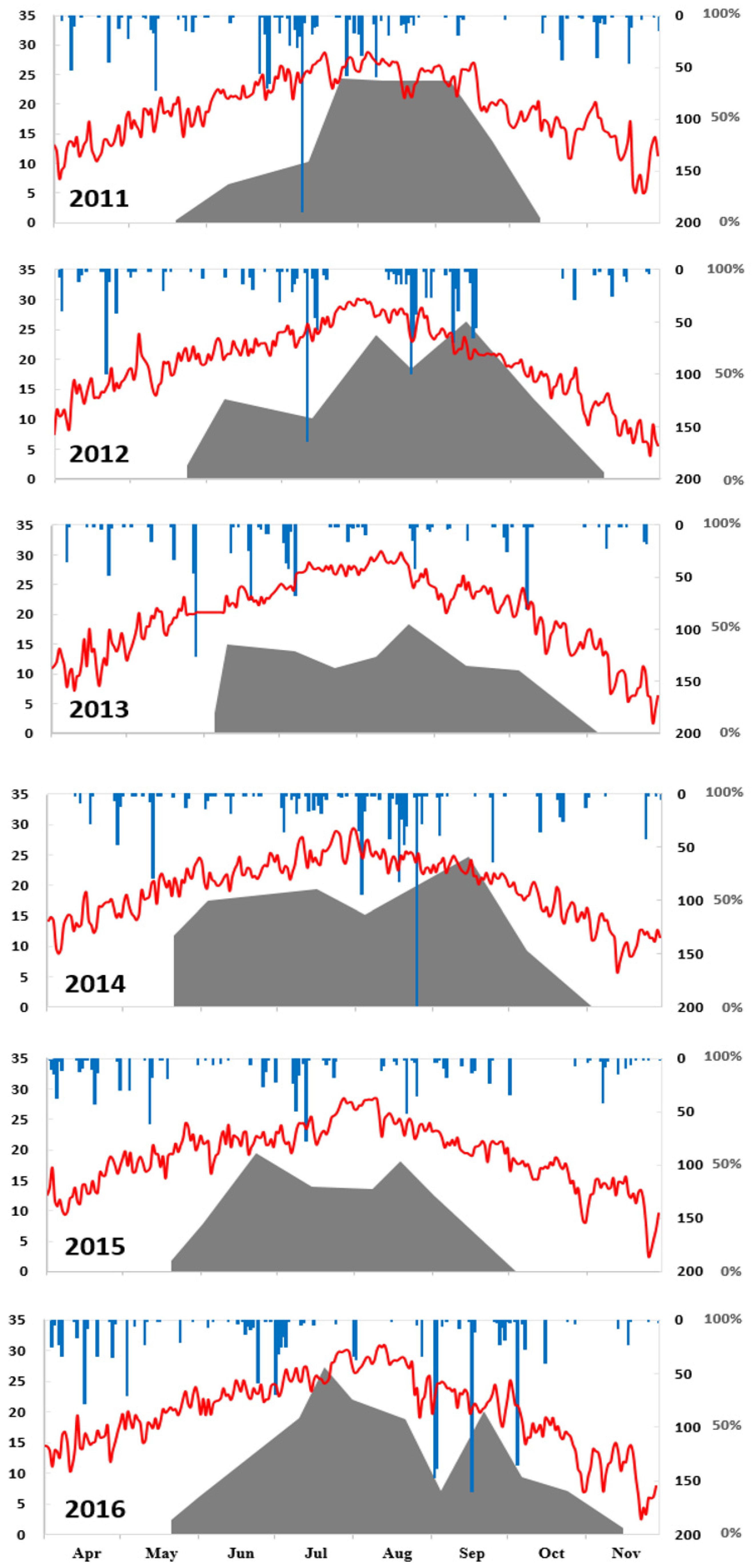
3.1.2. Meteorological Data

Regarding the meteorological data from April to October from 2011 to 2016, monthly average values were used for the air temperature and wind speed and monthly sum values were used for the precipitation, and the values were compared with averages obtained from 20-year historical data.

The air temperatures in 2015 were generally lower than those of other years, and from June to October in particular, the temperatures were 0.5–2.0 °C lower than that of the 20-year average. In 2013, the temperatures were higher than those of other years, and in July and August, the temperatures were 1.8 °C and 1.5 °C higher than the average, respectively (

Table 3. Monthly average air temperature, total rainfall, and wind speed measured at Changwon Station, Korea, from 2011 to 2016, with 20-year averages.

		January	February	March	April	May	June	July	August	September	October	November	December
Air Temperature (°C)	Average (’90–’10)	2.9	4.8	8.7	14.0	18.3	21.7	25.2	26.4	22.9	17.6	10.9	5.1
	2011	−1.1	5	7.1	12.9	17.9	21.9	25.6	25.7	23	16.5	13.1	3.8
	2012	2.2	2.1	7.9	14	19.1	21.8	26.0	27.5	21.9	16.8	9.4	1.7
	2013	1.3	3.6	9.6	12.5	18.7	22.4	27.0	28.0	23.3	18.3	10	4.7
	2014	4.0	5.4	9.6	14.5	19.4	22	25.2	24.6	22.3	17.2	11.6	2.9
	2015	3.6	4.6	8.9	13.9	19.3	21.2	24.1	25.4	20.9	16.4	11.8	5.5
	2016	0.6	4.1	8.9	14.7	19.4	22.5	26.3	27.3	22.2	17.4	9.8	5.4
Rainfall (mm, monthly sum)	Average (’90–’10)	31.7	48.1	77.0	129.8	161.6	208.4	328.5	313.0	164.8	54.9	44.7	23.3
	2011	0.0	74.7	26.9	149.6	147	238	414.1	198.5	27.9	91.5	141.2	4.6
	2012	5.2	11.0	101.4	217.4	39.9	78.9	334.6	329.6	269	37.0	56.2	79.2
	2013	13.7	71.2	84.9	90.5	222.4	148.5	190.1	82.3	58.5	83.2	59.6	5.1
	2014	5.7	20.0	152.5	102.9	106.5	45.1	149.2	665.9	109.8	101.0	51.5	15.7
	2015	33.4	31.0	69.5	196.3	134.0	77.0	197.5	116.7	88.9	40.2	85.2	41.0
	2016	40.5	73.2	81.6	263.0	123.7	108.8	181.8	110.0	522.7	215.8	35.1	136.8
Wind Speed (m/s)	Average (’90–’10)	2.2	2.2	2.3	2.3	2.2	2.1	2.2	2.0	1.9	1.8	1.9	2.0
	2011	2.6	1.7	2.2	2.4	2.1	2.2	2.2	1.8	1.8	1.6	1.5	2.1
	2012	2.2	2.1	2.1	2.4	1.9	1.9	1.9	2.2	1.7	1.5	1.9	2.2
	2013	2.0	2.1	2.3	2.3	2.0	1.7	2.3	1.7	1.6	1.7	1.7	1.9
	2014	1.8	2.1	1.9	1.8	2.0	1.6	1.4	2.0	1.5	1.7	1.5	1.9
	2015	1.9	1.9	2.1	2.0	2.0	1.8	1.8	1.4	1.5	1.4	1.3	1.6
	2016	1.9	1.9	1.7	1.7	1.7	1.5	1.4	1.4	1.1	1.4	1.6	1.8

).

The wind speed from 2011 to 2016 was measured at monthly averages of 1.1–2.4 m/s. In late August and mid-September 2012, the daily average wind speeds were very high, at 8.2 m/s and 5.0 m/s, respectively, due to the influence of the typhoons Bolaven and Sanba.

Compared to other meteorological factors, the precipitation showed larger monthly variations each year. The total monthly rainfall in 2014 was 665.9 mm in August (the 20-year maximum was 328.5 mm), which was the highest value recorded for the entire study period. The autumn rainfall values in 2016 were 522.7 mm in September and 215.8 mm in October, which were markedly higher than the 20-year averages (Table 3).

3.2. Characteristics of Hypoxia Development

3.2.1. Horizontal Distribution and Duration of Hypoxia Development

The characteristics of the hypoxic water in Jinhae Bay were examined from May to November of 2011–2016 based on the DO concentration of the bottom water (Figure 5 and

Table 4. Information regarding the development of hypoxia in Jinhae Bay from 2011 to 2016.

	2011	2012	2013	2014	2015	2016
Occurrence	early-Jun	end-May	early-Jun	end-May	end-May	end-May
Average in Jun–Oct (km2)	164	205	140	201	142	176
Maximum area (km2)	284	308	213	289	227	316
Period of maximum area	end-Jul	mid-Sep	end-Aug	mid-Sep	end-Jun	end-Jul
Duration (weeks)	15	22	18	20	20	26

). Hypoxia in Jinhae Bay occurred from May to June during most of the survey years, and, in terms of the spatial distribution, hypoxia initiation was observed in the sub-bays, including Wonmun Bay, Jindong Bay, the east of Gajo Island, and Masan Bay. The hypoxia that developed in the sub-bays extended to the center of Jinhae Bay from July to September, showing the maximum areal extent of the hypoxia development. From September to November, as the area of the hypoxia development decreased, the hypoxic zone remained in the sub-bays (including Wonmun Bay and Jindong Bay), which are regions of hypoxia initiation, and, over time, the hypoxia disappeared.

The maximum hypoxic area of each year increased in the following order: 2013 (August), 2015 (June), 2011 (July), 2014 (September), 2012 (September), and 2016 (July) (Table 4). In 2012 and 2016, the maximum area exceeded 300 km² (> 75% of the total area of Jinhae Bay), and in 2013 and 2015, the hypoxia development was relatively weak (and narrow) at 213 km² (52%) and 227 km² (56%), respectively. The duration of hypoxia was also the longest from May to November in 2012 and 2016, the years when the development area was the largest, and it was short during five months of 2011 and 2013 (from June to October) and 2015 (from May to September), the years when the development area was small. During the seasonal cycles of hypoxia (initiation–persistence(re-expanding)–termination), two or three peaks repeated during the persistence phase, with expansions and contractions of the hypoxic area identified in most years, and only one peak of hypoxia development was observed from initiation to termination in 2011.

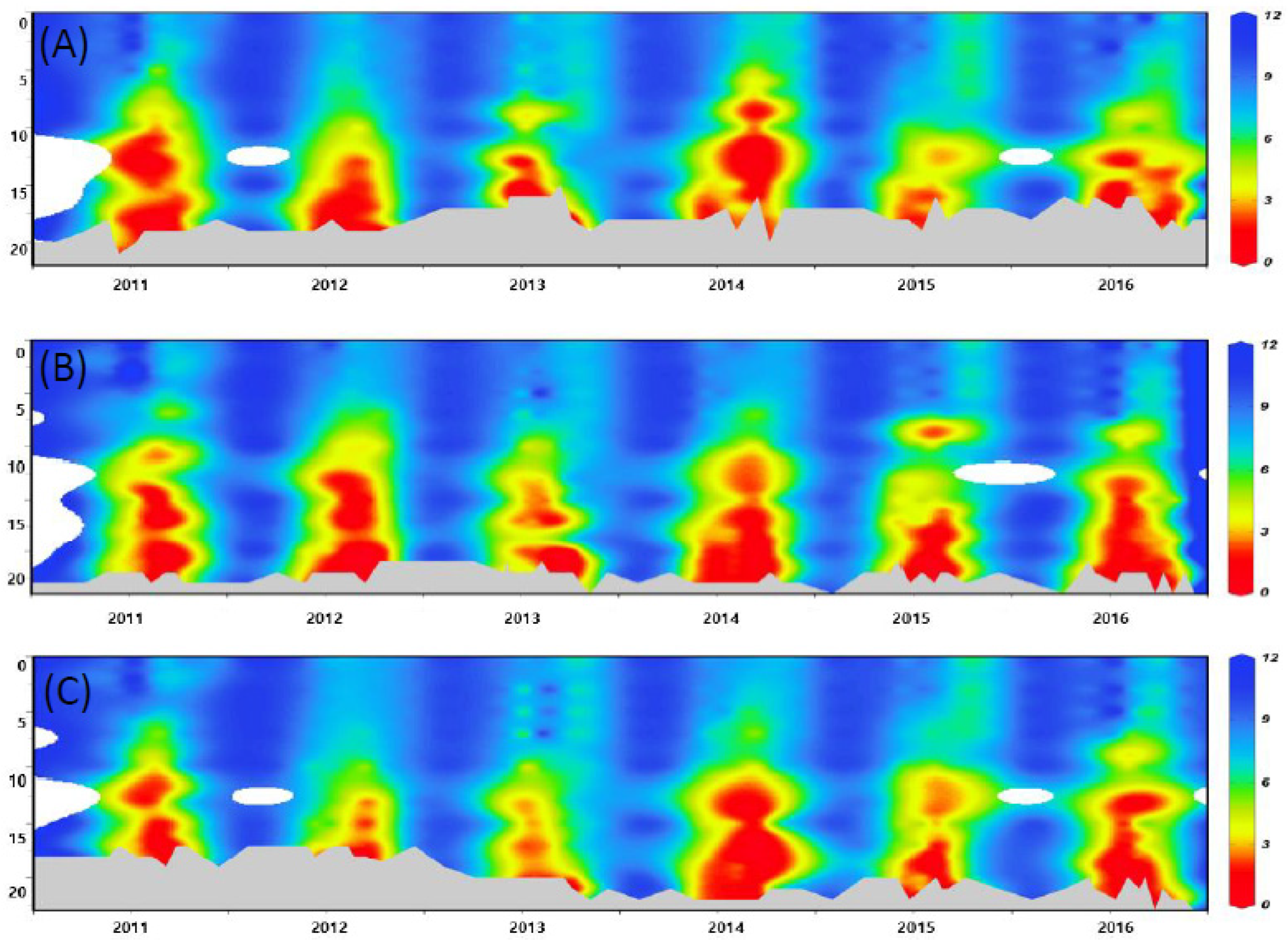
3.2.2. Vertical Distribution and Strength of Hypoxia

To investigate the patterns of the hypoxia development in the water columns, the vertical distributions of the DO concentrations in the representative stations are shown as time series from 2011 to 2016 (Figure 6). The hypoxia development in Wonmun Bay had the shortest durations in 2013 and 2015, and the intensity was from the bottom to a depth of 10 m. This increased to a depth of 7 m in 2014, and the hypoxia development persisted for longer in 2016, showing a pattern of initiating, expanding, weakening, and then re-expanding. The hypoxia development in the eastern part of Gajo Island had the longest durations in 2012, 2014, and 2016, and the zone of hypoxic water was also large. The hypoxia around Chilcheon Island showed strong development in 2014 and 2016. At all three stations, hypoxia developed for the longest duration and over the vertically broad areas of the water column in 2014.

The minimum DO concentration, thickness of the hypoxic water column, and duration of hypoxia development were calculated for each representative station from 2011 to 2016 (

Table 5. Hypoxia indices at control station and major sub-bay stations from 2011 to 2016.

	Minimum Concentration (mg/L)						Thickness						Duration (Weeks)
Year	2011	2012	2013	2014	2015	2016	2011	2012	2013	2014	2015	2016	2011	2012	2013	2014	2015	2016
Average	0.47	0.50	0.52	0.35	0.67	0.43	64.9	71.9	45.0	111.2	54.7	96.1	10.5	19.8	12.9	18.7	11.4	17.1
Gadeok	5.29	5.01	3.95	5.06	4.76	4.04
Masan	1.40	1.40	1.25	0.7	0.9	0.33	7	30	36	41	23	66	4	14	17	9	10	10
Myoungjoo	0.38	0.38	0.43	0.34	0.28	0.93	22	24	20	88	51	56	4	9	7	27	15	13
Jindong	0.28	0.33	0.39	0.32	1.12	0.48	81	60	17	64	33	60	11	18	2	18	10	21
Dangdong–Wonmun 1	0.28	0.50	0.42	0.32	1.58	0.44	91	124	42	119	48	93	15	29	19	20	10	15
Dangdong–Wonmun 2	0.24	0.23	0.51	0.25	0.27	0.33	85	87	47	150	59	122	15	22	11	20	11	15
Gajo	0.26	0.17	0.28	0.26	0.3	0.29	99	132	84	170	98	153	15	29	19	20	15	21
Chilcheon	0.43	0.49	0.39	0.27	0.27	0.22	68	46	70	147	71	124	8	18	13	17	10	24

). The minimum concentration, thickness (total), and duration (in weeks) ranged from 0.17 to 1.58 mg/L, from 7.0 to 170, and from 4 to 29 weeks, respectively. Regarding the average values of the representative stations by year, the minimum DO concentration was the lowest (0.35 mg/L) in 2014, and the hypoxic water column thickness was the highest in 2014 at 111.2. The duration was the longest (19.8 weeks) in 2012. The minimum DO concentrations in 2013 and 2015 were relatively high (>0.5), and the thickness and duration of the hypoxia were relatively low and short, respectively. During the study periods, hypoxic water masses were not observed in Gadeok Channel, which was the control area with an annual DO concentration of ≥3 mg/L.

4. Discussion

4.1. Analysis of Factors Influencing Hypoxia

Correlations between the hypoxia indices (minimum DO concentration, hypoxic-layer thickness, and hypoxic area) and water quality parameters were examined (

Table 6. Correlation coefficients between hypoxia indices and water/weather parameters at stations of major sub-bays during hypoxic period (April–October).

		Hypoxic Area	Minimum Concentration	Thickness	Stability
Surface Water	Temperature	0.670 **	−0.873 **	0.208	0.349 **
	Salinity	−0.185	0.352 **	−0.255	−0.878 **
	DO	−0.131	0.282 *	0.080	0.294 *
	Ammonia	−0.071	−0.021	0.297	0.298 *
	Nitrate	−0.055	−0.088	0.099	0.812 **
	DIP	−0.081	−0.136	0.082	0.110
	DSi	−0.119	−0.221	0.155	0.684 **
Bottom Water	Temperature	0.328 *	− 0.725 **	0.077	0.056
	Salinity	−0.111	0.298 *	−0.065	−0.045
	DO	−0.805 **	−0.998 **	−0.614 **	−0.333 *
	Ammonia	0.211	−0.480 **	0.499 **	0.313 *
	Nitrate	0.131	−0.355 *	0.384 *	0.669 **
	DIP	0.353 *	−0.634 **	0.406 *	0.347 *
	DSi	0.179	−0.675 **	0.484 **	0.393 **
Weather Parameter	Temperature	0.638 **	−0.815 **	0.185	0.440 **
	Rainfall (4 weeks)	0.457 **	−0.338 *	0.471 **	0.191
	Wind speed	−0.010	0.160	−0.131	0.407 **
	Daylight hours	−0.268	0.236	−0.065	−0.409 **

** p < 0.01; * p < 0.05.

). The surface-water temperature was strongly correlated with the hypoxic area (r = 0.67, p < 0.01) and minimum DO concentration (r = −0.87, p < 0.01), and the surface salinity was correlated with the minimum DO concentration (r = 0.35, p < 0.01). In addition, the bottom-water temperature was correlated with the hypoxic area (r = 0.33, p < 0.05) and minimum DO concentration (r = −0.73, p < 0.01). These results indicate that a water mass with a higher temperature and lower salinity has a greater likelihood of developing larger-scale and stronger hypoxia due to the strengthening of the stratification in the water column. The largest hypoxic area (approximately 316 km²) developed in July–August 2016, when the surface-water temperature was 24.7 °C, representing the hottest July of the study period. The hypoxic area was broader when the average surface salinity was below approximately 30 from 2 weeks to 1 month, such as in May–June in 2013, July–August in 2011, and September–October in 2016. A hypoxic area of more than 230 km² was maintained from late July to early September of 2011, when the average surface salinity was in the range of 16.3–29.6. In 2013 and 2016, the hypoxic area expanded by 3–4 times during short periods of 1–2 weeks (from 39 to 174 km² within 1 week in June 2013 and from 82 to 233 km² within 2 weeks in September 2016), corresponding with the lowest salinities observed in May and June (29.0–31.2) as well as in September and October (27.4–28.1).

Among the hypoxia indices, the minimum DO concentration showed significant correlations with the water temperature (r = −0.73, p < 0.01), concentrations of nutrients (r = −0.68–−0.36, p < 0.01 or 0.05), and DO (r = −0.99, p < 0.01), especially in the bottom water. After hypoxia had developed and the supply of DO from the surface was interrupted, oxygen consumption via biogeochemical processes in the water column accelerated, intensifying the oxygen deficiency in the water column. DO consumption occurs in the water column due to several processes, including the decomposition of organic matter, complex nitrogen oxidation–reduction reactions, material diffusion through the water–sediment interface, and biological respiration. When organic matter degradation and consecutive chemical redox processes occur, nutrients released through these processes increase in concentration within the water column; most of these processes become faster at higher temperatures. Thus, among the hypoxia indices, the minimum DO concentration showed a significant correlation with the bottom temperature, influenced by the reaction time of the organic matter decomposition and the nutrients released as byproducts. Therefore, the minimum DO concentration is an index representing the intensity of the hypoxia in the water column, and a related index, the thickness of the hypoxic layer, is also associated with the nutrients in the bottom water.

As the DO decreases at the sediment–water interface and the environment gradually becomes anaerobic, ammonium is generated preferably over nitrate and nitrite; therefore, a stronger correlation was found for hypoxia indices with ammonium than for those with nitrate or nitrite. The average (range) concentration of ammonium at the representative stations was 2.5 μM (0.5–4.7 μM) from April to June and increased to 6.4 μM (3.1–16.5 μM) from July to September (hypoxia season). These results coincide with the process of nitrogen cycling described by Huang and An [32], who reported the following results regarding benthic nitrogen cycling under both normoxic and hypoxic conditions in Jinhae Bay: among the nitrate reduction processes, dissimilatory nitrate reduction to ammonium is dominant in Jinhae Bay due to the sulfidic and richly organic sediments; in hypoxic environments, denitrification increases, and the sediment is a continuously available source of ammonium under both normoxic and hypoxic conditions. Based on measurements of the oxygen demand in the water column (WOD) driven by microbial activity in Jinhae Bay, a constant WOD was maintained, even in hypoxic environments [33], which is consistent with weak hypoxia that intermittently supplies oxygen to shallow water depths [32]. Ammonium, but not other nitrogen forms, is produced continuously in hypoxic environments and thus shows stronger relationships with the indices of hypoxia. Park et al. [33] also noted that the WOD increased with the increasing water temperature and found significant positive correlations between these factors in Jinhae Bay. These findings are consistent with the strong positive correlations of the bottom-water temperature with the hypoxic area and minimum DO concentration presented in Table 6.

In addition, the relationships between the water quality parameters and the water stability index, which is closely related to hypoxia development, were examined [8,9]. The water stability showed strong correlations with the salinity, nitrate, and silicate concentrations in the surface water (r = −0.88, 0.81, and 0.68, p < 0.01), as well as with the nitrate and silicate in the bottom water (r = 0.67 and 0.39, p < 0.01). These results indicate that the stability was mainly controlled by the delivery of water masses from coastal areas that are less saline and more eutrophic, generally via massive river discharges after heavy rain. Therefore, the inflow of freshwater may be a strong driver of hypoxia that acts by intensifying both the stratification and eutrophication.

When the total monthly rainfall was high in July 2011 (414 mm) and August 2014 (666 mm), the surface-salinity average among all the stations reached minima of 16.3 and 28.3 psu, respectively. The survey in July 2011 was conducted immediately after heavy rainfall, when the surface salinity was very low (8.3–24.6) and the nitrate and silicate had elevated concentrations of 32.9 μmol/L and 52.3 μmol/L, respectively, which were 10 times and 4 times the respective average values for July from 2012 to 2016. Similarly, the occurrence of decreased salinity and increased nutrient levels due to the heavy rainfall interrupted the supply of oxygen from the surface, leading to strong stability and accelerating the oxygen consumption associated with organic matter degradation. These changes acted as a trigger for the development of hypoxia, especially during the early summer season when the water temperature was increasing (warming season). The hypoxic area in July 2011 doubled after heavy rainfall (from 120 km² in early July to 284 km² in late July) (Figure 7). In 2014, the hypoxic area expanded from 178 km² in early August to 289 km² in early September, despite the cooling conditions (the water temperature decreased from 25.1 to 23.9). In 2016, as noted in the discussion on the environmental parameters, the hypoxic area first shrank to 82 km² in early September and then grew to 233 km² in late September despite the cooling tendency of the water temperature (from 25.6 to 23.9 °C) (Figure 7). Based on these results, a one-month lag time occurred between the heavy rainfall and the expansion of the hypoxic area.

The correlations between the hypoxia indices and weather parameters were examined for the representative stations from April to October (Table 6). The total precipitation (sum over 4 weeks) was correlated with all the hypoxia indices (r = 0.34–0.52, p < 0.01 or p < 0.05). As noted previously, heavy rainfall was the most powerful driver of the hypoxia, as it led to greater oxygen consumption via the mechanisms of stratification and eutrophication. When the monthly sum of rainfall was greater than 300–400 mm or the daily rainfall was greater than 150 mm, a prominent change in the hypoxic area was observed (Figure 7).

In the northern Gulf of Mexico, a simple equation that used the hypoxic area and nitrogen loading in May was applied to predict the size of the summer hypoxic zone. We found a two-month lag between the timing of the N loading and hypoxia induced by the N supply [13]. In this study, when rainfall was considered an indirect indicator of N loading, a lag of about one month was determined based on the four-week rainfall sum, showing a stronger correlation than the two-week rainfall sum. Thus, the possibility of forecasting hypoxia based on temperature and rainfall was assessed.

The average air temperature was strongly correlated with the hypoxic area and minimum DO concentration (r = 0.64, 0.82, p < 0.01). An increase in the air temperature affects the temperature of the surface seawater; therefore, a correlation with the hypoxic area is expected due to the mechanism of strengthened stratification. If the surface-water temperature increases due to climate change, then the hypoxic area will increase, and numerous studies have raised concern over this issue [7,17,20,34,35].

The wind speed was also examined; however, for the average wind speed, no significant differences between the months or years were found in this study. Feng et al. [18] investigated the role of the wind duration rather than the wind speed, which accounted for a variation of > 50% in the hypoxic zone size when used in combination with the May–June nitrate loading for the period of 1993–2010 in the northern Gulf of Mexico. Intrinsically, the scale of the hypoxia occurrence in the Gulf of Mexico is affected by the speed of the stream-water dispersion, which changes according to the wind direction. Southerly winds are dominant in summer in Jinhae Bay, and the inflow and dispersion of stream water occur at a scale that is not affected by the wind direction. Instead, the strong winds during the typhoon season break down the stratification; therefore, despite an increase in the water temperature in early August in 2014, the area of hypoxic water decreased compared to July. This decrease was attributed to the temporary destruction of the stratification due to a daily average wind speed of 4.3 m s⁻¹ (3.0–5.8 m s⁻¹) when two typhoons (Halong and Nakri) impacted the area simultaneously for 3 days, with a maximum instantaneous wind velocity of 12.8–24.6 m s⁻¹, and oxygen was temporarily supplied to the lower layers. Rabalais et al. [36] reported that four consecutive hurricanes reduced the hypoxic area of the Gulf of Mexico, which was contrary to forecasts. In the Chesapeake estuary, the wind-induced cross-channel circulation was more effective at de-stratification and hypoxia reduction than the along-channel circulation, influenced by the wind strength and duration [37]. The following section assesses the possibility of hypoxia prediction from the air temperature and rainfall, which were strongly correlated with hypoxia among the climate parameters tested. Rather than using a physical–biogeochemical model to predict the water temperature or N loading, easily acquirable climate forecast data (announced at least three weeks in advance) are simpler, easier, and more accessible than the forecasting of hypoxia using marine numerical models.

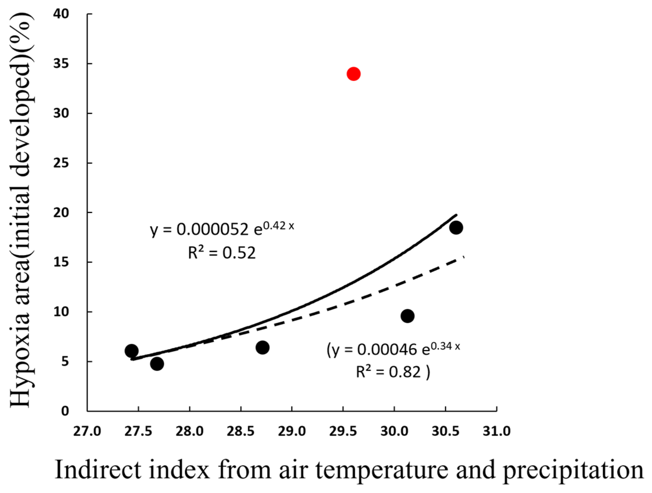
4.2. Prediction of Hypoxic Area from Weather Parameters

To assess the possibility of hypoxia prediction using weather parameters, the average weekly air temperature and total precipitation over 2–4 weeks before hypoxia, which are weather parameters significantly associated with the hypoxia indices (Table 6), were used as the reference parameters.

The conditions for hypoxia development during the period of 2011–2016 indicated that hypoxia developed when the average weekly air temperature was ≥19.5 °C and the total precipitation for 4 weeks was >100 mm, with exceptions in 2012 for the total precipitation (73 mm) and in 2015 for the weekly temperature (18.4 °C). Based on this finding, the area of initial hypoxia development could be predicted using the relationship between the air temperature and total precipitation, expressed as a simple equation (Equation (1), Figure 8):

Y = 0.0000524exp (0.4196X)
(if, excluding the case of 2014, Y = 0.0004657exp (0.33738X))
X = Temp_1w + ln (Precip_4w) × 1.8

(1)

where Y is the hypoxic area (%), Temp_1w is the average weekly air temperature, and Precip_4w is the total precipitation over 4 weeks. When 2014 was excluded, the correlation coefficient increased (R² = 0.82) compared to the whole period of 2011–2016 (R² = 0.52). This equation indicates that the initial occurrence of hypoxia and its initial area are determined by the development of stratification, which, in turn, is driven by the increasing temperature from spring to summer, followed by the intensification of stratification and eutrophication due to the freshwater inflow via rainfall.

As shown in Equation (1), the relationship of the initial occurrence of hypoxia with temperature suggests that its occurrence will accelerate with climate change. In reality, the timing of the initial development and expansion of hypoxia in Jinhae Bay showed earlier and larger changes than in the 1980s, when hypoxia began in mid-July and occurred only in the sub-bays of Masan Bay and Wonmun Bay [6,29]. These results are consistent with the findings of Diaz and Rosenberg [7], who revealed that oceanic oxygen decreases due to the intensification of stratification, increasing water temperature, and changing rainfall patterns. Furthermore, the long-term temperature trend at the Changwon Meteorological Center shows that the monthly average temperature in May is gradually rising, with the 10-year moving average showing a distinct increasing tendency (R² = 0.45). Thus, if the initial period of hypoxia occurrence in Jinhae Bay is expected to shift with climate change, then the temperature of the hypoxia initiation based on this scenario is approximately 19.5 ± 0.5 °C.

To investigate the conditions for hypoxia persistence over >50% of the development area after hypoxia initiation, 16 cases of hypoxia initiation and development from 2011 to 2016 were examined. Excluding September 2016, an occurrence area of hypoxia of ≥50% showed a positive logarithmic correlation with the four-week total rainfall (R² = 0.6, Figure 9). This result indicates that a close relationship exists between expansion or intensification after the first occurrence of hypoxia and the nutrients supplied by heavy rainfall. In particular, the hypoxic area peaks 1–2 times during every hypoxia season (Figure 7), and the correlation between the occurrence area and rainfall during these peak periods showed a strong logarithmic correlation (R² = 0.82) (Figure 9). Additionally, when the occurrence area was approximately 70% or greater, the four-week total rainfall was at least 250 mm. In September 2016, the four-week rainfall sum was approximately 510 mm, which was similar to that in September 2014, when the rainfall was the highest (511 mm); however, the associated hypoxic area was 57%, which was lower than in 2014 (71%). The hypoxic area was maximized in July 2016, gradually reduced to 20% at the beginning of September, and then expanded to ≥50% due to abundant rainfall. Therefore, after heavy rainfall, the increase in the hypoxic area was 37% (the area increased by 150 ha), which was larger than the 27% increase observed in 2014 (the area increased by 110 ha).

In 2014, despite the lowest monthly average temperature for August of the study period (24.6 °C), a hypoxic area of 70% was maintained through mid-September, as the cumulative rainfall in August was the greatest of the study period (666 mm). However, despite the monthly average temperature in August 2013 being the highest (28.0 °C), the cumulative rainfall was the lowest, at 82 mm. The smallest maximum occurrence area was 52%, and the overall hypoxic area was small in this case. Compared to the initial occurrence conditions supporting hypoxia, the maintenance condition (≥50%) was associated with a single criterion, requiring approximately 60% or more of the initial rainfall requirement. During the maintenance period, the atmospheric and water temperatures naturally increase after the initial occurrence of hypoxia from late spring to early summer; therefore, the condition of stratification is continuously satisfied. The supply of organic matter provides fuel that accelerates the oxygen consumption and is the most important factor for the intensification and maintenance of hypoxia.

Based on the relationships of the initiation and persistence of hypoxia with the air temperature and rainfall, some conditions of the air temperature and rainfall occurred repeatedly over the hypoxia seasons of 2011–2016:

Y = 15.26X_1w − 282.31
X = Temp_1w + ln (Precip_2~4w) × 1.25

(2)

where Y is the hypoxic area (%), Temp_1w is the average weekly air temperature, Precip_2~4w is the total precipitation before 2–4 weeks, and X_1w is the weekly average of X.

As described in Equation (2), the combination of the one-week average of the air temperature and total rainfall 2–4 weeks prior showed a significant positive linear relationship with the hypoxic area (R² = 0.56, Figure 10A). In contrast to the initial development, rainfall during the 1 week prior to analysis was excluded, as the 4-week sum of rainfall showed a weaker correlation than the sum for 2–4 weeks prior, suggesting that the final week of rainfall had little impact on the hypoxic area. This finding is in accordance with the one-month gap noted above between the heavy rainfall and the expansion of the hypoxic area. This relationship was employed to predict the hypoxic area for 2017–2020 using only weather parameters based on the daily air temperature and rainfall. A significant alignment between the predicted and observed hypoxic areas was obtained for these years (R² = 0.53, Figure 10B). However, the prediction for late July through early August differed somewhat from the observed area, with much smaller or larger areas (±30–50%). There are several possible reasons for this discrepancy. First, as the period of stratification coincides with the season of rapid warming, the air temperature alone cannot readily explain the strength of the stratification. In addition, this equation does not consider hypoxic areas that are already present, and thus the initial hypoxic area developed from June to July is excluded. Better predictions may be obtained through the application of modeling or deep learning methods rather than the linear-least-square method applied here. This study focused on identifying the relationships between oceanic and meteorological data and hypoxia to evaluate its direct and indirect causes and, thus, to assess the predictability of the development, persistence, and coverage of hypoxia in Jinhae Bay.

5. Conclusions

In Jinhae Bay, a famous area for hypoxia development every summer in Korea, we surveyed the environmental and meteorological parameter and hypoxia patterns from 2011 to 2016 and evaluated the major factors that affect the hypoxia occurrence and persistence to prevent fishery damage by predicting the hypoxia in the future.

Correlation analyses of the seawater properties, weather parameters, and hypoxia indices suggest that the air temperature and precipitation may be important factors that influence the development and persistence of hypoxia in Jinhae Bay by controlling the stratification intensity and eutrophication of the water column. From the results, the following trends of hypoxia in Jinhae Bay were revealed: the initial hypoxia development generally depends on the criteria of an air temperature ≥ 19.5 °C for 1 week and total precipitation > 100 mm over 4 weeks, and it becomes more severe (≥50% coverage) under strong eutrophication, mainly due to the organic matter discharge following heavy rainfall, based on a logarithmic correlation with the 4-week rainfall (R² = 0.6). Therefore, the hypoxic area index can be predicted using its linear regression relationships with the 1-week air temperature and 4-week precipitation (R² = 0.56). The relationship between the hypoxia area and weather parameters was applied for the 2017–2020 hypoxia season and also showed a significant correlation (R² = 0.53). This study tested the prediction of the hypoxic area based on a simple calculation method and weather parameter criteria, and it demonstrated the potential of this method for precisely forecasting hypoxia in combination with biogeochemical models or other mathematical solutions to prevent massive fishery damage.

References

1. Gray, J.S.; Wu, R.S.; Or, Y.Y. Effects of hypoxia and organic enrichment on the coastal marine enrichment. Mar. Ecol. Prog. Ser. 2022, 238, 249–279. [Google Scholar] [CrossRef]
2. Keiyu, M.; Yokota, M. Review on the hypoxia formation and its effects on aquatic organisms. Rep. Mar. Ecol. Res. Inst. 2012, 15, 1–21. [Google Scholar]
3. Saha, N.; Koner, D.; Sharma, R. Environmental hypoxia: A threat to the gonadal development and reproduction in bony fishes. Aquac. Fish. 2022, 7, 572–582. [Google Scholar] [CrossRef]
4. Rabalais, N.N.; Diaz, R.J.; Levin, L.A.; Turner, R.E.; Gilbert, D.; Zhang, J. Dynamics and distribution of natural and human-caused hypoxia. Biogeosciences 2010, 7, 585–619. [Google Scholar] [CrossRef]
5. Caballero-Alfonso, A.M.; Carstensen, J.; Conley, D.J. Biogeochemical and environmental drivers of coastal hypoxia. J. Mar. Syst. 2015, 141, 190–199. [Google Scholar] [CrossRef]
6. Lee, J.; Park, K.T.; Lim, J.H.; Yoon, J.E.; Kim, I.N. Hypoxia in Korea Coastal Waters: A Case Study of the Nutural Jinhae Bay and Artificial Shihwa Bay. Front. Mar. Sci. 2018, 5, 70. [Google Scholar] [CrossRef]
7. Diaz, J.R.; Rosenberg, R. Spreading Dead Zone and Consequences for Marine Ecosystems. Science 2008, 321, 926. [Google Scholar] [CrossRef]
8. Donald, W.S.; Scott, W.N. Stratification and Bottom-Water Hypoxia in the Pamlico River Estuary. Estuaries 1992, 15, 270–281. [Google Scholar]
9. Wiseman, W.J.; Rabalais, N.N.; Turner, R.E.; Dinnel, S.P.; MacNaughton, A. Seasonal and interannual variability within the Louisiana coastal current: Stratification and hypoxia. J. Mar. Syst. 1997, 12, 237–248. [Google Scholar] [CrossRef]
10. Kasai, A.; Yamada, T.; Takeda, H. Flow structure and hypoxia in Hiuchi-nada, Seto Inland Sea. Estuar. Coast. Shelf Sci. 2007, 71, 210–217. [Google Scholar] [CrossRef]
11. Chen, X.; Shen, Z.; Li, Y.; Yang, Y. Physical controls of hypoxia in waters adjacent to the Yangtze Estuary: A numerical modeling study. Mar. Pollut. Bull. 2015, 97, 349–364. [Google Scholar] [CrossRef] [PubMed]
12. Djakovac, T.; Supic, N.; Aubry, F.B.; Degobbis, D.; Giani, M. Mechanisms of hypoxia frequency changes in the northern Adriatic Sea during the period 1972–2012. J. Mar. Syst. 2015, 141, 179–189. [Google Scholar] [CrossRef]
13. Turner, R.E.; Rabalais, N.N.; Justić, D. Predicting summer hypoxia in the northern Gulf of Mexico: Riverine N, P, and Si loading. Mar. Pollut. Bull. 2006, 52, 139–148. [Google Scholar] [CrossRef]
14. Turner, R.E.; Rabalais, N.N.; Justić, D. Predicting summer hypoxia in the northern Gulf of Mexico: Redux. Mar. Pollut. Bull. 2012, 64, 319–324. [Google Scholar] [CrossRef] [PubMed]
15. Simon, D.D.; Donald, S. How climate controls the flux of nitrogen by the Mississippi River and the development of hypoxia in the Gulf of Mexico. Limnol. Oceanogr. 2007, 52, 856–861. [Google Scholar]
16. Testa, J.M.; Kemp, W.M. Hypoxia-induced shifts in nitrogen and phosphorus cycling in Chesapeake Bay. Limnol. Oceanogr. 2012, 57, 835–850. [Google Scholar] [CrossRef]
17. Meier, H.E.M.; Andersson, H.C.; Eilola, K.; Gustafsson, B.G.; Kuznetsov, I.; Müller-Karulis, B.; Neumann, T.; Savchuk, O.P. Hypoxia in future climates: A model ensemble study for the Baltic Sea. Geophys. Res. Lett. 2011, 38, L24608. [Google Scholar] [CrossRef]
18. Feng, Y.; DiMarco, S.F.; Jackson, G.A. Relative role of wind forcing and riverine nutrient input on the extent of hypoxia in the northern Gulf of Mexico. Geophys. Res. Lett. 2012, 39, L09601. [Google Scholar] [CrossRef]
19. Del Giudice, D.; Matli, V.R.R.; Obenour, D.R. Bayesian mechanistic modeling characterizes Gulf of Mexico hypoxia: 1968–2016 and future scenarios. Ecol. Appl. 2020, 30, e02032. [Google Scholar] [CrossRef]
20. Schourup-Kristensen, V.; Larsen, J.; Maar, M. Drivers of hypoxia variability in a shallow and eutrophicated semi-enclosed fjord. Mar. Pollut. Bull. 2023, 188, 114621. [Google Scholar] [CrossRef]
21. Roman, M.R.; Brandt, S.B.; Houde, E.D.; Pierson, J.J. Interactive effects of hypoxia and temperature on coastal pelagic zooplankton and fish. Front. Mar. Sci. 2019, 6, 139. [Google Scholar] [CrossRef]
22. Zhan, Y.; Ning, B.; Sun, J.; Chang, Y. Living in a hypoxia world: A review of the impacts of hypoxia on aquaculture. Mar. Pollut. Bull. 2023, 194, 115207. [Google Scholar] [CrossRef] [PubMed]
23. Kim, J.-H. Cross-sectional velocity variability and tidal exchange in a bay. Bull. Korean Fish. Tech. Soc. 1990, 26, 353–359. [Google Scholar]
24. Cho, C.H. Mass mortalities of oyster due to red tide in Jinhae Bay in 1978. Korean J. Fish. Aquat. Sci. 1979, 12, 27–33. [Google Scholar]
25. Kim, D.S.; Lee, C.W.; Choi, S.H.; Kim, Y.O. Long-term Changes in Water Quality of Masan Bay, Korea. J. Coast. Res. 2012, 28, 923–929. [Google Scholar] [CrossRef]
26. Kwon, J.N.; Lim, J.H.; Shim, J.; Lee, J.; Choi, T.J. The long-term variations of water quality in Masan Bay, South Sea of Korea. J. Korean Soc. Mar. Environ. 2014, 19, 212–223. [Google Scholar] [CrossRef]
27. Kim, Y.J.; Kim, M.K.; Yoon, J.S. Study of Formation and Development of Oxygen Deficient Water Mass, Using Ecosystem Model in Jinhae, Masan Bay. J. Ocean Eng. Technol. 2010, 24, 41–50. [Google Scholar]
28. MOF (Ministry of Oceans and Fisheries). Standard Method for the Analysis of Marine Environment. Available online: https://www.law.go.kr/admRulLsInfoP.do?admRulSeq=2000000109042 (accessed on 30 December 2020).
29. NFRDI. Hypoxic Water Masses in the Coast of Korea; GMK Communication Press: Busan, Republic of Korea, 2009; 173p.
30. Ferland, J.; Gosselin, M.; Starr, M. Environmental control of summer primary production in the Hudson Bay system: The role of stratification. J. Mar. Syst. 2011, 88, 385–400. [Google Scholar] [CrossRef]
31. He, B.; Dai, M.; Zhai, W.; Guo, X.; Wang, L. Hypoxia in the upper reaches of the Pearl River estuary and its maintenance mechanisms: A synthesis based on multiple year observations during 2000–2008. Mar. Chem. 2014, 167, 13–24. [Google Scholar] [CrossRef]
32. Huang, Y.; An, S. Weak hypoxia enhanced denitrification in a dissimilatory nitrate reduction to ammonium(DNRA)-dominated shallow and eutrophic coastal waterbody, Jinhae Bay, South Korea. Front. Mar. Sci. 2022, 9, 897474. [Google Scholar] [CrossRef]
33. Park, Y.; Cha, J.; Song, B.; Huang, Y.; Kim, S.; Kim, S.; Jo, E.; Fortin, S.; An, S. Total microbial activity and sulfur cycling microbe changes in response to the development of hypoxia in a shallow estuary. Ocean Sci. J. 2020, 55, 165–181. [Google Scholar] [CrossRef]
34. Keeling, R.F.; Körtzinger, A.; Gruber, N. Ocean deoxygenation in a warming world. Annu. Rev. Mar. Sci. 2010, 2, 463–493. [Google Scholar] [CrossRef] [PubMed]
35. Alvisi, F.; Cozzi, S. Seasonal dynamics and long-term trend of hypoxia in the coastal zone of Emilia Romagna (NW Adriatic Sea, Italy). Sci. Total Environ. 2016, 541, 1448–1462. [Google Scholar] [CrossRef] [PubMed]
36. Rabalais, N.N.; Turner, R.E.; Sen Gupta, B.K.; Boesch, D.F.; Chapman, P.; Murrell, M.C. Hypoxia in the northern Gulf of Mexico: Does the science support the plan to reduce, mitigate, and control hypoxia? Estuaries Coasts 2007, 30, 753–772. [Google Scholar] [CrossRef]
37. Wang, P.; Wang, H.; Linker, L.; Hinson, K. Influence of wind strength and duration on relative hypoxia reductions by opposite wind directions in an estuary with an asymmetric channel. J. Mar. Sci. Eng. 2016, 4, 62. [Google Scholar] [CrossRef]
Figure 1. Study area and sampling stations in Jinhae Bay, Korea, from 2011 to 2016 (blue squares: 2011–2012; red dots: 2013–2016; green circles: eight representative stations).
Jmse 12 00014 g001
Figure 2. Horizontal distribution of water temperature (°C) in Jinhae Bay from 2011 to 2016 (upper: surface water; lower: bottom water).
Jmse 12 00014 g002aJmse 12 00014 g002b
Figure 3. Horizontal distribution of salinity in Jinhae Bay from 2011 to 2016 (upper: surface water; lower: bottom water).
Jmse 12 00014 g003aJmse 12 00014 g003b
Figure 4. Horizontal distribution of dissolved oxygen (mg/L) in Jinhae Bay from 2011 to 2016 (upper: surface water; lower: bottom water).
Jmse 12 00014 g004
Figure 5. Horizontal distribution of hypoxia in bottom water of Jinhae Bay from 2011 to 2016. Black digits are areas (km2) of hypoxia development at each month and blue numbers are the area percentages (%) of hypoxia to the green square in the upper-most left image (34.85~35.25° N, 128.4~128.7° E).
Jmse 12 00014 g005
Figure 6. Temporal variations in vertical DO profiles at stations of Dangdong–Wonmun (A), Gajo (B), and Chilcheon (C) from 2011 to 2016.
Jmse 12 00014 g006
Figure 7. Temporal variations in daily air temperature (red lines) and precipitation (blue bars, right scale) measured at Changwon meteorological station, and hypoxia area (%, grey area, second right scale) in Jinhae Bay from 2011 to 2016.
Jmse 12 00014 g007
Figure 8. Relationship between hypoxia area for initial stage and indirect index calculated from air temperature and precipitation using Equation (1). Dashed regression line is applied for the case of excluding 2014 (red dot).
Jmse 12 00014 g008
Figure 9. Hypoxia areas for all surveyed cases (A) and for peaked cases (B) as a function of the sum of precipitation before 4 weeks, where dotted lines represent logarithmic correlations.
Jmse 12 00014 g009
Figure 10. Hypoxia area from 2011 to 2016 as a function of the 1–week average of X in Equation (2) (A), and calculated hypoxia area as a function of the observed from 2017 to 2020 (B). The dotted lines in (A,B) represent linear least-square fits.
Jmse 12 00014 g010