The Mitigation of Mutual Coupling Effects in Multi-Beam Echosounder Calibration under Near-Field Conditions

Abstract

The advancement of unmanned platforms is driving the miniaturization and cost reduction of the multi-beam echosounder (MBES). In the process of MBES array calibration, the mutual coupling significantly impacts the performance of parameter estimation. We propose a correction method to mitigate the mutual coupling effects in the calibration of MBES acoustic array. Initially, a near-field focused beamforming model is established to assess the influence of mutual coupling. Subsequently, the covariance matrix in the frequency domain is constructed to enhance algorithm efficiency and simplify solution procedures. This construction eliminates the need for a low-pass filtering step after heterodyning through extracting peak values near zero frequency in the signal frequency domain. Meanwhile, the Toeplitz property is leveraged to render the estimation results independent of the mutual coupling matrix. Finally, the mutual coupling coefficients and the direction of arrival (DOA) are joint-estimated and the Cramér–Rao bound is derived. The presented method effectively addresses the engineering challenge of MBES mutual coupling calibration. Additionally, the performance of the proposed method is verified through the measured data in simulation and tank experiments.

1. Introduction

Multi-beam echosounder (MBES) holds significant potential across various fields, including marine science, resource exploration and environmental monitoring [1,2,3]. It serves as an essential instrument for conducting deep-sea research and ocean engineering, offering a crucial window into the mysteries of the underwater world. In the context of seabed terrain detection using a MBES, precise calibration of the transducer array is imperative to ensure accurate measurements. This calibration process encompasses amplitude and phase adjustments, as well as addressing mutual coupling errors. The growing prevalence of unmanned technology necessitates a substantial quantity of cost-effective equipment. Consequently, the adoption of more efficient calibration techniques can enhance both cost-effectiveness and scalability [4,5]. Especially in array signal processing with a limited number of elements, calibrating the mutual coupling effect is of significance.

Mutual coupling errors are prevalent in multi-channel arrays due to inevitable coupling effects between channels stemming from hardware circuits or other sources, and they exert an adverse impact on parameter estimation [6,7,8]. Of particular significance is their detrimental effect on the direction of arrival (DOA) performance [9,10]. When a signal traverses through one element, it introduces interference to adjacent array elements, resulting in output errors. To effectively suppress mutual coupling errors, various strategies can be considered, including the optimization of circuitry and array layout [11,12], along with the implementation of shielding or isolation measures. Researchers such as Liu et al. [13] and Mei et al. [14] have pioneered the development of a novel array configuration known as the super nested sparse array, which combines the advantages of sparse arrays while significantly reducing mutual coupling effects. Additionally, a symmetric thinned coprime array (STCA), consisting of two sparse uniform linear arrays, has been demonstrated to mitigate mutual coupling in mixed source localization scenarios [14]. However, the performance of the algorithm is often degraded under the influence of pulse noise. To overcome this problem, Zhang et al. proposed an improved algorithm to reconstruct the sparse model and achieve accurate DOA estimation [7]. This menthod involves creating a sparse representation of received signals through the mutual coupling matrix (MCM) structure and Cauchy-score-based cost function.

Nevertheless, once the array structure is determined, signal processing methods become the prevalent approach for estimating and compensating for mutual coupling errors. Calibration methods fall into two broad categories: active calibration and self-calibration, depending on the presence or absence of auxiliary signal sources. Active calibration is theoretically feasible [15]. However, in practical applications, it may introduce manual errors due to the challenge of accurately obtaining signal source information, thereby potentially affecting calibration accuracy. In contrast, self-calibration methods offer the advantage of not relying on auxiliary signal sources.

The mutual coupling model, though inherently complex, can be simplified in certain cases [16,17]. By conceptualizing angularly independent mutual coupling as angularly dependent complex array gains, Liao et al. [18] identified a remarkable property where the middle subarray exhibits identical complex array gains. Leveraging this insight, a MCM was developed using complete array data, guided by the subspace principle. It is worth noting that mutual coupling can also be transformed into amplitude and phase errors [19]. Gain errors are estimated using the main diagonal of the actual covariance matrix of the virtual uniform linear array (ULA), while phase errors can be determined through the Toeplitz structure of the ideal covariance matrix [20]. The symmetric Toeplitz structure of the MCM plays a crucial role in solving these challenges [21]. Wang et al. [22] employed reweighted ${𝓁}_1$-norm minimization with error-constrained ${𝓁}_2$-norm to enhance sparsity and robustness against noise, enabling DOA estimation without mutual coupling compensation. In addition to these methods, alternative approaches to DOA estimation with mutual coupling involve creating a new spectral estimation function from a subspace perspective. Weighted matrices based on a MUSIC-like function were constructed to address this issue [23]. Wang [24] utilized a reweighted ${𝓁}_1$-norm minimization scheme to recover a block-sparse matrix, forming a MUSIC-like spectrum function that enhances DOA estimation performance with mutual coupling.

It is important to note that the above-mentioned methods predominantly focus on calibrating mutual coupling errors in radar antenna arrays and assume far-field conditions. The advancement of unmanned platforms has led to the miniaturization and cost reduction of MBES, diminishing array complexity. Nevertheless, there remains a demand for high accuracy in DOA estimation. Therefore, it is particularly important for MBES array calibration. However, when calibrating a MBES in a water tank, the system often operates in a near-field environment. Following calibration, mutual coupling compensation is performed on each channel of the array to ensure consistency between the array elements. Consequently, real-time DOA estimation under mutual coupling conditions is no longer necessary during the practical application of the MBES.

This paper introduces a self-calibration algorithm that relies on near-field focused beamforming models to mitigate mutual coupling errors between channels in MBES. The algorithm leverages the Toeplitz property of the mutual coupling matrix to facilitate mutual coupling calibration. Through the use of a transformation matrix, the algorithm reshapes the array manifold affected by mutual coupling into a new manifold. Subsequently, it computes an independent spectral function devoid of mutual coupling effects.

The remainder of this paper is structured as outlined below. Section 2 introduces the near-field focused beamforming model and the signal model of a ULA. The proposed correction method is presented and described in Section 3. Section 4 shows the experimental results and engages in subsequent discussions. Finally, the conclusion is drawn in Section 5.

2. Analysis of DOA Estimation in the Context of Mutual Coupling

Licitra et al. provides a comprehensive review of state-of-the-art beamforming algorithms employed in the estimation of DOA, covering both theoretical underpinnings and practical applications [25]. These algorithms can be broadly categorized into six distinct groups: conventional beamforming, functional beamforming, adaptive beamforming, eigenvalue decomposition, deconvolution methods and holographic methods [26,27,28].

This study concentrates on the utilization of a ULA within a MBES as the primary receiving array. The ULA comprises lots of elements that form an extremely narrow beam, resulting in better angular resolution and higher array gain. Conventional methods usually have no limitation on the size of the experimental tank and are mainly suitable for arrays with a large number of elements. Unlike conventional approaches, this research employs the near-field propagation model to effectively overcome these limitations. In conclusion, this study demonstrates the advantages of employing the near-field propagation model for improving the performance of the ULA within MBES, particularly in scenarios with size constraints.

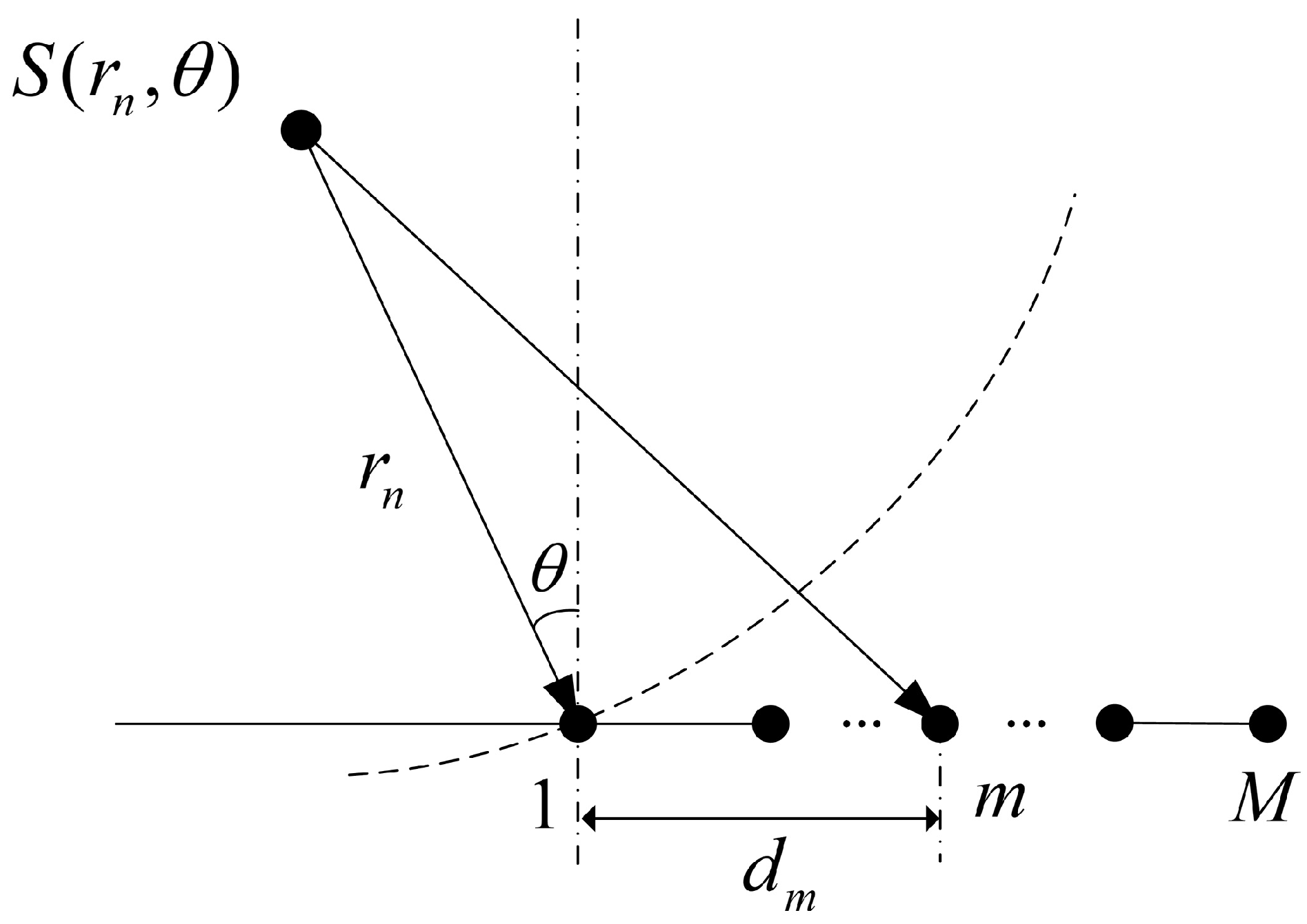
2.1. Near-Field Focused Beamforming Model

Near-field focused beamforming technology utilizes sensor arrays and phase control to focus the beam in the direction of the target to enhance the signal and suppress interference, with a wide range of applications in sonar imaging systems. The distance between the source and the array should satisfy the following equation:

$$r<\frac{2D^2}{\lambda },$$

(1)

where D represents the scale of the array and $\lambda$ represents the acoustic wavelength. It is important to note that employing the plane wave model under these conditions significantly impairs array performance [29].

The relevant parameters of the receiving array with M elements are shown in Figure 1. The element spacing, denoted as $d=\lambda /2$, where $\lambda$ represents the wavelength of the acoustic wave. The speed of sound transmission in water, represented as c, and the center frequency of the echo, denoted as f, are crucial factors. The Fresnel approximation is employed to enhance the steering vector. The phase difference between the first and $m$th array element can be expressed as follows [30]:

$${\varphi }_m(r,\theta )\approx -2\pi dsin\frac{\theta }{\lambda }+\pi d_m^{2}co{s}^2\frac{\theta }{\lambda r},$$

(2)

where r represents the focal distance, $\theta$ denotes the beam angle under consideration and $d_m$ signifies the distance between the first and $m$th array element. Unlike far-field beamforming, near-field beamforming must consider the focal distance. Equation (2) becomes conventional beamforming when the second entry is omitted. Furthermore, far-field beamforming can be viewed as an approximation of near-field calculations. The real-time analysis of focusing beamforming at each sampling interval can be represented as:

$$\mathbf{V}\left(r,\theta \right)=\sum _{m=0}^{M-1}{x}_m(\cos \left({\phi }_m\right)-j\sin \left({\phi }_m\right)),$$

(3)

where $x_m$ represents the received signal at the $m$th element.

2.2. The Signal Model

Consider a ULA comprising M elements subjected to the influence of N narrowband signals arriving from distinct directions, denoted as ${\theta }_i$ for $i=1,2,\dots ,N$, assuming that the incident signals are mutually independent, as are the signal and noise. Consequently, the output signal of the receiving array is as follows:

$$\mathbf{X}\left(t\right)=\mathbf{A}\mathbf{S}\left(t\right)+\mathbf{n}\left(t\right),$$

(4)

where $\mathbf{X}\left(t\right)={\left[x_1\left(t\right),x_2\left(t\right),\dots ,x_M\left(t\right)\right]}^T$ is an $M\times 1$ receiving signal matrix and $S\left(t\right)$ is an $N\times 1$ matrix whose elements are high frequency cosine signals. ${\mathbf{A}}^{M\times N}$ consists of diagonal elements corresponding to the array steering vectors and can be expressed as follows:

$$\mathbf{A}=[\mathbf{a}(r_1,{\theta }_1)\mathbf{a}(r_2,{\theta }_2)\cdots \mathbf{a}(r_N,{\theta }_N)],$$

(5)

where:

$$\mathbf{a}(r_n,{\theta }_n)=\left[\begin{array}{c}\begin{array}{c}\begin{array}{c}{a}_1\\ a_2\end{array}\\ \cdots \end{array}\\ a_M\end{array}\right]=\left[\begin{array}{c}\begin{array}{c}\begin{array}{c}{e}^{-j{\phi }_1(r_n,{\theta }_n)}\\ e^{-j{\phi }_2(r_n,{\theta }_n)}\end{array}\\ \cdots \end{array}\\ e^{-j{\phi }_M(r_n,{\theta }_n)}\end{array}\right],$$

(6)

In Equation (4), ${\mathbf{n}}^{M\times 1}\left(t\right)$ represents the noise matrix. It is assumed that the noise across channels is uncorrelated and exhibits equal variance. It is well-established that the steering vector $\mathbf{a}(r,\theta )$ is susceptible to the influence of neighboring elements when mutual coupling is present. This phenomenon can be characterized as follows:

$$\tilde{\mathbf{a}}(r,\theta )=\mathbf{Ca}(r,\theta ),$$

(7)

where $\mathbf{C}$ denotes the MCM, which can be approximated by a p-banded Toeplitz matrix in the ULA configuration and takes the following form:

$$\mathbf{C}={\left[\begin{array}{cccccc}1& c_1& \cdots & c_{p-1}& \cdots & c_{M-1}\\ c_1& 1& c_1& \cdots & \ddots & ⋮\\ ⋮& c_1& 1& c_1& \cdots & c_{p-1}\\ c_{p-1}& \cdots & \ddots & \ddots & \ddots & ⋮\\ ⋮& \ddots & \cdots & c_1& 1& c_1\\ c_{M-1}& \cdots & c_{p-1}& \cdots & c_1& 1\end{array}\right]}_{M\times M},$$

(8)

where $c_i$ represents the mutual coupling coefficients, defined as $c_i={\rho }_i{e}^{j{\varphi }_i}(i=1,2,\cdots ,M)$, where ${\rho }_i$ and ${\varphi }_i$ are the amplitude and phase of $c_i$. It has been empirically observed that $c_i$ behaves as functions of inter-sensor spacing, being inversely proportional to their distance. When the distance between two elements exceeds p inter-sensor spacing, $c_i$ becomes approximately 0, that is:

$$c_i=0,p\le i\le M-1,$$

(9)

3. Proposed Correction Method for MBES Receiving Arrays

3.1. Mathematic Model

When accounting for mutual coupling, the covariance matrix of the output signal can be expressed as:

$$\tilde{\mathbf{R}}=\mathbf{CA}{\mathbf{R}}_S{\mathbf{A}}^H{\mathbf{C}}^H+{\sigma }^2\mathbf{I},$$

(10)

where ${(·)}^H$ represents Hermitian transpose, ${\mathbf{R}}_S$ represents the signal covariance matrix and I represents the identity matrix and ${\sigma }^2$ denotes the noise power. Under the condition of uncorrelated source signals, where the rank of ${\mathbf{R}}_S$ is equal to N, ${\mathbf{R}}_S$ can be described as follows after eigendecomposition:

$$\tilde{\mathbf{R}}={\mathbf{U}}_S{\mathbf{\Sigma }}_S{\mathbf{U}}_S^H+{\mathbf{U}}_V{\mathbf{\Sigma }}_V{\mathbf{U}}_V^H,$$

(11)

where ${\mathbf{U}}_S\in \mathbb{C}{}^{M\times N}$ and ${\mathbf{U}}_V\in \mathbb{C}{}^{M\times (M-N)}$ represent the signal and noise subspaces, respectively. Additionally, ${\mathbf{\Sigma }}_S\in \mathbb{R}{}^{M\times M}$ and ${\mathbf{\Sigma }}_V\in \mathbb{R}{}^{(M-N)\times (M-N)}$ are diagonal matrices related to signal and noise power, respectively.

In particular, the specific derivation of the estimation of the receiver covariance matrix is not described here, and it can be viewed in previous studies [20]. It can be denoted as:

$${\widehat{\mathbf{R}}}_X={\mathbf{X}}_P^T{\mathbf{X}}_P,$$

(12)

where the plural vector ${\mathbf{X}}_P={[P_1,P_2,\cdots ,P_M]}^T$.

3.2. Algorithm Principle

The solution for the mutual coupling matrix $\mathbf{C}$ can be reformulated as an optimization problem rooted in subspace theory, aiming to minimize the cost function, $f(r,\theta ,c)$, denoted as:

$$f(r,\theta ,c)=\min {∥\left(\mathbf{Ca}(r,\theta )\right){\widehat{\mathbf{U}}}_V∥}^2=\min {∥\left(\tilde{\mathbf{a}}(r,\theta )\right){\widehat{\mathbf{U}}}_V∥}^2,$$

(13)

where ${\widehat{\mathbf{U}}}_V$ signifies the estimation of the noise space within ${\mathbf{U}}_V$. To address this, we reformulate the mutual coupling component of Equation (13) using the mutual coupling vector $\overline{\mathbf{c}}$. This vector is defined as $\overline{\mathbf{c}}=[c_1,c_2,\cdots ,c_p$ ] and corresponds to the non-zero elements of the mutual coupling coefficients $c_i$. Let $\mathbf{W}(r,\theta )$ be the transformation matrix associated with r and $\theta$. The steering vector with mutual coupling $\tilde{\mathbf{a}}(r,\theta )$ can be expressed as:

$$\tilde{\mathbf{a}}(r,\theta )=\mathbf{Ca}(r,\theta )=\mathbf{W}(r,\theta )\overline{\mathbf{c}},$$

(14)

where

$$\left.\begin{array}{c}{\mathbf{W}}_{i,j}(r,\theta )=\left\{\begin{array}{c}{a}_i,\\ a_{i+j-1}+a_{i-j+1},\end{array}\right.\begin{array}{c}j=1\\ 2\le j\le p\end{array}\hfill \\ i\in (1,2,\cdots M),j\in (1,2,\cdots p)\hfill \end{array}\right\},$$

(15)

In addition, a sequence $a_0=0$, $a_{-1}=a_{M+1}=0$, $a_{-2}=a_{M+2}=0$,…, $a_{-(p-1)}=a_{M+(p-1)}=0$ is defined. By substituting Equation (15) into Equation (14), its correctness can be verified. It is important to note that $\mathbf{W}(r,\theta )$ is independent of $\overline{\mathbf{c}}$. Furthermore, by substituting Equation Equation (15) into Equation (13), the cost function $f(r,\theta ,c)$ can be rewritten as follows:

$$\begin{array}{c}f(r,\theta ,c)=\min {∥{\left(\mathbf{W}(r,\theta )\overline{\mathbf{c}}\right)}^H{\mathbf{U}}_V∥}^2\hfill \\ =\min {\overline{\mathbf{c}}}^H\mathbf{W}(r,\theta ){\widehat{\mathbf{U}}}_V{\widehat{\mathbf{U}}}_V^H\mathbf{W}(r,\theta )\overline{\mathbf{c}}\hfill \\ =\min {\overline{\mathbf{c}}}^H\mathbf{Q}(r,\theta )\overline{\mathbf{c}}\hfill \end{array},$$

(16)

where $\mathbf{Q}(r,\theta )=\mathbf{W}(r,\theta ){\widehat{\mathbf{U}}}_V{\widehat{\mathbf{U}}}_V^H\mathbf{W}(r,\theta )$ and this independence holds for $\overline{\mathbf{c}}$ as well. The first element of vector $\overline{\mathbf{c}}$ is fixed at 1, and $\overline{\mathbf{c}}\epsilon =1$, where ${\mathbf{\epsilon }}^{p\times 1}={[1,0,\cdots ,0]}^T$. Consequently, the problem can be reformulated as a quadratic-linear problem, represented as:

$$\min {\overline{\mathbf{c}}}^H\mathbf{Q}(r,\theta )\overline{\mathbf{c}},s.t.{\mathbf{\epsilon }}^T\overline{\mathbf{c}}=1,$$

(17)

The Lagrange function $L(x,\lambda )$ can be established as:

$$L(x,\lambda )={\mathbf{x}}^H\mathbf{Q}(r,\theta )\mathbf{x}-\lambda ({\mathbf{\epsilon }}^T\mathbf{x}-1),$$

(18)

and set as:

$$\left\{\begin{array}{c}{\nabla }_{\mathbf{x}}L(\mathbf{x},\lambda )=0\\ {\nabla }_{\lambda }L(\mathbf{x},\lambda )=0\end{array}\right.,$$

(19)

where $\mathbf{x}=\overline{\mathbf{c}}$, and Equation (18) can be described as:

$$\left[\begin{array}{cc}{\mathbf{Q}}^H& -\mathbf{\epsilon }\\ -{\mathbf{\epsilon }}^T& \mathbf{0}\end{array}\right]\left[\begin{array}{c}\mathbf{x}\\ {\lambda }^H\end{array}\right]=\left[\begin{array}{c}0\\ -1\end{array}\right],$$

(20)

where $\lambda$ represents the Lagrange multiplier.

To facilitate the solution, construct the following formula:

$$\left[\begin{array}{cc}{\mathbf{Q}}^H& -\mathbf{\epsilon }\\ -{\mathbf{\epsilon }}^T& \mathbf{0}\end{array}\right]\left[\begin{array}{cc}{\mathbf{P}}^H& -\mathbf{R}\\ -{\mathbf{R}}^H& \mathbf{G}\end{array}\right]={\mathbf{I}}_{2p},$$

(21)

where ${\mathbf{I}}_{2p}$ represents the 2×p identity matrix and $\mathbf{G}$, $\mathbf{R}$, $\mathbf{P}$ are the matrices constructed during the derivation.

Given the reversibility of $\mathbf{Q}$ and the existence of its inverse matrix ${\mathbf{Q}}^H$, the matrices ${\mathbf{P}}^H$, ${\mathbf{R}}^H$ and $\mathbf{G}$ are described as:

$$\left\{\begin{array}{c}{\mathbf{P}}^H={\mathbf{Q}}^{-H}-{\mathbf{Q}}^{-H}\mathbf{\epsilon }{\left({\mathbf{\epsilon }}^T{\mathbf{Q}}^{-H}\mathbf{\epsilon }\right)}^{-1}{\mathbf{\epsilon }}^T{\mathbf{Q}}^{-H}\hfill \\ {\mathbf{R}}^H={\left({\mathbf{\epsilon }}^T{\mathbf{Q}}^{-H}\mathbf{\epsilon }\right)}^{-1}{\mathbf{\epsilon }}^T{\mathbf{Q}}^{-H}\hfill \\ \mathbf{G}=-{\left({\mathbf{\epsilon }}^T{\mathbf{Q}}^{-H}\mathbf{\epsilon }\right)}^{-1}\hfill \end{array}\right.,$$

(22)

where ${\mathbf{Q}}^{-H}$ represents the inverse matrix of ${\mathbf{Q}}^H$. By using Equations (20)–(22), $\mathbf{x}=\mathbf{R}$ can be derived, implying that:

$$\overline{\mathbf{c}}=\frac{{\mathbf{Q}}^{-1}(r,\theta )\mathbf{\epsilon }}{{\mathbf{\epsilon }}^T{\mathbf{Q}}^{-1}(r,\theta )\mathbf{\epsilon }},$$

(23)

where ${\mathbf{Q}}^{-1}$ represents the inverse matrix of $\mathbf{Q}$, when Equation (23) is substituted into the cost function $f(r,\theta ,c)$, a new spectral function is then obtained, $F\left(\theta \right)$, denoted as:

$$F\left(\theta \right)={\mathbf{\epsilon }}^T{\mathbf{Q}}^{-1}(r,\theta )\mathbf{\epsilon }=\det \left({\mathbf{Q}}_z\left(\theta \right)\right)/\det \left(\mathbf{Q}\left(\theta \right)\right),$$

(24)

where ${\mathbf{Q}}_z(r,\theta )$ represents as the subarray of $\mathbf{Q}$ encompassing rows from the second to the pth and columns from the second to the pth and $\det \left(\right)$ represents the determinant of the matrix Proceeding to investigate the maximum position of the spectral function F, the ranges and DOAs can be estimated. Furthermore, the mutual coupling vector $\overline{\mathbf{c}}$ can be calculated by substituting them into Equation (23), and subsequently, the mutual coupling matrix $\mathbf{C}$ is obtained. This is in accordance with the analysis and verification conducted by Qi et al. [31]. For the parameter p, it should satisfy the following criteria:

$$p\le \min \left(⌈M/\phantom{M2}2⌉,M-N\right),$$

(25)

where $⌈·⌉$ represents the integer ceiling operator. The proposed algorithm discussed above is summarized in

Table 1. Procedural steps for the proposed mutual coupling correction method.

Step	The Procedure of Concrete Operations in the Proposed Method
Step 1	A Fourier transform is applied to the output signal of each channel $\mathbf{X}\left(t\right)$ and the peak value ${\mathbf{X}}_P$ is established in the frequency domain.
Step 2	The covariance matrix ${\widehat{\mathbf{R}}}_X$ is computed according to Equation (12).
Step 3	Determine the subspace ${\widehat{\mathbf{U}}}_V$ using Equation (11).
Step 4	Define the mutual coupling vector $\mathbf{\epsilon }$.
Step 5	Establish the steering vector $\mathbf{a}(r,\theta )$ for each r and $\theta$.
Step 6	Formulate the transformation matrix $\mathbf{W}(r,\theta )$ based on Equation (17).
Step 7	Utilize $\mathbf{W}(r,\theta )$ and ${\widehat{\mathbf{U}}}_V$ to calculate $\mathbf{Q}(r,\theta )$, followed by the derivation of ${\mathbf{Q}}_z(r,\theta )$.
Step 8	Utilize Equation (24) to estimate the ranges and DOAs for N sources through the spectral function $F\left(\theta \right)$.
Step 9	Establish each ${\mathbf{Q}}_z(r,\theta )$ and compute MCM and $\overline{\mathbf{c}}$ as defined by Equations (8) and (23).

.

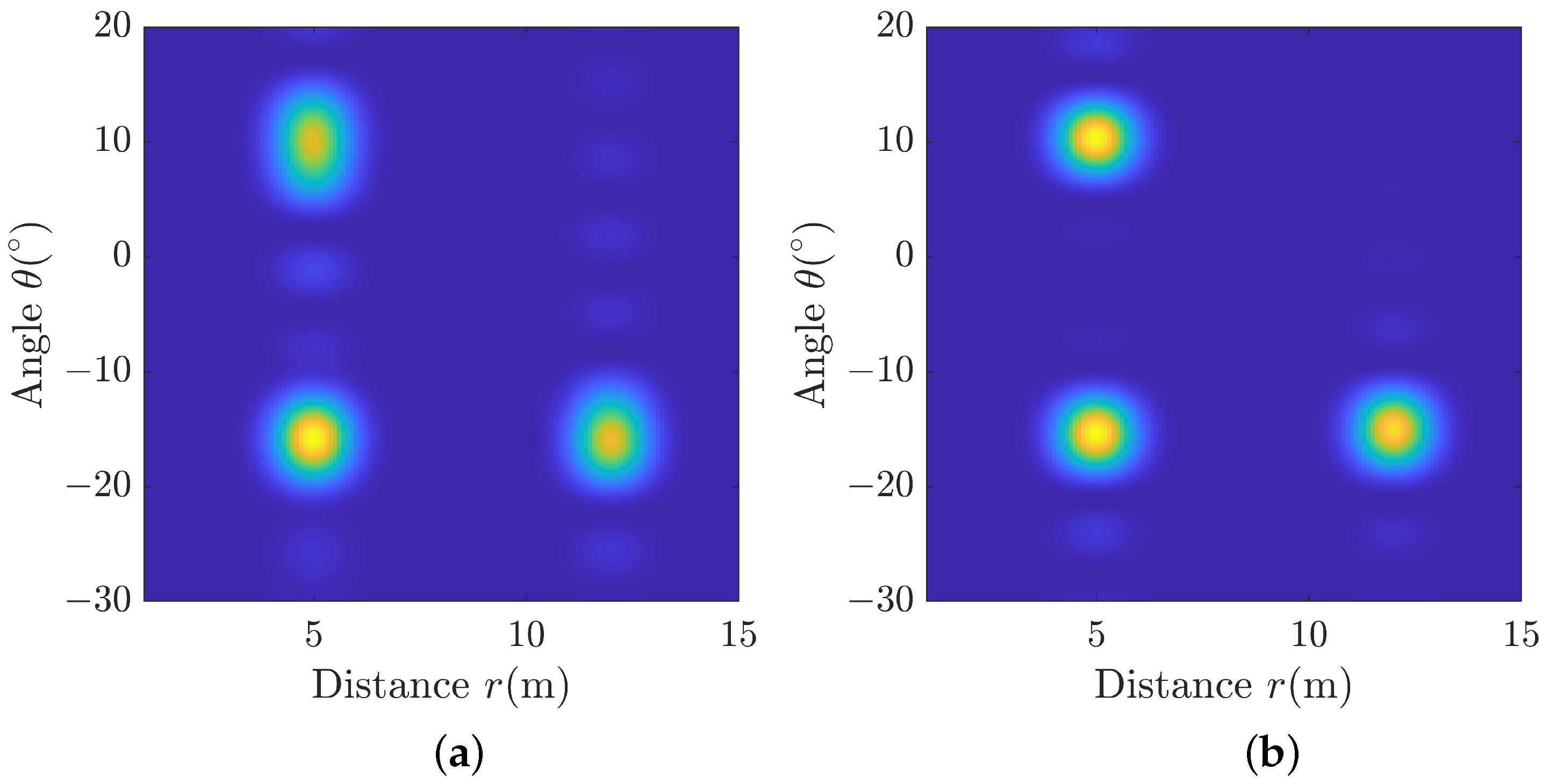
3.3. Performance of the Proposed Algorithm

Within the framework of the proposed algorithm, the real and imaginary components of the MCM can be treated as a collection of random variables, as outlined below:

$$\begin{array}{c}\mathbf{r}={[r_1,r_2,\cdots ,r_N]}^{\mathrm{T}}\hfill \\ \mathbf{\theta }={[{\theta }_1,{\theta }_2,\cdots ,{\theta }_N]}^{\mathrm{T}}\hfill \\ \mathbf{\rho }={[{\rho }_1,{\rho }_2,\cdots ,{\rho }_p]}^{\mathrm{T}}\hfill \\ \mathbf{\eta }={[{\eta }_1,{\eta }_1,\cdots ,{\eta }_p]}^{\mathrm{T}}\hfill \end{array},$$

(26)

where ${\mathit{\rho }}_{\mathit{i}}=\mathrm{Re}\left[c_i\right]$ and ${\mathit{\eta }}_{\mathit{i}}=\mathrm{Im}\left[c_i\right]$ denote the real and imaginary components of the mutual coupling coefficient, respectively. Subsequently, the Cramér–Rao bounds (CRB) for the joint estimation of each parameter are expressed as follows:

$$\mathbf{CRB}={\mathbf{F}}^{-1},$$

(27)

where $\mathbf{F}$ represents the Fisher information matrix, which can be expressed in block-wise manner as follows:

$$\mathbf{F}=\left[\begin{array}{cccc}{\mathbf{F}}_{\mathit{rr}}\hfill & {\mathbf{F}}_{\mathit{\theta }\mathit{r}}& {\mathbf{F}}_{\mathit{\rho }\mathit{r}}& {\mathbf{F}}_{\mathit{\eta }\mathit{r}}\\ {\mathbf{F}}_{\mathit{r}\mathit{\theta }}\hfill & {\mathbf{F}}_{\mathit{\theta }\mathit{\theta }}& {\mathbf{F}}_{\mathit{\rho }\mathit{\theta }}& {\mathbf{F}}_{\mathit{\eta }\mathit{\theta }}\\ {\mathbf{F}}_{\mathit{r}\mathit{\rho }}\hfill & {\mathbf{F}}_{\mathit{\theta }\mathit{\rho }}& {\mathbf{F}}_{\mathit{\rho }\mathit{\rho }}& {\mathbf{F}}_{\mathit{\eta }\mathit{\rho }}\\ {\mathbf{F}}_{\mathit{r}\mathit{\eta }}\hfill & {\mathbf{F}}_{\mathit{\theta }\mathit{\eta }}& {\mathbf{F}}_{\mathit{\rho }\mathit{\eta }}& {\mathbf{F}}_{\mathit{\eta }\mathit{\eta }}\end{array}\right],$$

(28)

where ${\mathbf{F}}_{\mathit{rr}}$ is the range estimation block and ${\mathbf{F}}_{\mathit{\theta }\mathit{\theta }}$ is the azimuth estimation block, ${\mathbf{F}}_{\mathit{\rho }\mathit{\rho }}$ and ${\mathbf{F}}_{\mathit{\eta }\mathit{\eta }}$ are the real part and imaginary part estimation blocks of matrix element mutual coupling coefficients, respectively. The others are the cross-correlation blocks estimated by the corresponding parameters.

4. Experimental Results

4.1. Mutual Coupling

The performance of the proposed method in this paper is assessed through simulation as follows. An array with $M=20$ elements and $N=3$ sources is considered. To assess the impact of mutual coupling on the estimation results for sources at the same direction or range, the source positions are defined as follows: $r_1=12$ m, ${\theta }_1=-15$°, $r_2=5$ m, ${\theta }_2=10$°, $r_3=5$ m, ${\theta }_3=-15$°.

The mutual coupling matrix is determined using Equation (8), while the mutual coupling vector is represented as $\overline{\mathbf{c}}=[1,0.9e^{j\pi },0.6e^{j0.7\pi },0.2e^{j0.4\pi },0.3e^{j0.5\pi }]$ and $p=5$. The angle resolution and range resolution are 0.1° and 0.1 m, respectively. The signal-to-noise ratio (SNR) is set to 20 dB. Figure 2 displays the near-field beamforming results, comparing those obtained with and without the application of the mutual coupling correction method proposed in this paper.

Following correction, the beam pattern’s quality experienced a marked enhancement, effectively mitigating the blurring issue observed prior to calibration. Furthermore, our observations indicate that mutual coupling errors among channels can lead to increased sidelobe occurrences in the near-field focused beamforming results across various incident angle directions, potentially impacting DOA estimation accuracy. Tabular data in

Table 2. The range and DOA estimation results under different conditions.

Source		Unknown Mutual Coupling	Proposed Method	Known Mutual Coupling
Source 1	Range	11.9 m	12.0 m	12.0 m
	DOA	$-15.8$°	$-15.0$°	$-15.0$°
Source 2	Range	5.0 m	5.0 m	5.0 m
	DOA	$8.9$°	$10.0$°	$10.0$°
Source 3	Range	4.9 m	5.0 m	5.0 m
	DOA	$-15.9$°	$-15.0$°	$-15.0$°

present the associated results for DOA and range detection. It can be inferred that mutual coupling predominantly affects DOA estimation and this influence can be corrected by the proposed method.

As an illustrative case, Source 2 is considered. Figure 3 shows the conventional beamforming outcomes in the presence of unknown mutual coupling and the results obtained using the proposed method at a focal distance of 5 m. For reference, the results with known mutual coupling for comparative analysis are included. Figure 3 displays a blue dashed rectangular box alongside two red dashed rectangular boxes. A comparison of the proposed method’s azimuth estimation results with those obtained under unknown mutual coupling reveals greater accuracy, approaching the results obtained with known mutual coupling. Furthermore, the sidelobe amplitude in the results obtained under unknown mutual coupling is higher than those corrected by the proposed method. In conclusion, the overall beam pattern has undergone improvement. Additionally, the beam width of the main lobe has been reduced, which has contributed to improve the DOA estimation accuracy.

The spectral function $F\left(\theta \right)$ exists independently of mutual coupling, and its accuracy in estimating DOA plays a pivotal role in determining the algorithm’s performance. Consequently, the following simulation analysis is conducted. It is illustrated with an example of a single source ($r_3=5$ m, ${\theta }_3=-15°$), focusing solely on DOA estimation results. The Monte-Carlo simulations with 100 iterations is performed, spanning various SNR levels from −5 dB to 15 dB. The DOA estimation error associated with $F\left(\theta \right)$ decreases progressively with rising SNR levels and is notably lower than that observed at SNR = −15 dB, as depicted in Figure 4. Additionally, the root-mean-square error (RMSE) of mutual coupling coefficient estimation is calculated as:

$$\mathrm{RMS}{\mathrm{E}}_{\mathrm{MC}}=\sqrt{\frac{{\sum }_{T_M}{∥{\widehat{\overline{\mathbf{c}}}}_{\mathbf{i}}-\overline{\mathbf{c}}∥}^2}{T_M{∥\overline{\mathbf{c}}∥}^2}},$$

(29)

where $T_M$ represents the number of Monte-Carlo experiments, ${\widehat{\overline{\mathbf{c}}}}_{\mathbf{i}}$ represents the estimate of the mutual coupling coefficient and the corresponding RMSE result is depicted in Figure 4b.

As the SNR increases, the RMSE associated with mutual coupling coefficients gradually decreases. Given that MBES calibration is typically conducted in water tanks, higher SNR levels can enhance mutual coupling calibration accuracy, yielding more ideal results. Additionally, the impact of various array elements on the accuracy of DOA estimation is investigated. The general trend, as illustrated by the six curves in Figure 4b, indicates that an increase in the number of array elements leads to a decrease in the RMSE.

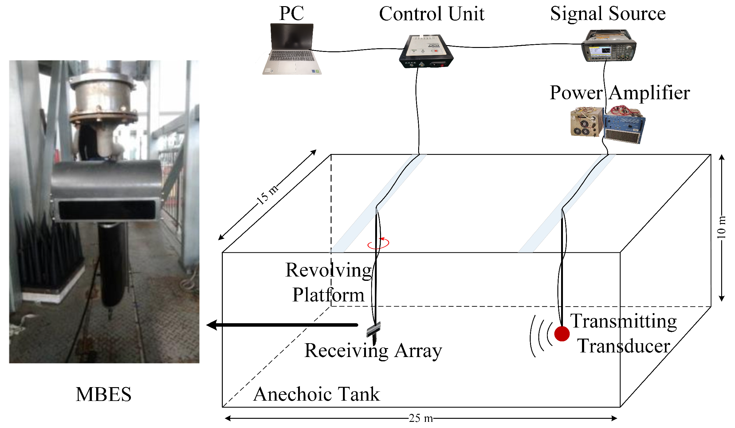
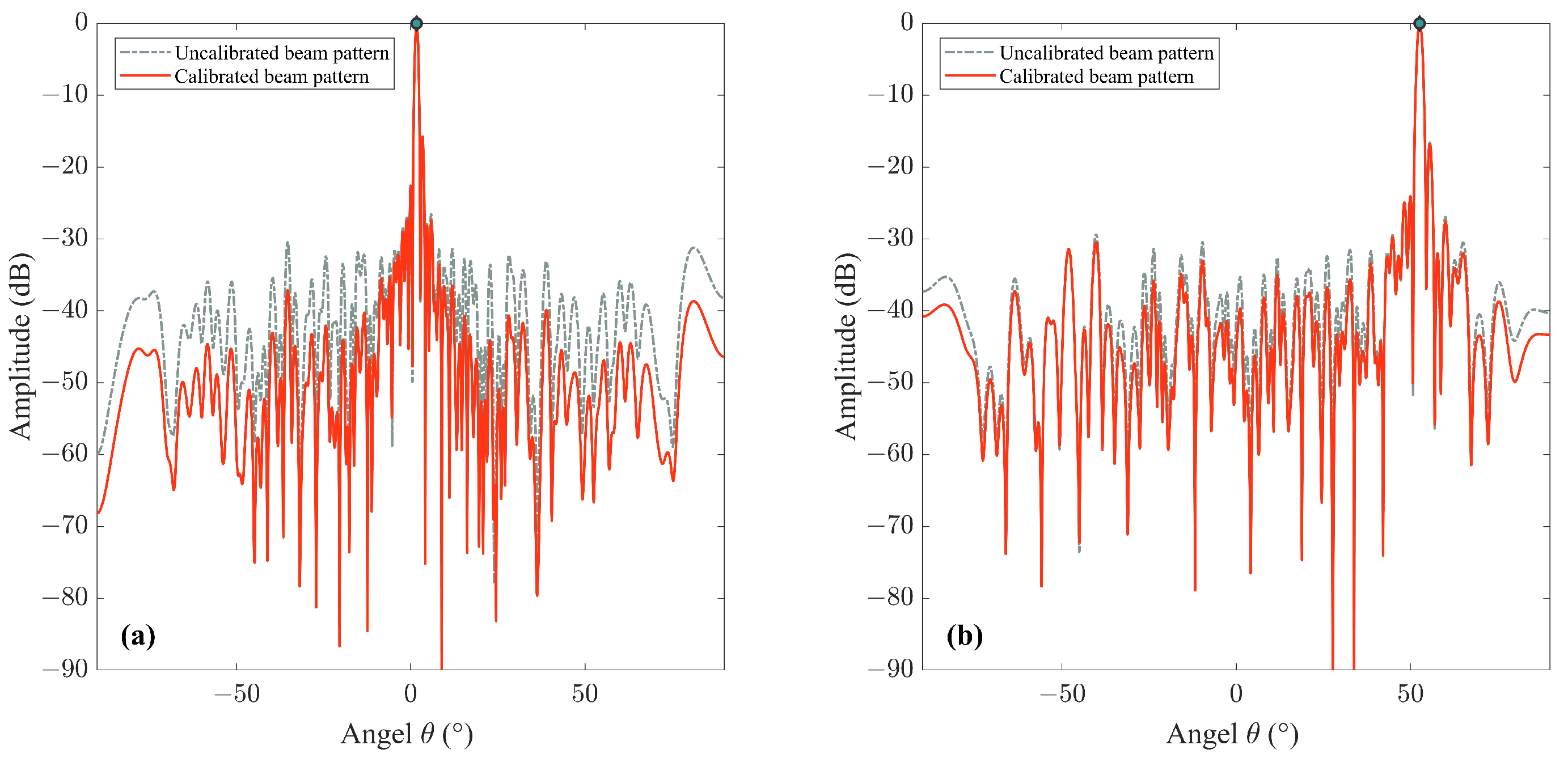
4.2. Tank Experiment

In this section, a tank experiment was conducted to correct mutual coupling of the receiving array of the MBES. The acoustic centers of the transmitting transducer and the receiving array were located at the same depth. This alignment mitigates mutual coupling effects. The near-field condition was satisfied in this experiment. This ensures accurate experimental conditions.

Figure 5 illustrates the layout diagram of the equipment and the receiving array targeted for correction. The experiment was conducted in an anechoic tank with dimensions of 25 m in length, 15 m in width, and 10 m in depth. An electrical signal with 0.1 ms pulse width is generated using a signal generator. Initially, the signal waveform is of low power; however, it is subsequently amplified by a signal amplifier to enhance its power. Finally, the electrical signal undergoes electric-acoustic conversion through a transmitting transducer to produce an acoustic signal. Meanwhile, the receiving array captures the acoustic signal and then transmit the data to the PC for processing through the control unit. The MBES control system must be used to accurately synchronize data acquisition and acoustic signal transmission during measurements where the rotary station rotates continuously. This ensures data integrity and alignment with the platform’s movement.

Table 3. The operational parameters of the devices in the tank experiment.

Parameters	Value	Parameters	Value
Signal frequency	200 kHz	Pulse width	0.1 ms
Sampling rate	85.356 kHz	Number of elements	100
Receiving distance	10 m	Element spacing	3.75 mm
Rotation rate	$0.6$°/s	Sound velocity	1486 m/s
Rotation accuracy	$0.1$°/s	Transmission interval	1 s

provides an overview of the operational parameters.

A dataset comprising 300 datasets with a $0.6$° angular interval was collected. For near-field focused beamforming, two distinct datasets with varying orientations were carefully chosen and subsequently calibrated using the procedures outlined in Table 1.

Following data collection, the processed data are presented in Figure 6, illustrating the results of beamforming at various angles. As depicted in the beam pattern, the discrepancy in DOA estimation accuracy before and after mutual coupling calibration is not pronounced. This is attributed to the MBES array consisting of 100 elements and achieving a high DOA estimation accuracy. The impact of mutual coupling calibration becomes more apparent with a lower array number or when employing multi-subarray technology and sparse array processing. Contrastingly, regarding sidelobe amplitude suppression, a conspicuous reduction in the sidelobe level of the beam pattern is evident post mutual coupling calibration compared to its pre-calibration state. Consequently, cross-coupling calibration significantly enhances robustness.

5. Discussion and Conclusions

This paper presents a correction method for addressing mutual coupling among array elements, utilizing focused beamforming techniques. The primary objective of this method is to enhance the accuracy of DOA estimation in the context of underwater acoustic transducers. Primarily, the near-field propagation model of ULA in MBES is analyzed and the mutual coupling effect is investigated. The calibration technique presented herein, which leverages the near-field focused beamforming technology, alleviates the limitations of the conventional approaches. Typically, such conventional methods do not impose size limitations on the test tank and are primarily tailored for arrays featuring a substantial number of elements. In addition, our approach allows the construction of the receiving signal’s covariance matrix using a single snapshot in the frequency domain, eliminating the need for a low-pass filtering step. During the calibration process, the Toeplitz property of the mutual coupling matrix is utilized to transform estimation outcomes into an independent format. Ultimately, a joint estimation of both DOA and mutual coupling coefficients is achieved. The efficacy of this algorithm is verified through simulation and tank experiments.

While the presented method is rooted in the amalgamation of well-established algorithms, it is implemented for sonar array calibration utilizing different strategies. This approach effectively addresses the problem of mutual coupling in the calibration of MBES arrays. In practical engineering scenarios, the mutual coupling effect among array elements, arising from deviations or perturbations in array manifolds, poses a challenge to the high-resolution spectral estimation algorithm. This issue can be efficiently addressed through the application of the proposed method. Moving forward, we aim to integrate signal theory from sonar heterogeneous arrays to substantiate the universality of this approach. Simultaneously, the method can be extended to analyze mutual coupling in sonar sparse arrays.

References

1. Rubio, S.S.; Romero, A.S.; Andreo, F.C.; Gallero, R.G.; Rengel, J.; Rioja, L.; Callejo, J.; Bethencourt, M. Comparison between the employment of a multibeam echosounder on an unmanned surface vehicle and traditional photogrammetry as techniques for documentation and monitoring of shallow-water cultural heritage sites: A case study in the bay of Algeciras. J. Mar. Sci. Eng. 2023, 11, 1339. [Google Scholar]
2. Zhang, W.; Zhou, T.; Li, J.; Xu, C. An efficient method for detection and quantitation of underwater gas leakage based on a 300-kHz multibeam sonar. Remote Sens. 2022, 14, 4301. [Google Scholar] [CrossRef]
3. Wang, J.; Li, H.; Huo, G.; Li, C.; Wei, Y. A multi-beam seafloor constant false alarm detection method based on weighted element averaging. J. Mar. Sci. Eng. 2023, 11, 513. [Google Scholar] [CrossRef]
4. Fascistam, A. Toward integrated large-scale environmental monitoring using WSN/UAV/Crowdsensing: A review of applications, signal processing, and future perspectives. Sensors 2022, 22, 1824. [Google Scholar] [CrossRef]
5. Habib, A.; Zhou, T.; Masjedi, A.; Zhang, Z.; Evan Flatt, J.; Crawford, M. Boresight calibration of GNSS/INS-Assisted push-broom hyperspectral scanners on UAV platforms. IEEE J. Sel. Top. Appl. Earth Obs. Remote Sens. 2018, 11, 1734–1749. [Google Scholar] [CrossRef]
6. Dai, J.; Zhao, D.; Ji, X. A sparse representation method for DOA estimation with unknown mutual coupling. IEEE Antennas Wirel. Propag. Lett. 2012, 11, 1210–1213. [Google Scholar] [CrossRef]
7. Zhang, J.; Qiu, T.; Luan, S. Robust Sparse Representation for DOA Estimation With Unknown Mutual Coupling Under Impulsive Noise. IEEE Commun. Lett. 2020, 24, 1455–1458. [Google Scholar] [CrossRef]
8. Guo, R.; Li, W.; Zhang, Y.; Chen, Z. New direction of arrival estimation of coherent signals based on reconstructing matrix under unknown mutual coupling. J. Appl. Remote. Sens. 2016, 10, 015013. [Google Scholar] [CrossRef]
9. Tang, W.; Jiang, H.; Zhang, Q. Off-Grid DOA estimation with mutual coupling via block log-sum minimization and iterative gradient descent. IEEE Wirel. Commun. Lett. 2022, 11, 343–347. [Google Scholar] [CrossRef]
10. Li, H.; Wei, P. DOA estimation in an antenna array with mutual coupling based on ESPRIT. In Proceedings of the International Workshop on Microwave and Millimeter Wave Circuits and System Technology, Chengdu, China, 24–25 October 2013; pp. 86–89. [Google Scholar]
11. Zhang, Q.; Li, J.; Li, Y.; Li, P. A DOA tracking method based on offset compensation using nested array. IEEE Trans. Circuits Syst. II Express Briefs 2021, 69, 1917–1921. [Google Scholar] [CrossRef]
12. Pulipati, S.; Arivarathna, V.; Perera, S.M.; Wijenayake, C.; Belostotski, L.; Madanayake, A. Digital uncoupling of coupled multi-beam arrays. In Proceedings of the International Applied Computational Electromagnetics Society Symposium (ACES), Hamilton, ON, Canada, 1–5 August 2021; pp. 1–4. [Google Scholar]
13. Liu, C.; Vaidyanathan, P.P. Super nested arrays: Linear sparse arrays with reduced mutual coupling—Part I: Fundamentals. IEEE Trans. Signal Process. 2016, 64, 3997–4012. [Google Scholar] [CrossRef]
14. Mei, F.; Xu, H.; Jian, C.; Zhang, J. A super transformed nested array with reduced mutual coupling for direction of arrival estimation of non-circular signals. IET Radar Sonar Navig. 2022, 16, 799–814. [Google Scholar] [CrossRef]
15. Friedlander, B.L.; Weiss, A.J. Direction finding in the presence of mutual coupling. IEEE Trans. Antennas Propag. 1991, 39, 273–284. [Google Scholar] [CrossRef]
16. Svantesson, T. Modeling and estimation of mutual coupling in a uniform linear array of dipoles. In Proceedings of the IEEE International Conference on Acoustics, Speech, and Signal Processing (ICASSP), Phoenix, AZ, USA, 15–19 March 1999; pp. 2961–2964. [Google Scholar]
17. Svantesson, T. Mutual coupling compensation using subspace fitting. In Proceedings of the IEEE Sensor Array and Multichannel Signal Processing Workshop (SAM), Cambridge, MA, USA, 17 March 2000; pp. 494–498. [Google Scholar]
18. Liao, B.; Zhang, Z.; Chan, S. DOA estimation and tracking of ULAs with mutual coupling. IEEE Trans. Aerosp. Electron. Syst. 2012, 48, 891–905. [Google Scholar] [CrossRef]
19. Hu, W.; Wang, Q. DOA estimation for UCA in the presence of mutual coupling via error model equivalence. IEEE Wirel. Commun. Lett. 2020, 9, 121–124. [Google Scholar] [CrossRef]
20. Yuan, W.; Zhou, T.; Shen, J.; Du, W.; Wei, B.; Wang, T. Correction method for magnitude and phase variations in acoustic arrays based on focused beamforming. IEEE Trans. Instrum. Meas. 2020, 69, 6058–6069. [Google Scholar] [CrossRef]
21. Zheng, Z.; Liu, K.; Wang, W.; Yang, Y.; Yang, J. Robust adaptive beamforming against mutual coupling based on mutual coupling coefficients estimation. IEEE Trans. Veh. Technol. 2017, 66, 9124–9133. [Google Scholar] [CrossRef]
22. Wang, Y.; Wang, L.; Xie, J.; Trinkle, M.; Ng, B. DOA estimation under mutual coupling of uniform linear arrays using sparse reconstruction. IEEE Wirel. Commun. Lett. 2019, 8, 1004–1007. [Google Scholar] [CrossRef]
23. Meng, D.; Wang, X.; Huang, M.; Yin, Y.; Shen, C.; Zhang, K. Reweighted nuclear norm minimisation for DOA estimation with unknown mutual coupling. Electron. Lett. 2019, 55, 346–347. [Google Scholar] [CrossRef]
24. Wang, X.; Meng, D.; Huang, M.; Wan, L. Reweighted regularized sparse recovery for DOA estimation with unknown mutual coupling. IEEE Commun. Lett. 2019, 23, 290–293. [Google Scholar] [CrossRef]
25. Licitra, G.; Artuso, F.; Bernardini, M.; Moro, A.; Fidecaro, F.; Fredianelli, L. Acoustic beamforming algorithms and their applications in environmental noise. Curr. Pollut. Rep. 2023, 9, 486–509. [Google Scholar] [CrossRef]
26. Haxter, S.; Herold, G.; Huang, X.; Humphreys, W.; Leclère, Q.; Malgoezar, A.; Michel, U.; Padois, T.; Pereira, A.; Picard, C.; et al. A review of acoustic imaging methods using phased microphone arrays. CEAS Aeronaut J. 2019, 10, 197–230. [Google Scholar]
27. Chiariotti, P.; Martarelli, M.; Castellini, P. Acoustic beamforming for noise source localization - reviews, methodology and applications. Mech. Syst. Signal Process. 2019, 120, 422–448. [Google Scholar] [CrossRef]
28. Sun, S.; Wang, T.; Yang, H.; Chu, F. Damage identification of wind turbine blades using an adaptive method for compressive beamforming based on the generalized minimax-concave penalty function. Renew. Energy 2021, 181, 59–70. [Google Scholar] [CrossRef]
29. Jiang, Y.; Xu, W.; Chen, L.; Pan, X. Near-field beamforming for a Multi-Beam Echo Sounder: Approximation and error analysis. In Proceedings of the OCEANS’10, Sydney, NSW, Australia, 24–27 May 2010; pp. 1–4. [Google Scholar]
30. Singh, P.R.; Wang, Y.; Charge, P. Near field targets localization using bistatic MIMO system with spherical wavefront based model. In Proceedings of the 25th European Signal Processing Conference (EUSIPCO), Kos, Greece, 28 August–2 September 2017; pp. 2408–2412. [Google Scholar]
31. Qi, C.; Chen, Z.; Zhang, Y.; Wang, Y. DOA estimation and self-calibration algorithm for multiple subarrays in the presence of mutual coupling. IEE Proc.-Radar Sonar Navig. 2006, 153, 333–337. [Google Scholar] [CrossRef]
Figure 1. Schematic diagram of ULA near-field focusing acoustic beamforming model.
Jmse 12 00125 g001
Figure 2. Comparison of near-field beamforming results. (a) Beamforming results with mutual coupling. (b) Beamforming results after mutual coupling correction.
Jmse 12 00125 g002
Figure 3. Beam pattern results at range r = 5 m with know and unknown mutual coupling and the proposed method.
Jmse 12 00125 g003
Figure 4. Performance of the proposed method. (a) Comparison of DOA estimation error using the proposed method and the CRB results. (b) The RMSE results of mutual coupling coefficient estimation.
Jmse 12 00125 g004
Figure 5. Equipment layout diagram in the anechoic tank and the receiving array of MBES to be corrected.
Jmse 12 00125 g005
Figure 6. Beam pattern results before and after correction. (a) The estimation results at r = 12.29 m and θ = 1.71 ° . (b) The estimation results at r = 12.29 m and θ = 52.60 °.
Jmse 12 00125 g006