Carbon Intensity Assessment of a Bulk Carrier Operating in Different Sea State Conditions

Abstract

This work uses the environmental contour line approach to estimate the long-term extremes of carbon emission generated by a bulk carrier operating in different sea state conditions, utilising short-term analyses of the ship propulsion energy efficiency as a function of hull resistance in calm water due to appendages, aerodynamic resistance, and added wave resistance, resulting in the required permanent delivered power and the one induced by the waves. The analysis accounts for the ship’s main characteristics, operational profile based on mission conditions, and wave climatic data. All sources of inherent uncertainties are accounted for through the variability in the 3 h extreme value in any sea state in the long term, and the inverse first-order reliability method (IFORM) is employed in predicting the extreme operational carbon intensity indicator (CII). This study develops proper wave scatter diagrams as a function of the route description. The CII measures the energy efficiency of the installed propulsion system, accounting for the ship’s operational characteristics, such as the annual fuel consumption with corresponding CO₂ factors, annual distance travelled, and capacity. The present study is limited to one operation route but can be extended to any other possible voyage or sea area. The estimated CII defined from the complete probabilistic characterisation of the sea state conditions conditional to the short-term maximum response is a rational approach that can be used for optimising the ship’s main characteristics, propulsion system, operational profile, and chosen route to achieve the best ship performance and energy efficiency.

1. Introduction

The daily challenges of making a voyage, maintenance on the ship, and monitoring fuel consumption and CO₂ emissions are issues that improve the performance of a ship. Each voyage allows for optimising speed and ensuring the ship is sailing in the best draft and trim condition that minimises fuel consumption.

Several operational factors can be enhanced to increase fuel efficiency. The ship’s speed significantly impacts fuel consumption in a third or fourth power order, depending on the ship’s characteristics. This means that to double the vessel’s speed, it is necessary to have at least eight times more power. Although the reduction is significant, one must consider the market conditions, as sailing at lower speeds can represent commercial losses. Concerning the real decrease in fuel consumption of the world fleet with the adoption of slow steaming, IMO [1] reduced the fuel consumption.

Voyage planning optimisation, accounting for weather routing, has been a practice for many years in achieving efficient, economical ship operation and reducing environmental pollution. The objective is to choose the most appropriate route, considering wind speed, wave conditions, currents expected during the trip, and the specific characteristics of each ship.

Currently, the operational efficiency of a vessel or fleet is an essential factor, both for economic and environmental issues. These issues are the most important because any decision making, whether in operation or maintenance, generates a capital cost such that the ship-owners must be assured of their recovery with the operational improvement of the vessel.

With a correct management methodology with a ship energy efficiency maintenance program, implementing the improvements with more significant earning potential, with a trained team and a monitoring system, a shipping company can significantly reduce its costs and emissions of pollutants and greenhouse gases.

The concept of the ecological ship starts at the design stage, goes through the construction, and is completed with the operation and recycling phases, that is, throughout the ship’s life cycle. Like this, the ship must be designed, built, operated, and recycled to not harm the environment and human health during its life cycle [2,3].

IMO takes two approaches to reduce CO₂ emissions from existing ships. The technical approach relates to the Energy Efficiency Existing Ship Index (EEXI) requirements. The EEXI is almost identical to the required EEDI for new ships as of 2023 [4]. The operational approach introduces a carbon intensity indicator (CII) [5].

The annual operational CII of each ship is determined by dividing the total amount of CO₂ emitted by the total amount of transportation work performed in a given calendar year. It is encouraged to utilise different definitions of the operational carbon intensity indicators, such as the Energy Efficiency Performance Indicator (EEPI), cbDIST (for passenger ships), and clDIST (for a ro-ro ship) for trial purposes.

The adoption of more stringent environmental control standards allows for reducing gas emissions. With a joint performance involving ship designers, engine suppliers, shipowners, and, mainly, the petroleum distillate industry, it will be possible to employ better-quality fuels for marine use and reduce emissions of harmful gases. While the reasoning behind using alternative fuels is known, the practical implementation and feasibility are unclear. The Zero-Carbon Fuel Monitor developed in [6] assesses the readiness of fuels for maritime use in general. According to this assessment, the Technology Readiness Level (TRL) for producing ammonia, methanol, and methane as alternative fuels is 5, 4, and 2, respectively. This means that technology is validated in the lab (TRL 4) or in the relevant environment (TRL 5).

Regarding operational measures, some are related to the maintenance program and others to travel planning [7]. Complying with the engine maintenance program according to the manufacturer’s specifications is essential to maintain efficiency. Regarding travel planning, some precautions can be taken to reduce fuel consumption and gas emissions.

The ports are also important in mitigating the contamination of gases close to the coast, including implementing land energy supply by evaluating costs, benefits, security, etc. [8].

The energy efficiency of ship operations is significantly impacted by environmental elements, such as wind speed, wind direction, waves, water speed, and water depth. Due to these factors’ time-varying nature and uncertainty, it is challenging to accurately determine the optimal speeds for different parts of a ship route using traditional static optimisation methods. This is particularly difficult when weather conditions frequently change along the length of the route.

The need to consider the actual sea conditions has been pointed out in [9]. It is concluded that without considering the ship’s behaviour in waves, achieving the desired reduction in GHG would not be possible, and even the level of emissions may increase.

The current sea conditions for a particular route can be determined using a scatter diagram based on the sea area subdivisions that have been crossed according to BMT [10]. Soon, a similar application will be launched to ensure the safe transportation of breakbulk cargo while reducing the cost of securing it on the ship [11].

Recently, the contour line approach [12,13,14] has been applied to identify the extreme governing actions with the limit state analysis employing the inverse first- and second-order reliability approaches, and this is the approach used in the present study.

Because ship energy efficiency has been of much interest in recent years, the present study discusses how to perform a ship energy efficiency analysis of a bulk carrier operating in different sea states as a function of the hull resistance in calm water, resistance due to appendages, aerodynamic resistance, and added wave resistance, resulting in the required permanent and variable delivered power. The analysis accounts for the ship’s main characteristics, operational profile, and wave climatic data. Several specifically developed wave scatter diagrams describe the route and ship’s operational profile. The operational carbon intensity indicator measures the impact on the CO2 emission generated by a bulk carrier ship.

The contour line approach is adopted for estimating the ship’s extreme energy efficiency, which includes several steps of calculation, like the operational profile and assembling a composite wave scatter diagram, ship resistance transfer function, delivered power transfer function, short-term distribution of delivered power, and ship energy efficiency analysis represented by the carbon intensity indicator.

The present study takes a significant step further in analysing the ship’s energy efficiency, which can be an excellent way to go ahead starting from what was already stated in [15,16] which is only a function of the primary and auxiliary engine power, deadweight, and service speed. However, the existing regulation established the minimum power of the total installed power. According to the Level 1 assessment defined in [17] for different types of ships, some adverse conditions’ threshold values of the significant wave height, peak wave period, and mean speed were set.

The present study takes a further step in the ship energy efficiency analysis accounting for any ship-specific operational profile, sea state conditions, and ship characteristics. Knowing the ship traffic intensity, the current approach can serve as a tool for identifying the air pollution concentration in the open sea and surrounding port areas. The emission concentration can be estimated based on a ship movement trajectory prediction of air pollution, considering the wind speed, horizontal and vertical dispersion parameters as a function of the geographical location of the ships, effective emission height, weather conditions, and speed of the analysed ships. The developed approach can significantly contribute to developing new Emission Control Areas (ECAs).

2. Operational Profile

The energy efficiency of a ship’s propulsion system is estimated using the ship’s operational profile. The operational profile includes the route of the ship voyage defined by the areas of operation and the percentage time spent in any individual area; the relative time spent in each mode of operation; and the average speed and time spent at each speed in any sea state or wave height.

These data are combined with a statistical description of the wave climate for already defined areas, identifying a complete ship’s “operational profile”.

The speed and sea state are assumed to be independent when an operational profile is developed. The time spent in port should also be included to construct the lifetime operational profile.

The wave climate experienced by ships varies considerably depending on the area of operation. Wave data are available for most parts of the world. British Maritime Technology [10] published a compilation of wave data.

Assuming stationarity over a short period (1~3 h), the sea elevation can be described as a stationary, relatively narrow-banded, Gaussian random process. In usual practice, the sea states are assumed to be characterised by a single peaked spectrum, modelled by the ISSC parametric of Pierson and Moskowitz [16]. The Pierson–Moskowitz spectrum is only for developed sea states, whereas the JONSWAP [18] spectrum is for developing seas and a double-peaked spectrum for mixed seas.

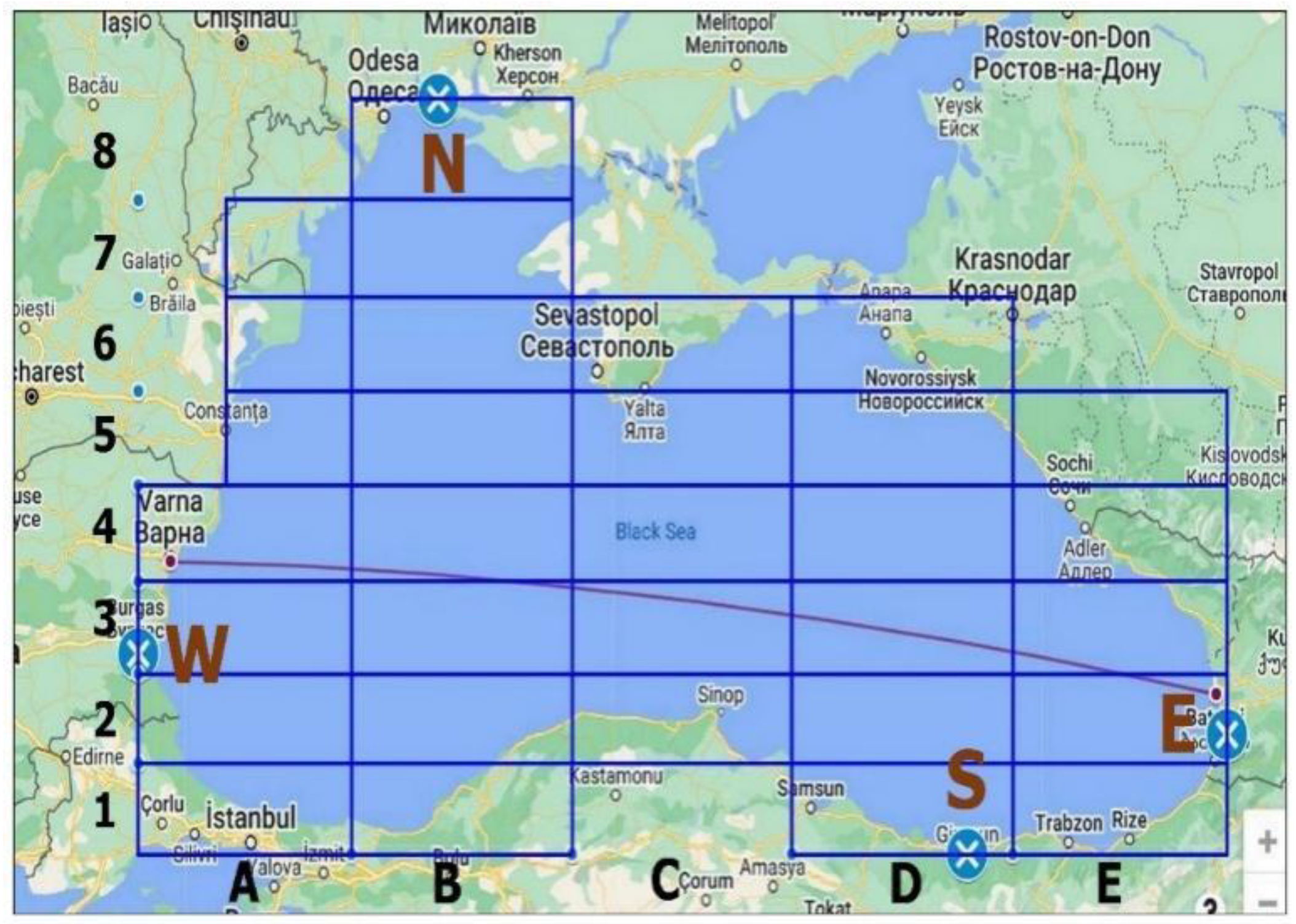
The sea surface of the Black Sea is divided into zones, each covering a geographic area over which the wave conditions are assumed uniform (Figure 1), where with N, W, S, and E, in red, are shown Nord, West, South and East (blue circles with a x in) and in black with A, B, C, D, E and 1, 2, 3, 4, 5, 6, 7 and 8 are identified any particular zone. The approximate dimensions of the rectangular zones are 237 × 79 (3:1) and consider the main traffic directions S-N and S -N-E., and vice versa.

The significant wave height and wave period data are extracted from the Copernicus Marine Service [19]. The Black Sea wave analysis and forecasts are generated using the WAM Cycle 6, a third-generation spectral wave model. The Black Sea version of the model is implemented on a spherical grid with a spatial resolution of approximately 2.5 km (1/40° × 1/40°) and includes 24 directional and 30 frequency bins. There are a total of 74,518 active wave model grid points in use. The length of the route analysed here, Varna–Poti–Varna, is 1234 nm. The route passes through zones A4, B4, C3, D3, E3, and E2 (see Figure 1).

The data collected are for 20 years, from 1 January 2002 to 31 December 2021. The observations are made every 3 h throughout the day, which makes a total of 2920 per year (2928 for a leap year). The total number of observations is 58,440.

The coordinates of the spherical grid in the crossed zones are presented in

Table 1. Geographical coordinates of the considered zones.

Zone	W	E	S	N
A4	27°30′0″	30°16′30″	43°02′60″	43°45′0″
B4	30°18′0″	33°10′30″	43°02′60″	43°45′0″
C3	33°12′0″	36°02′60″	42°21′0″	43°01′30″
D3	36°04′30″	38°57′0″	42°21′0″	43°01′30″
E3	38°58′30″	41°45′0″	42°21′0″	43°01′30″
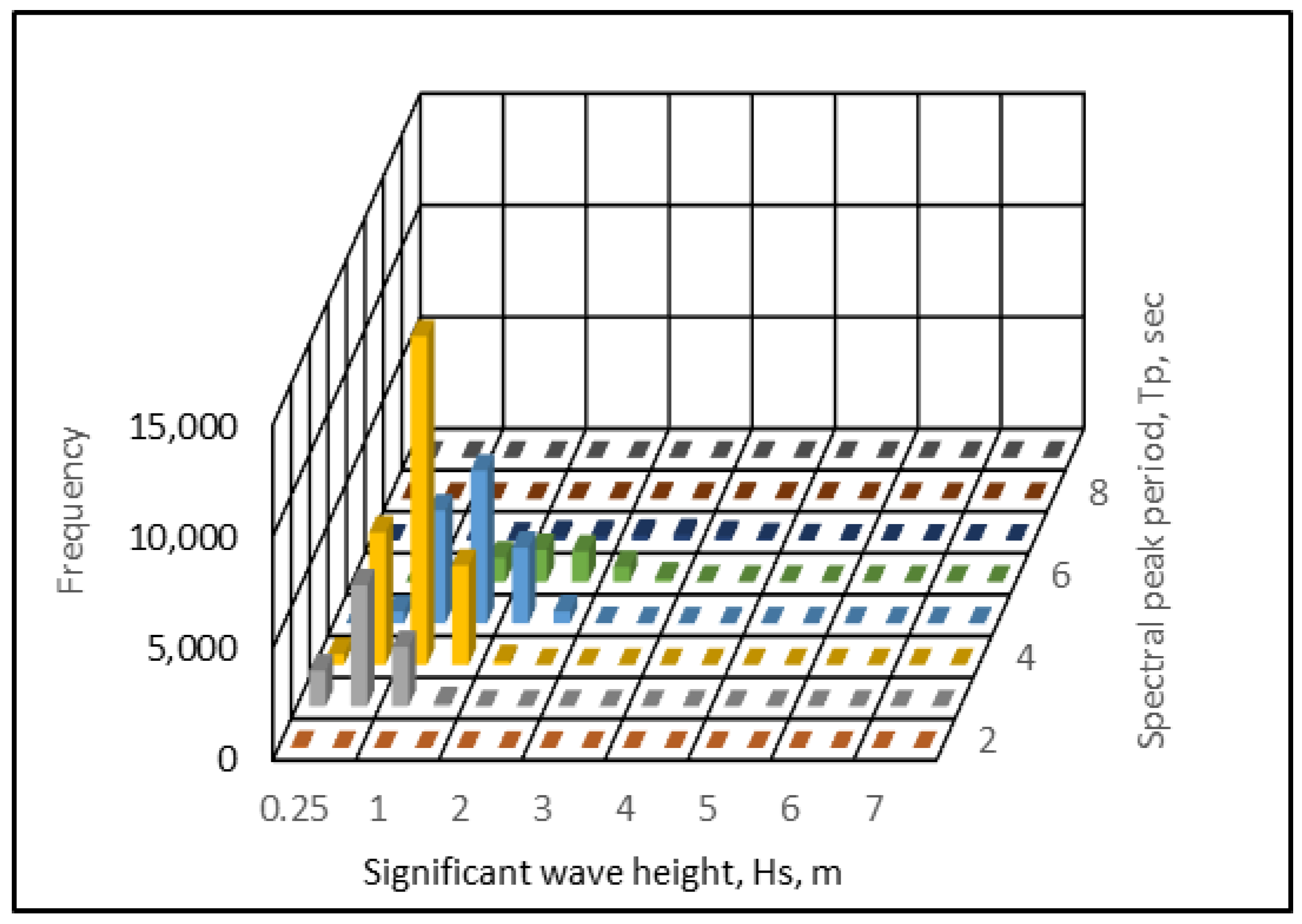
E2	38°58′30″	41°45′0″	41°37′30″	42°19′30″

, and the scatter diagram is in Figure 2, where the bars, in different colours, represent the frequency as a function of the significant wave height and spectral peak period

The long-term variability in the sea state characteristics defines the short-term sea state. The Weibull distribution [20] is used to determine the marginal distribution of the significant wave height $H_S$:

$$F_{H_S}=1-\mathrm{e}\mathrm{x}\mathrm{p}\left[-{\left(\frac{h-{\gamma }_{H_S}}{{\alpha }_{H_S}}\right)}^{{\beta }_{H_S}}\right]$$

(1)

where ${\alpha }_{H_S}$ is the scale parameter, ${\beta }_{H_S}$ is the shape parameter, and ${\gamma }_{H_S}$ is the location parameter. When ${\gamma }_{H_S}>0$, the observations below ${\gamma }_{H_S}$ are neglected. In the studied route of Varna–Poti, ${\alpha }_{H_S}=1.96$, ${\beta }_{H_S}$ = 1.25, and ${\gamma }_{H_S}$ = 0.5.

The zero-crossing wave period conditional on $H_S$ is modelled by a lognormal distribution:

$$f_{T_Z|H_S}=\frac{1}{{\sigma }_{T_p}t\sqrt{2\pi }}exp\left[-\frac{{\left(lnt-{\mu }_{T_P}\right)}^2}{2{\sigma }_{T_p}^2}\right]$$

(2)

where the distribution parameters ${\mu }_{T_P}\left(H_S\right)$ and ${\sigma }_{T_P}\left(H_S\right)$ are functions of the significant wave height $H_S$ [21]. A good fit to the observation data is given as:

$${\mu }_{T_P}\left(H_S\right)=a_0+a_1{H}_S^{a_2}$$

(3)

$${\sigma }_{T_P}\left(H_S\right)=b_0+b_1{e}^{b_2{H}_S}$$

(4)

where the coefficients $a_i,b_i,i=0, 1, 2$ are defined from the actual data from the Black Sea composite scatter diagram, including the sea zones as described in Equations (3) and (4), which are given in

Table 2. Descriptors of statistical characteristics.

	${\mathit{\mu }}_{{\mathit{T}}_{\mathit{P}}}\left({\mathit{H}}_{\mathit{S}}\right)$	${\mathit{\sigma }}_{{\mathit{T}}_{\mathit{P}}}\left({\mathit{H}}_{\mathit{S}}\right)$
$a_0,b_0$	1.26	0.01
$a_1,b_1$	0.32	0.21
$a_2,b_2$	0.58	−0.24

.

The distribution of the annual maximum significant wave height $H_{S,max}$ is defined as:

$$F_{H_{S,max,1yr}}\left(h\right)={F_{H_S}\left(h\right)}^n$$

(5)

where $n$ is the 3 h sea state in one year. The significant wave height with a return period $T_R$ is defined as

$$H_{S,T_R}={F_{H_S}}^{-1}\left(1-\frac{1}{n{T}_R}\right)$$

(6)

The environmental contour concept is used to define the extreme sea state condition [12], where the joint environmental model for $H_S,T_Z$ is defined as:

$$f_{H_S,T_P}\left(h,t\right)=f_{H_S}\left(h\right)f_{T_P|H_S}\left(t|h\right)$$

(7)

and the transformation to the standard normalised U-space leads to

$$\Phi \left(u_1\right)=F_{H_S}\left(h\right), \Phi \left(u_2\right)=F_{T_P|H_S}\left(t\right)$$

(8)

where

$$\sqrt{u_1^2+u_2^2}=\beta$$

(9)

where $\beta$ is the radius for the $n$-year contour.

The transformation of the circle into a contour in the environmental parameter space is made through:

$$H_S={F_{H_S}\left(\Phi \left(u_1\right)\right)}^{-1}{,T}_P={F_{{T_P|H}_S}\left(\Phi \left(u_2\right)\right)}^{-1}$$

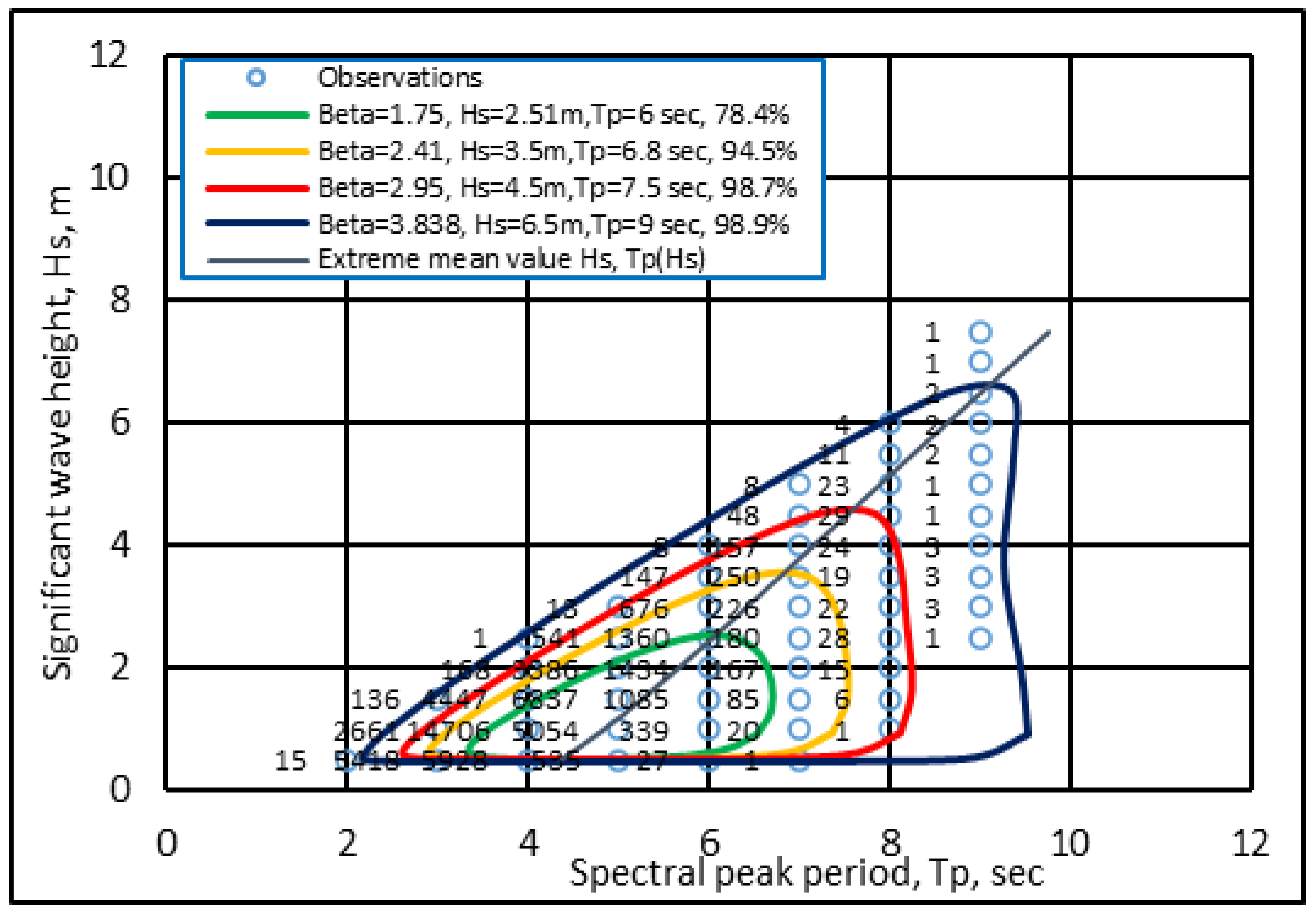
The Black Sea composite route contour in the environmental parameter space for $H_S$ = 2.5, 3.5, 4.5, and 6.5 m, including the observation frequency, can be seen in Figure 3.

The probability of a point being inside the contour of radius $\beta$ is given by:

$$P_{r,in}=\iint \Phi \left(u_1,u_2\right)d{u}_{1}d{u}_1=1-e^{-\frac{1}{2}{\beta }^2}$$

(10)

and the expected number of points inside the contour are defined as:

$$n_{in}=n_{a}Y\left(1-e^{-\frac{1}{2}{\beta }^2}\right)$$

(11)

where $n_a=$ 2928 is the annual average number of observations, and $Y=$ 20 yr is the year’s data covers; filtering a wave height less than 0.25 m leads to $n_{a}Y=\mathrm{56,266}$.

The main dimensions of the bulk carrier used in this study are given in

Table 3. Main dimensions of bulk carrier.

Length, $L_{pp}$, m	135.79
Beam, $B$, m	27.09
Depth, $D$, m	14.83
Draft, $T$, m	11.02
Block Coefficient, $C_B$	0.85
Ship Speed, $v_S$, knots	12
$DW$, tonne	30,291

.

The operational profile of the bulk carrier operating between Varna and Poti is shown in

Table 4. Operational profile.

Port 1	Varna–Poti	613 nm
Port 2	Poti–Varna	613 nm
Waiting time (round trip)	0.17	day
Navigation time (round trip)	4.26	day
Port loading capacity per day	115,200	tonne
Time for loading	2.17	day
Working days per year	360	day
Voyages/year	56
Ship cargo capacity	29,383	tonne
Annual cargo capacity	1,645,455	tonne

.

3. Transfer Function

The energy efficiency of a ship’s propulsion system is determined based on the ship resistance function, which is a function of the main characteristics of the ship, propeller, and ship’s operational profile, including matching the ship–engine–propeller by identifying the main and auxiliary engines and their specific consumptions.

The total ship resistance $R_T$ is defined as a sum of the frictional resistance $R_F$, the resistance due to the presence of the bulb $R_B$, the resistance of the immersed transom $R_{TR}$, the resistance due to appendages $R_A$, the aerodynamic resistance $R_{AIR}$, the model–ship correlation resistance $R_A$, and the added wave resistance $R_W$, and $k$ is the factor of the form:

$$R_T=R_F\left(1+k\right)+R_B+R_{TR}+R_{APP}+R_A+R_{AIR}+R_W$$

(12)

The resistance related to the calm weather, $R_P$:

$$R_P=R_F\left(1+k\right)+R_B+R_{TR}+R_{APP}+R_A$$

(13)

is defined based on the Holtrop and Mennes [22] approach and the aerodynamic resistance $R_{AIR}$ is based on the method presented in [23] A frequency response function for the wave-induced resistance $R_W\left(\omega {,v}_s\right)$ is used [24] where the total added wave-induced resistance is estimated as a sum of $R_{WR}\left(v_s\right)$, which is the added resistance due to the wave reflection and due to the motion effect $R_{WM}\left(\omega \right)$:

$$R_W\left(\omega {,v}_s\right)=R_{WR}\left(v_s\right)+R_{WM}\left(\omega \right)$$

(14)

$$R_{WR}\left(v_s\right)=\frac{2.25}{2}\rho gB{\varsigma }_a^2{\alpha }_T{sin}^{2}E\left(1+5\sqrt{\frac{L_{pp}}{\lambda }}{F}_n\right){\left(\frac{0.87}{C_B}\right)}^{1+4\sqrt{F_n}}$$

(15)

$$R_{WM}\left(\omega \right)=4\rho g{\varsigma }_a^2\frac{B^2}{L_{pp}}{\varpi }^{b_1}exp\left(\frac{b_1}{d_1}\left(1-{\varpi }^{d_1}\right)\right)a_1{a}_2$$

(16)

Kuroda, et.al. [25] identified that the corrective ${\alpha }_T$ draft coefficient is close to 1.0 for up to $\lambda /L=0.6$ and specific speeds. The average entrance angle $E$ is defined as:

$$E=atan\left(\frac{B}{2L_E}\right)$$

(17)

$$a_1=60.3C_B^{1.34}{\left(\frac{0.87}{C_B}\right)}^{1+F_n}$$

(18)

$$a_2=\left\{\begin{array}{c}0.0072+0.1676F_n\\ F_n^{1.5}exp\left(-3.5F_n\right)\end{array}\right.$$

(19)

The frequency of encounter $\varpi$ is given by:

$$\varpi =\left\{\begin{array}{c}\frac{\sqrt{\frac{L_{pp}}{g}}\sqrt[3]{\frac{k_{yy}}{L_{pp}}}{0.05}^{0.143}}{1.17}\omega , for F_n<0.05\\ \frac{\sqrt{\frac{L_{pp}}{g}}\sqrt[3]{\frac{k_{yy}}{L_{pp}}}{F_n}^{0.143}}{1.17}\omega , for{F}_n\ge 0.05\end{array}\right.$$

(20)

for $C_B\le 0.75:$

$$b_1=\left\{\begin{array}{c}11.0 for \varpi <1\\ -8.5 elsewhere\end{array}\right.$$

(21)

$$d_1=\left\{\begin{array}{c}14.0 for \varpi <1\\ -566{\left(\frac{L_{pp}}{B}\right)}^{-2.66}6 elsewhere\end{array}\right.$$

(22)

for $C_B>0.75$:

$$b_1=\left\{\begin{array}{c}11.0 for \varpi <1\\ -8.5 elsewhere\end{array}\right.$$

(23)

$$d_1=\left\{\begin{array}{c}566{\left(\frac{L_{pp}}{B}\right)}^{-2.66} for \varpi <1\\ -566{\left(\frac{L_{pp}}{B}\right)}^{-2.66}6 elsewhere\end{array}\right.$$

(24)

where ${\zeta }_a$ is the regular wave amplitude.

For the spectral analysis here, the total resistance $R_T$ is split into the one estimated for the calm sea conditions $R_P$ and added resistance due to wind $R_{CE}=R_{AIR}$, assumed as constant and wave-induced, defined as variable $R_{VE}$ = $R_W$:

$$R_T=R_P+R_{CE}+R_{VE}$$

(25)

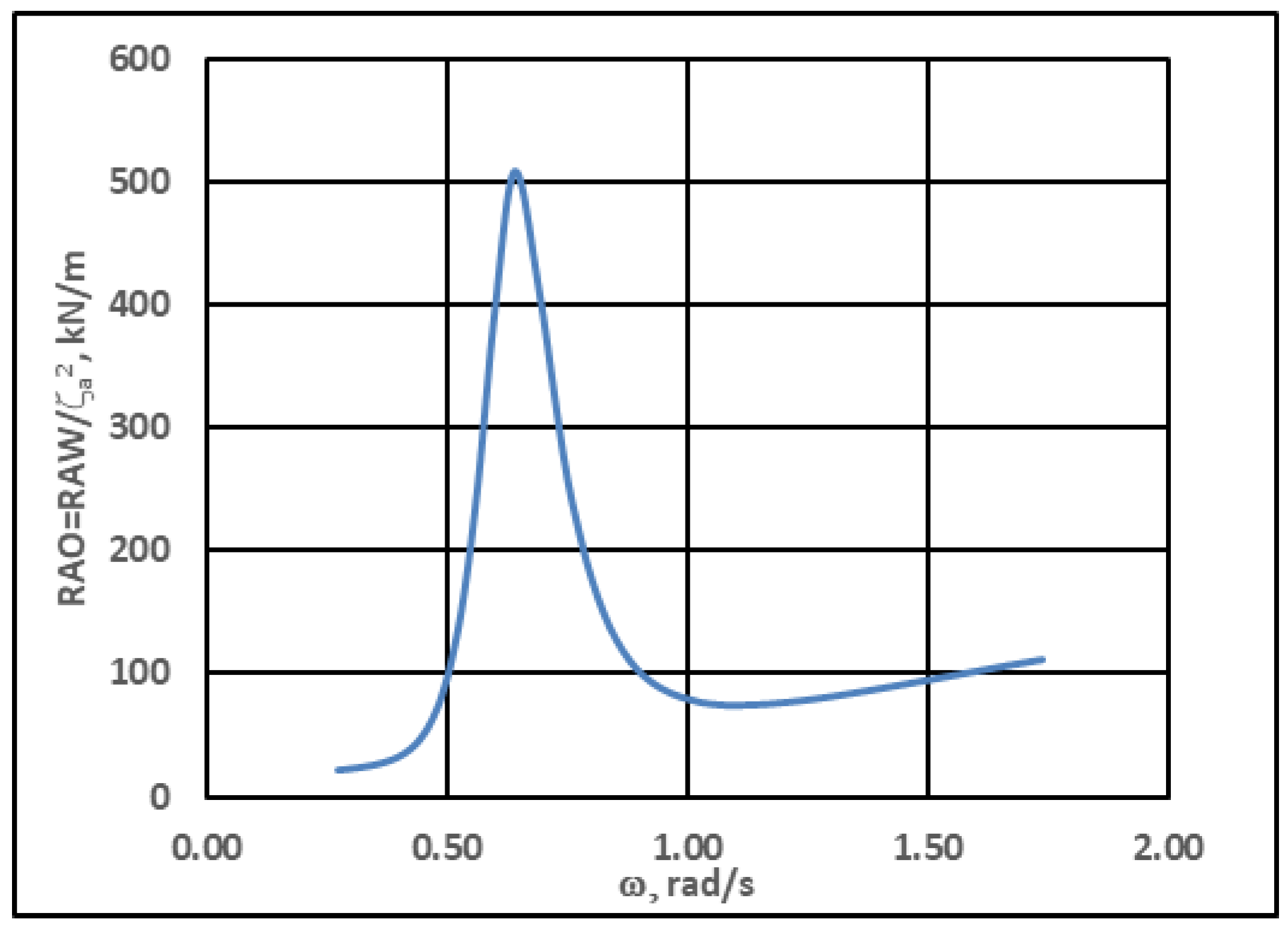
Wave-induced resistance for numerous conditions can be efficiently evaluated before estimating the ship’s energy efficiency based on the wave motion analysis of the response amplitude operators (RAOs). The RAOs define the amplitudes and phases in response to a wave of unit amplitude and a range of wave periods.

It is assumed that the wave-induced resistance response is linear as a function of the wave excitation. The total response in a seaway is a superposition of the responses to regular wave components constituting the irregular sea, which can be performed in the frequency domain. Given the linearity, the response is described by a stationary and ergodic but not necessarily a narrow-banded Gaussian process.

A numeric–empirical approach predicts wave-induced resistance effects. The transfer function is the basis of the wave-induced resistance response in the spectral analysis method. It represents the response of the wave-induced resistance as a function of a wave of a unit height.

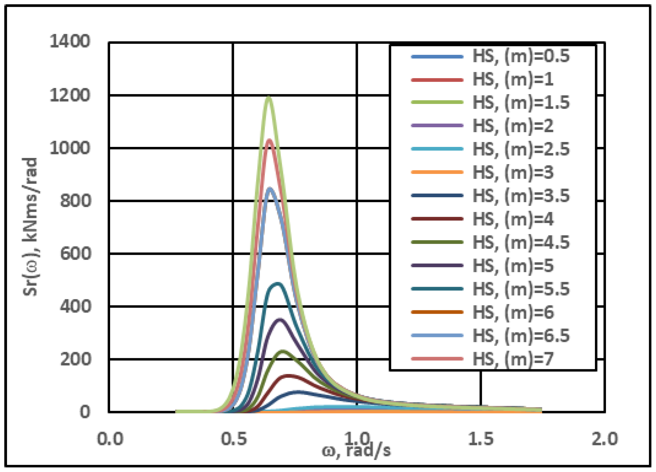
The wave-induced resistance RAO is developed, limited to the combination of speed and head sea and for every environmental condition represented by the scatter diagram, using the wave height and period as characteristic values with the sea spectrum. Each resulting wave-induced resistance response spectrum represents the short-term response to the operational profile and environmental conditions. The wave-induced resistance assessment is a long-term analysis that employs all data, where each response spectrum is multiplied by the probability of that combination. The result is a statistical distribution due to wave presence.

The nominal wave-induced resistance transfer function is defined based on parametric equations for the frequency response function:

$${{\Phi }_{VE}\left(\omega {,v}_S\right)}^2=\frac{R_{VE}\left(\omega {,v}_S\right)}{{\zeta }_a^2}$$

(26)

The primary source of the ship’s propeller power is the main engine producing brake power, $P_B$, which is transmitted to the delivered power $P_D$ of the propeller considering the transmission loss [26,27].

$$P_D=P_B{\eta }_{TRM}$$

(27)

where ${\eta }_{TRM}$ is the transmission efficiency. The delivered power acts on the propeller in the form of torque, $Q$:

$$P_D=2\pi nQ{\eta }_R$$

(28)

where ${\eta }_R$ is the relative rotation efficiency, and $n$ is the rotational speed.

The propeller’s efficiency factor ${\eta }_P$ depends on the shaft’s speed and rotational velocity.

The required advance coefficient of the propeller $T_{pr}$ is estimated from:

$$T_{pr}=\frac{{\rho }_w{u}_a^2{D}_p{K}_T\left(J\right)}{J^2}$$

(29)

where $D_p$ is the propeller diameter, $K_T\left(J\right)$ is the open-water propeller thrust coefficient, $J=u_a/\left(n{D}_p\right)$, and $u_a=u_s\left(1-w\right)$, and $J$ can be defined from the relationship of $K_T\left(J\right)/J^2$.

The required rotation rate of the propeller, $n_r$, in revolutions per second, is defined as:

$${n_r=u}_a/\left(J{D}_p\right)$$

(30)

The required delivered power to the propeller $P_{D,req}$ at the rotation rate $n_r$ is estimated as:

$$P_{D,req}=2\pi {\rho }_w{n}_r^3{D}_p^5{K}_Q\left(J\right)$$

(31)

where $K_Q\left(J\right)$ is the open-water propeller–torque coefficient curve, and the relative rotation efficiency is assumed to be close to 1.0.

The delivered power of the main engine is calculated as follows:

$$P_{D,P}=\frac{R_P+R_{CE}+R_{VE}}{{\eta }_0{\eta }_h}{v}_s$$

(32)

where ${\eta }_H$ is the hull efficiency and ${\eta }_o$ is the propeller efficiency in the open sea.

The main engine, propeller, and the engine limits given by the main engine manufacturer and propulsion system descriptors are shown in

Table 5. Propulsion system descriptors.

Description		Value
Propeller diameter, m	${\mathrm{D}}_{\mathrm{p}}^{}$	5.65
Number of blades	Z	3
Rotative efficiency	${\mathsf{\eta }}_{\mathrm{R}}$	1.02
Hull efficiency	${\mathsf{\eta }}_{\mathrm{H}}$	1
Shaft efficiency	${\mathsf{\eta }}_{\mathrm{S}}$	0.97
Propeller efficiency	${\mathsf{\eta }}_{\mathrm{P}}$	0.56
Main engine maximum power, kW	${\mathrm{P}}_{\mathrm{M}\mathrm{E}}$	4350
Main engine maximum rotation, rpm	${\mathrm{n}}_{\mathrm{M}\mathrm{E}}$	167
Specific fuel consumption, g/kWh	SFC	175
Main engine	ME	Wärtsilä

.

The main engine’s specific fuel consumption is 175 g/kWh for a 100% load, 156 g/kWh for 75%, and 166 g/kWh for a 50% load. The power required due to the electric balance is 976 kW, and the installed power is 1149 kW. Three auxiliary engines of 383 kW are installed, and the selected Genset is the MAN L16/24-5 cyl, 1000 rpm, with an SFC = 195 g/KWh.

4. Response Spectrum

The response spectrum of the wave-induced resistance based on the linear model is obtained directly from the wave spectrum and transfer function:

$$S_{VE}\left(\omega {,H}_S,T_P,v_S\right)={{\Phi }_{VE}\left(\omega {,v}_S\right)}^{2}S\left(\omega {,H}_S,T_P\right)$$

(33)

where ${{\Phi }_{VE}\left(\omega {,v}_S\right)}^2$ is the quadratic transfer function of the wave-induced resistance RAO, depending on an advanced speed, $v_S$, and wave frequency, $\omega$, and $S\left(\omega {,H}_S,T_P\right)$ is the wave JONSWAP spectrum [18].

Figure 4 shows the response amplitude operation spectrum, and Figure 5 shows the wave-induced resistance response amplitude operator.

The $n$th spectral moment of the response spectrum experienced on the wave-induced resistance is:

$$m_{VE,n}={\int }_0^{\mathrm{\infty }}{\omega }^n{S}_{VE}\left(\omega {,H}_S,T_P,v_S\right)d\omega$$

(34)

The zero moment of the delivered power $m_{P_D,0}$ is estimated as:

$$m_{P_{D,0,ijk}}=\frac{\left(R_P+R_{CE}+2m_{VE,0,i,j,k}\right)v_s}{2{\eta }_0{\eta }_h}$$

(35)

5. Response Statistics

From the estimated response spectrum of the wave-induced resistance, the peak distribution of the response in each stationary short-term period is determined using the response spectral moments. For a narrow-banded response process, the peaks are Rayleigh-distributed. In the case of the delivered power zero moment, the Rayleigh distribution of the delivered power is given [28] as:

$${F\left(P_D\right)}_i=1-exp\left(-\frac{{P_D}^2}{2m_{P_{D,i}}}\right),$$

(36)

where $m_{P_{D,0,i}}={\sigma }_{P_{D,i}}^2{m}_{P_{D,0,i}}$ is the zero-moment spectral moment. It must be pointed out that the distribution is conditional on $H_S$. For a narrow-banded process, the number of responses per second is approximated by:

$$n_i=\frac{1}{2\pi }\sqrt{\frac{m_{W,2,i}}{m_{W,0,i}}}$$

(37)

where $m_{W,2,ijk}$ is the second moment of the short-term response spectrum.

The total time is considered as many short intervals as possible, each of a few hours’ duration, during which the sea state remains constant. The ship’s lifetime probability density function of the peak values of the response ${\left[f\left(P_D\right)\right]}_L$ is presented as a weighted sum of the various short-term probability density functions to account for the relative frequency only limited to the variation in $H_S$, considering that $v_S$ is constant, and it is presented using the lifetime weighted sea method:

$${\left[f\left(P_D\right)\right]}_L=\frac{\sum _i{n}_{i}p{\left(H_s\right)}_i{\left[f\left(P_D\right)\right]}_i}{\sum _i{n}_{i}p{\left(H_s\right)}_i}$$

(38)

where ${\left[f\left(P_D\right)\right]}_i$ is the probability function for the peak values of the short-term response. The response for a given $H_S$ and $p{\left(H_S\right)}_i$ is the weighting factor for a sea state.

The Weibull distribution $F\left(P_D\right)$ can describe an adequate approximation for the long-term distribution of the delivered power and $Q\left(P_D\right)=1-F\left(P_D\right)$ is the probability of the exceedance of the delivered power, $P_D$, and $\beta =1.31$ and $\eta$ = 2775 are the Weibull shape and scale parameters.

The long-term delivered power response represents the most probable maximum, related to the extreme value distribution. There is a probability of exceeding the most probable maximum, and the expected value is associated with a 50% probability of being exceeded.

6. Ship Energy Efficiency

When evaluating a ship propulsion power system, it is essential to ensure that attained fuel consumptions are below the reference limit. Consumption may be classified as generated due to permanent, environmental, and variable actions. Permanent actions will not differ regarding magnitude over a specific period and are associated with resistance in calm weather. Wave-induced resistance relates to an environmental variable due to the change in magnitude from ordinary operations. The constant impact of the environment is related to air resistance. The relationship between the mean value fuel consumption (${\mu }_{FC}$), specific fuel consumption (SFC), and the delivered power (P) is defined as:

$${\mu }_{FC}={\int }_0^{t}PSFC\left(P\right)dt$$

(39)

The fuel consumption of ships depends on the vessel speed and the resistance developed from the ship during the voyage, and it is a function of the engine power, engine revolution per minute (RPM), vessel speed, sea state conditions, and vessel displacement. Furthermore, fuel consumption depends on the voyage type (laden or ballast) [29,30].

Once the expected delivery power is determined for the ship propulsion system in concern, the CII indicator calculations can be undertaken. The mean value fuel consumption ${\mu }_{FC}$ tonne/yr is estimated as:

$${\mu }_{FC}=\bullet \sum _1^2\sum _i^2{P_{i,j}SFC}_{i,j}{n}_j$$

(40)

where for a quay and sea operational condition, as given in Table 4, $n_1\approx 122$ days is the time spent in quay operation (calm) conditions, $n_2\approx 238$ days is the time spent in sea passage conditions, $i$ = 1 is related to the main engine, $i$ = 2 for the auxiliary engine, $j$ = 1 for sea conditions, and $j$ = 2 for calm conditions.

The ship operational characteristics considered for estimating the CII indicators are the ship design velocity, the specific fuel consumption, and the time spent in operation. The resulting fuel consumption, ${CO}_2$, and CII ratings are given in

Table 6. CII operational profile.

	Short Term, ${\mathit{H}}_{\mathit{S}}$ = 1 m	Short Term, ${\mathit{H}}_{\mathit{S}}$ = 2 m	Short Term, ${\mathit{H}}_{\mathit{S}}$ = 3 m	Short Term, ${\mathit{H}}_{\mathit{S}}$ = 4 m
FC, tonne/yr	3897	4029	4291	4775
${CO}_2$, tonne/yr	12,254	12,665	13,480	14,987
CII Rating	A	A	B	C

.

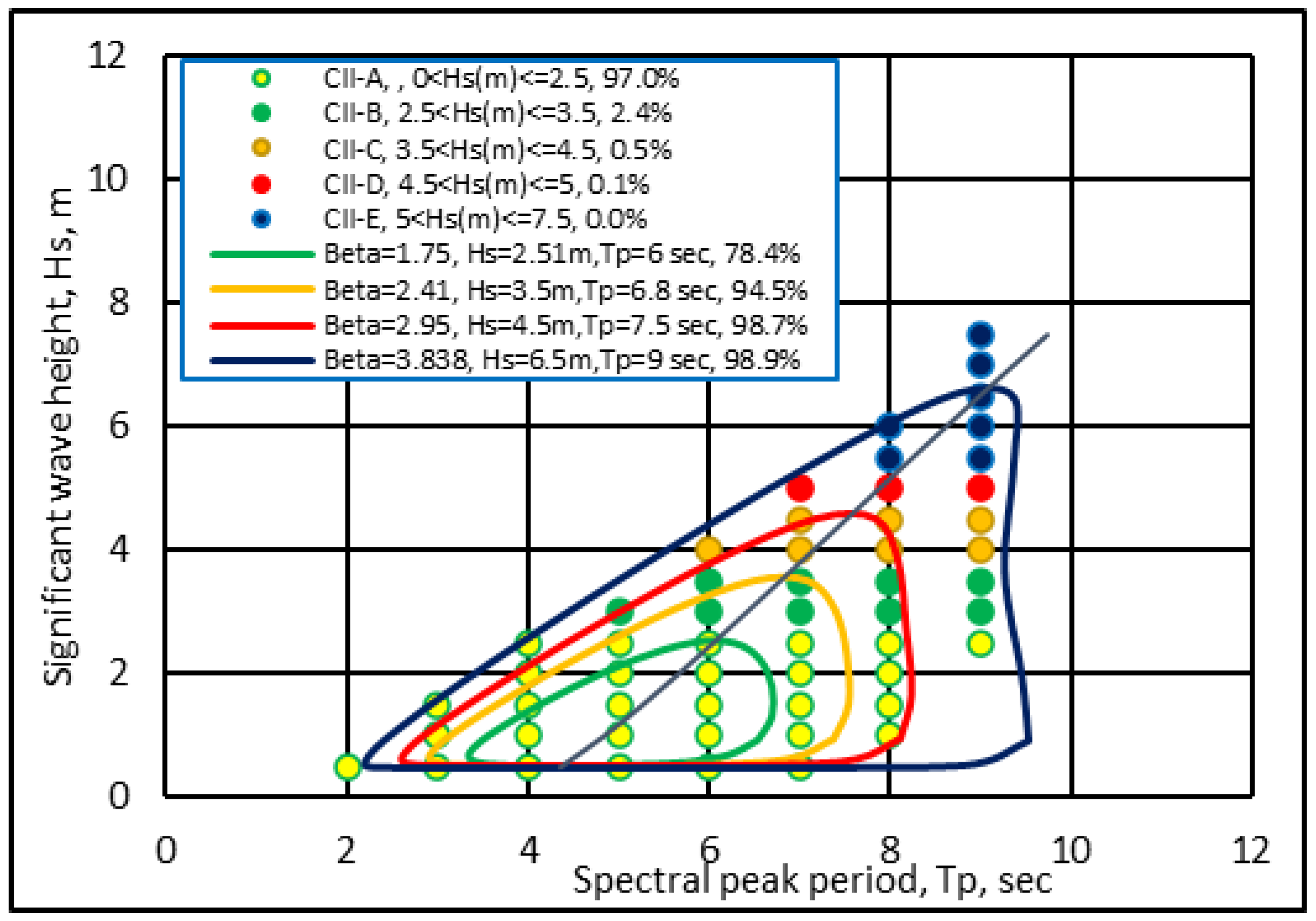
The environmental contour defines the extreme sea state condition, where the contour is a curve with equal probability corresponding to specific safety levels determined by a joint function of the significant wave height $H_S$ and the spectral peak period $T_P$.

The contour outlines the limit of safety, and if the sea state described by $H_S$ and $T_P$ is located inside the contour, then that sea state condition is acceptable. If not, then that sea state condition is an extreme condition causing unacceptable impact. The safety levels define extreme sea state conditions independently of the propulsion system design solution. The propulsion system behaves differently to extreme conditions, and extreme conditions vary (along the contour). Along the contour curve exists a point where the propulsion system response (delivered power) is the most significant and generates the most substantial CO₂ emissions. The maximum response depends on the propulsion system design, which is independent and placed on the same contour. Environmental contours define extreme sea state conditions in this regard, leading to extreme propulsion system responses [13].

The higher the wave is, the higher the wave-induced additional ship resistance, leading to higher delivered power. The wave period is also essential in locating the extreme wave height, and it is related to the ship’s propulsion dynamic response, represented by the response amplitude operator.

For any combination of $H_S$ and $T_P$, it results in different CO₂ quantities. The CII grades are shown in Figure 6. In 97% of all observed sea states, the generated CO₂ emissions belong to Class A, 2.4% to Class B, 0.5% to Class C, 0.1% to Class D, and less than 0.1% to Class E, respectively.

When evaluating the ship propulsion power system, it is essential to ensure that the attained CO₂ emissions are below the permissible emission reference limit defined in [5]. CO₂ emissions may be classified as generated due to permanent and variable environmental actions. Permanent actions will not differ regarding the magnitude over a specific period. Wave-induced resistance relates to an environmental variable action due to the change in magnitude from ordinary operations and the impact of the air resistance.

Regarding the ship and propulsion design criteria corresponding to a particular limit state, they are assumed to guarantee that no excessive ${CO}_2$ emissions are likely to occur during the intended operational lifetime of the ship. The requirement for ensuring clean transportation can be defined using the following limit state:

$${\gamma }_P{CO}_{2,P}+{\gamma }_V{CO}_{2,V}\le \frac{{CO}_{2,R}}{{\gamma }_R}$$

(41)

where ${CO}_{2,P}$ and ${CO}_{2,V}$ are the permanent and variable-generated ${CO}_2$ emissions; ${CO}_{2,R}$ is the characteristic reference limit emission as defined in, [5], and ${\gamma }_P$, ${\gamma }_V$, and ${\gamma }_R$ are partial safety factors to ensure a sufficient margin between the limit state ${CO}_2$ emission and the corresponding characteristic limit state response ${CO}_{2,R}$.

The detailed analysis performed here demonstrated that the observed sea states up to $H_S$ ≤ 2.5 m will generate ${CO}_2$ that belongs to the CII class A, class B relates to $H_S$ ≤ 3.5 m, class C relates to $H_S$ ≤ 4.5 m, class D relates to $H_S$ ≤ 5 m and class E relates to $H_S$ > 5 m.

A serviceability limit state (SLS) is the most suitable to ensure that fuel consumption does not interrupt the functionality of the normal operations of the ship propulsion system and that the ship emissions are below the characteristic limit state response as defined by the CII [3]. The characteristic quantities are expected to have a maximum value, and all safety factors are set to 1.0.

As can be noticed from Figure 6, the CII classes D (0.1%) and E (less than 0.1%) (blue and red dot) are sporadic events and, in the serviceability limit state, can be neglected. In this respect, accounting for the variability in the sea state, the extreme energy efficiency of the analysed bulk carried can be associated with the CII class C related to $H_S=4.5$ m and $T_P$ = 7.51 s and a beta index of 2.95 where the chosen sea state is a part of the contour line that covers 98.7% of all observed sea states.

The sea state descriptors are considered governing factors in defining the wave-induced resistance accounting for wave extremes and uncertainties in the ship propulsion system energy efficiency analysis. Uncertainties may cause the propulsion system to either be over-designed to achieve minimum CO₂ emissions or unsafe and generate over-emissions and environmental pollution. This trade-off is critical because the operator needs to invest as much as required to achieve the predefined safety level and zero GHGs in the coming years. Employing the formulation of contour lines for identifying the extremes of CO₂ emissions makes this study important in the energy efficiency analysis of any ship propulsion system.

However, the present study is limited to one operation route, but it can be extended to any other possible voyage or sea area. The actual route sea state conditions must be considered to optimise the ship’s main characteristics, propulsion system, and operational profile to achieve the best ship performance and energy efficiency. Any globalised general regulation may overdesign the ship’s main characteristics and propulsion system power capacity.

7. Conclusions

The contour line approach was employed to analyse the energy efficiency of a ship’s propulsion system operating in the Black Sea based on the detailed knowledge of the ship’s operational profile, including the projected route of the ship described in terms of the areas of operation and the percentage of time spent in these areas. The developed generic model can be used for any conventional commercial ship. The transfer function of the carbon intensity index in the short-term response was estimated using the frequency domain without prior measurements. The model employs empirical methods to define the calm water resistance, added resistance in waves, effective wake prediction, and thrust deduction, where the hull efficiency is estimated directly. The ship’s main characteristics, operational profile, and sea state conditions affect fuel consumption efficiency. The wave-induced resistance accounts for wave extremes and uncertainties in the energy efficiency analysis of the ship propulsion system. Employing the formulation of contour lines for identifying the extremes of CO₂ emissions makes this study important in the energy efficiency analysis of any ship propulsion system. It can be stressed that the results presented here are case-specific, which does not reduce the applicability of the method, which enables analysing and optimising the ship’s performance and energy efficiency operating in different sea state conditions. A comparative study was not performed with similar analysis or real measurements, which will be a future study of the present analysis. The present study takes a further step in the ship energy efficiency analysis accounting for any ship-specific operational profile, sea state conditions, and ship characteristics. Knowing the ship traffic intensity can be used to identify the air pollution concentration in the open sea and surrounding port areas. It can significantly contribute to developing new Emission Control Areas (ECAs).