Multi-Objective Optimization for Ship Scheduling with Port Congestion and Environmental Considerations

Abstract

Over the past several years, port congestion has become a severe problem, as ships are often not able to reach a series of ports based on the designed schedule, which induces changes in the schedules associated with port operations. Moreover, customers can not receive their cargo in a timely manner because of port congestion. This is not only an internal problem within the shipping industry but also calls for collaboration between shipping lines and their upstream or downstream members in the maritime supply chain, including shippers and port operators. This study concentrates on the tactical planning problem for optimizing ship schedules to determine the number of ships, the projected maximum speed, and the ship service schedule, which is set for a company on a certain route. We develop a novel multi-objective programming model for the green vessel scheduling problem under port congestion, and queuing theory is used to calculate the uncertain queuing times at ports. The ultimate goal of developing this model is to maximize cost efficiency, service reliability, and environmental benefits. A multi-objective grey wolf optimizer algorithm is introduced for solving this problem, which shows some computational advantages compared to the NSGA-II algorithm commonly used at the most advanced level. Experimental results verify the application of the model and confirm that more congested periods induce more service unreliability issues rather than additional costs and emissions generated. To this end, the proposed methodology would allow designing better liner shipping schedules to alleviate port congestion and provide sustainable shipping services.

1. Introduction

Over the past thirty years, as the fastest-growing category of the maritime industry, container shipping still maintains a good momentum [1,2]. Maritime transport carries more than 80 percent of the total merchandise trade in volume in the world, which bears the mainstay of worldwide integration and is located in the kernel part of cross-national transportation that sustains supply chains and facilitates international trade [3]. In the meantime, the surge in global trade volumes has unavoidably led to a rise in ships’ greenhouse gas (GHG) emissions. Among the seaborne trade volumes (including liquid bulk, bulk cargo, container, and normal cargo), 52% of carried goods in terms of value are transported through containerized vessels [4]. With the increasing maritime traffic volumes, more ship delays have occurred and caused disorder in port operational plans, which has further induced port congestion. In April of 2017, the Port of Shanghai suffered from severe port congestion issues, and the original schedules of 146 ships were seriously affected during this period, which can be explained by the main 10 liner shipping companies having restructured into 3 major alliances and undertaken extensive shipping route adjustments starting from 1 April. The situation at the port only became better in May. According to the 2015 Drewry report, some statistics showed that the average variance between the estimated time of arrival (ETA) and actual time of arrival (ATA) on three main Asia–Europe routes was 45.6 h in January and 50.4 h in February of 2015, respectively [5]. Many different sources of uncertainties may cause port delays and congestion, such as new shipping alliances (like the OCEAN alliance) which result in extensive shipping line adjustments, changes in port productivity, unexpected waiting time, or poor communication between marine terminal operators and shipping lines. Thus, there is a need for collaborative efforts from upstream to downstream stakeholders of maritime supply chains to optimize the shipping schedule and service efficiency.

Generally, the vessel scheduling problem involves fleet arrangement, schedule plans, speed choice, and routing design in a dynamic procedure, which signifies planning at both tactical and operational levels [6]. Various factors of liner shipping operations may lead to port congestion, such as increased ship delays, lower port operating efficiency, poor communication between marine terminal operators and shipping lines, and changes in the schedules of collaborating alliance partners. The uncertainties could be classified into two main categories [7]. One type refers to regular factors, e.g., port congestion (before berthing or before container handling), fluctuating terminal production rates, and accidental waiting time in the port channel [8]. Another type refers to rare incidents, e.g., poor weather and worker strikes [9]. According to Notteboom (2006) [8], port congestion (accidental waiting times before berthing or before starting handling) could account for 65.5%, the port production rate being lower than the standard expected could account for 20.6%, and the waiting time at anchorage for pilotage or towage could account for 4.7%. Clearly, over 90% of the schedule unreliability issues are related to port operations. A better contractual relation between shipping lines and ports would facilitate proper decisions and enhance service quality.

A lack of proper scheduling of terminal operations would lead to port congestion and uncertainties in vessel service at the port. Delayed vessel arrivals at the port have a negative influence on the seaside operations involving berth allocation, quay crane arrangement, container storage plan, and even cargo routing. Improper utilization of the available handling resources can cause ship delays and vice versa, e.g., container stacking and reshuffling operations [10] and berth and yard planning systems with low efficiency [11]. Waiting times and delays at ports put pressure on maritime supply chain stakeholders not only in terms of schedule reliability but also in terms of additional costs, including operational and fuel costs of the shipping line, container handling costs imposed on port operators, and cargo re-routing costs of shippers. Moreover, the vessel emissions produced by auxiliary engines during the port handling operations constitute a large portion of port pollutants, which will worsen the atmospheric environment and even threaten the daily life of people in the port vicinity.

To alleviate the negative impacts of port congestion, in this study, we allocate buffer times for each voyage leg according to the uncertain waiting times of vessels at ports, which are estimated by adopting the queuing methodology and calculated for each vessel queued at the anchorage point before the mooring period, which also fills the gap of modeling the implications of congested ports on the vessel schedule design. More specifically, a series of tactical planning decisions are addressed for designing effective vessel schedules. These decisions include the number of vessels for deployment, the queuing times, the sailing speeds, and the actual service schedule, considering the port congestion and arrival time windows. In this research, it is supposed that the shipping line acquires the port information in advance to enable tactical planning. Our goal is to realize the trade-offs between environmental, economic, and social objectives via multi-objective optimization. The applicability of the developed multi-objective mathematical model is tested by two metaheuristic approaches (i.e., the grey wolf optimizer algorithm and non-dominated sorting genetic algorithm II), which are able to generate Pareto optimal solutions for decision-makers in a timely manner. The computational performance of both algorithms is evaluated in detail.

The remaining portion of the paper is organized including the following parts. Section 2 gives a brief summary of the relevant literature. Section 3 constructs container shipping system dynamics (Section 3.1), discusses the applicability of queuing methodology (Section 3.2), and formulates a multi-objective optimization model to focus on port congestion and environmental issues (Section 3.3). Section 4 depicts two multi-objective metaheuristic algorithms adopted in this study to produce Pareto feasible solutions, while Section 5 demonstrates some computational experiments to validate the presented multi-objective optimization model and analyze the statistical results. Finally, Section 6 draws a conclusion by debating the major findings and trends along with the key future research directions.

2. Literature Review

Some relevant literature is summarized from content to methodology in four areas: the literature mentions operational strategies in liner shipping to alleviate uncertainties, utilizing the first-come-first-served (FCFS) rule for examining port terminal operations, cutting vessel emissions, and multiple sustainable objectives in the maritime industry.

Certain studies have investigated how the uncertainty at ports (such as uncertain waiting times, unexpected handling times, and so on) could be mitigated through tactical measures in liner shipping. Qi and Song (2012) [12] designed an optimal service schedule by assigning proper buffer times into the schedule to alleviate the uncertainties. The total expected fuel consumption and emissions were minimized within the speed constraints and different service levels. Wang and Meng (2012) [13] proposed a tactical-level liner ship route schedule problem by considering time uncertainties at sea and at ports, aiming to determine the arrival time of ships at each port of call, as well as the sailing speed within the transit time constraints. The authors come up with an exact cutting-plane-based solution algorithm, which was intended to solve the mixed-integer non-linear stochastic programming model. The validity of the model was demonstrated through numerical experiments. Wang and Meng (2012) [11] developed the above work by introducing the hedges against the uncertainties in terminal operations, which included the uncertain waiting time because of port congestion and the unexpected handling time. The robust model was designed for the recovery of vessel schedules by fast steaming. The presented mathematical model was solved by utilizing the sample average approximation approach, linearization technical skills, and a decomposition mode. The studies mentioned above regarding to vessel scheduling did not particularly apply the queuing methodology for modeling port congestion.

Container terminals that generally apply the FCFS rule to analyze the daily operating schedule for serving shipping lines are called multi-user terminals [14,15,16]. Some studies have applied queuing theory to minimize the waiting cost in the queuing system [17,18,19,20], while others have evaluated the efficiency or performance of ports by minimizing the waiting time [21,22,23,24]. Several studies have determined the best number of berths by reducing the total cost [25,26,27,28,29]. The present study will utilize queuing theory to calculate the waiting time of vessels entering ports, as a part of the port time used in the vessel scheduling problem.

Increased vessel emission has attracted the attention of shipping lines to environmental impacts along with the task of cutting environmental costs, which is a critical matter on the agenda of the International Maritime Organization (IMO). In accordance with the third IMO GHG (greenhouse gas) study [30], the total CO₂ emissions from the seaborne industry reached 796 million tonnes in 2012, which is expected to rise by 250% in 2050 with this growth rate. From the economic and environmental perspectives, various research studies have been performed on the vessel scheduling problem, reducing fuel consumption and CO₂ emissions [13,31]. In addition, some studies have captured the vessel CO₂ emissions generated in the port areas. For instance, Qi and Song (2012) [12] intended to minimize the total expected fuel consumption (and emissions) by considering uncertain port times. Tai and Lin (2013) [32] studied the emission reductions of air pollutants for global container shipping carriers utilizing slow steaming and daily service frequency strategies. The ship operations were categorized into three periods: berthing time, maneuvering, and at sea. Dulebenets (2018) [33] extended the cost objective to accommodate carbon emission costs at sea and ports. The experiments revealed that the design of vessel schedules would be substantially changed with various carbon dioxide taxation values, while the impact on port operations was found to be very limited.

Some extant literature has considered multiple objectives for sustainable developments in the shipping business. Mansouri et al. (2015) [34] examined environmental sustainability and the trade-offs of balancing economic and operational benefits by implementing multi-objective optimization as a decision support system to improve sustainability of maritime shipping. Cheng et al. (2015) [35] defined a ‘Sustainable maritime supply chain’, which intends to improve the competitiveness of the supply chain from customer satisfaction, social, and environmental requirements by integrating maritime organizational units and coordinating materials, information, and financial flows. To help in maintaining the sustainability of container shipping, port operations and vessel sailing voyages could be considered simultaneously. Dulebenets (2022) [31] studied multi-objective collaborative agreements between shipping lines and port terminal operators to assist with the selection of appropriate time windows for the arriving vessels and appropriate handling rates for their service. The proposed collaborative agreements incorporated the major economic and environmental perspectives. A novel multi-objective optimization approach stimulated by the goal programming and epsilon-constraint methods was proposed to resolve the issue.

Despite the fact that the aforementioned vessel scheduling studies captured the impacts of uncertainty at ports, the implications of congested ports on the vessel schedule design have not been analytically modeled. Therefore, we utilize queuing theory to predict the uncertain waiting times at ports before mooring. In addition, the queuing time of delayed vessels is used to address port congestion in vessel schedule design by allocating buffer times. Therefore, our novel mathematical model can be used to facilitate cooperation between shipping lines and port operators to provide vessel service. Due to the growing interest of shipping lines in environmental considerations, the overall carbon dioxide emissions are directly incorporated as well. Furthermore, to study the effects of multiple objectives, a multi-objective grey wolf optimizer (MOGWO) algorithm is introduced to resolve the developed optimization model and offer optimal or near-optimal solutions. The experimental results show that the introduced algorithm is better compared with the non-dominated sorting genetic algorithm II (NSGA-II), which is a popular multi-objective optimization algorithm.

3. Mathematical Formulation

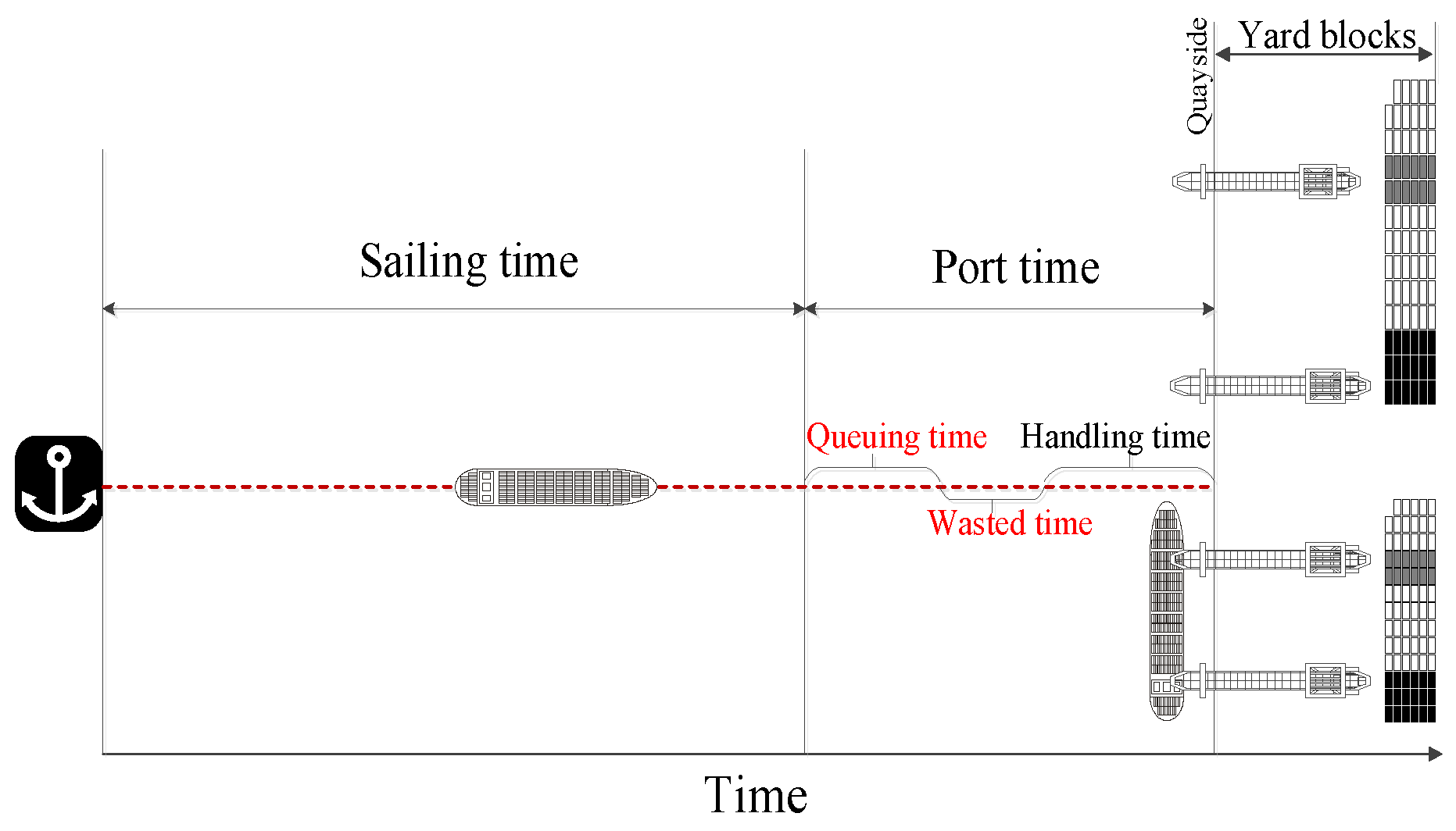
3.1. The System Dynamics

Liner service possesses the characteristics of regularity differing from other shipping sectors. A fleet of vessels call at a sequence of ports on a loop to provide a particular service frequency (normally weekly or bi-weekly), and they are operated by a global liner shipping company. From the practical perspective, the type of deployed ships, port rotation, and designed schedule on a shipping route is usually announced 3–6 months in advance. The whole voyage is separated into segments connecting each pair of contiguous ports, namely, the sailing cycle as the sum of transit time from each segment. However, small modifications to the service schedule, ship deployment, or port call sequence may still occur in case of disruptions.

According to Meng et al. (2014) [36], the decisions in containership routing and scheduling include three different planning levels: strategic, tactical, and operational levels. In this work, we concentrate on ship deployment, speed optimization, and schedule construction in tactical planning, with the assumption that the strategic level decisions (e.g., the service route, fleet size, and mix) are already given. Various uncertainties existing both at sea and at ports may induce vessels to deviate from the planned schedule, so ship delays have become a common phenomenon in recent years. Approximately 93.6% of ship delays are induced by port-related uncertainties (e.g., uncertain loading/unloading volume, congestion, mechanical breakdowns, availability of handling equipment) [8]. Based on the existing studies, the containerships are commonly assumed to arrive at a port following Poisson’s distribution [29,37]. We will utilize the queuing methodology to estimate the queuing time of containerships at congested ports. There are two different cases in practice when it comes to vessel queuing at ports. The first one uses the long-term cooperative agreements between ports and shipping liners applied to larger containerships, which determines the berthing location and yard allocation in advance. Ships arriving at the terminal will wait in a queue if the available berths are occupied, (i.e., the single server’s queuing law is applicable). The other case is to assign public berths randomly for ships, i.e., using the multi-server’s queuing law, which has also been used to obtain the optimal number of berths in some studies. Moreover, the extensive time wastage during the vessel arrival and departure processes cannot be neglected. The statistical analysis conducted by the Journal of Commerce (JOC) shows that up to USD 480 million could be acquired for 400,000 port calls made every year in the shipping industry if at least one hour of every port call could be eliminated and converted to slower sailing [38]. Therefore, liner shipping companies need to pay particular attention to the time spent at ports of call, rather than only focusing on the sailing time. During the execution stage, the vessel operator will not be able to travel any faster than the maximum speed to recover the delayed schedule. Moreover, a sailing speed increase may not be economically practical due to the rapid increase in fuel consumption at very high speeds, especially for larger container vessels [39].

This study models a typical liner ship route consisting of fixed ports of call based on Qi and Song (2012) [12], and each port can be called on more than once. It is assumed that homogeneous vessels would be arranged to retain weekly service frequency. Each port has a specific arrival time window, which varies for busy and idle ports. Hence, this study investigates the vessel scheduling problem with arrival time windows and transit time constraints deploying multiple vessels on one specific ship route. We will pay attention to the port time uncertainty and divide the whole voyage into the sailing periods and port periods, as depicted in Figure 1. This represents that the port period consists of queuing time at anchorage, wasted time (i.e., the time between the end of queuing time and the beginning of vessel handling time), and handling time. The type and number of arranged vessels, the service schedule, the transit times between ports, and the planned speed selection will be optimized herein.

Real data of vessel arrivals at one of the Shanghai Port terminals have verified that vessel arrivals follow the Poisson distribution (as discussed more in Section 5.1). Therefore, we assume that the arrivals of containerships calling at each port follow the Poisson distribution, and the multi-server FCFS law is applied for vessel service; here, vessels in this article refer particularly to containerships. Then, the queuing methodology can be used to calculate the waiting time of containerships in a queue. The other assumptions that will be further used in this study are summarized below:

• The same type of vessel is deployed on the given liner route with a fixed sequence of ports of call, and all vessels are chartered;
• Even if any service schedule on these ship routes is adjusted, all vessels still arrive randomly following the Poisson distribution;
• If the berthing positions of vessels are known in advance, the single server queuing law ($M/M/1$) will be applied to calculate the waiting times. However, if the berthing positions are not yet known, the multi-server queuing law ($M/M/c$) will be applied;
• The loading and unloading volume at each port is assumed to be constant (i.e., the total amount of import containers unloaded from vessels and the total amount of export containers loaded on vessels are assumed to be fixed);
• If a vessel arrives at a port earlier than the planned arrival time, it will be required to wait for handling until the planned arrival time starts [39,40];
• The speed on each leg can be changed and optimized in the range between the minimum speed and the planned maximum speed. However, the use of higher vessel sailing speeds will cause higher fuel consumption.

Before formally describing the proposed model formulation, we introduce the notation in the Abbreviation part.

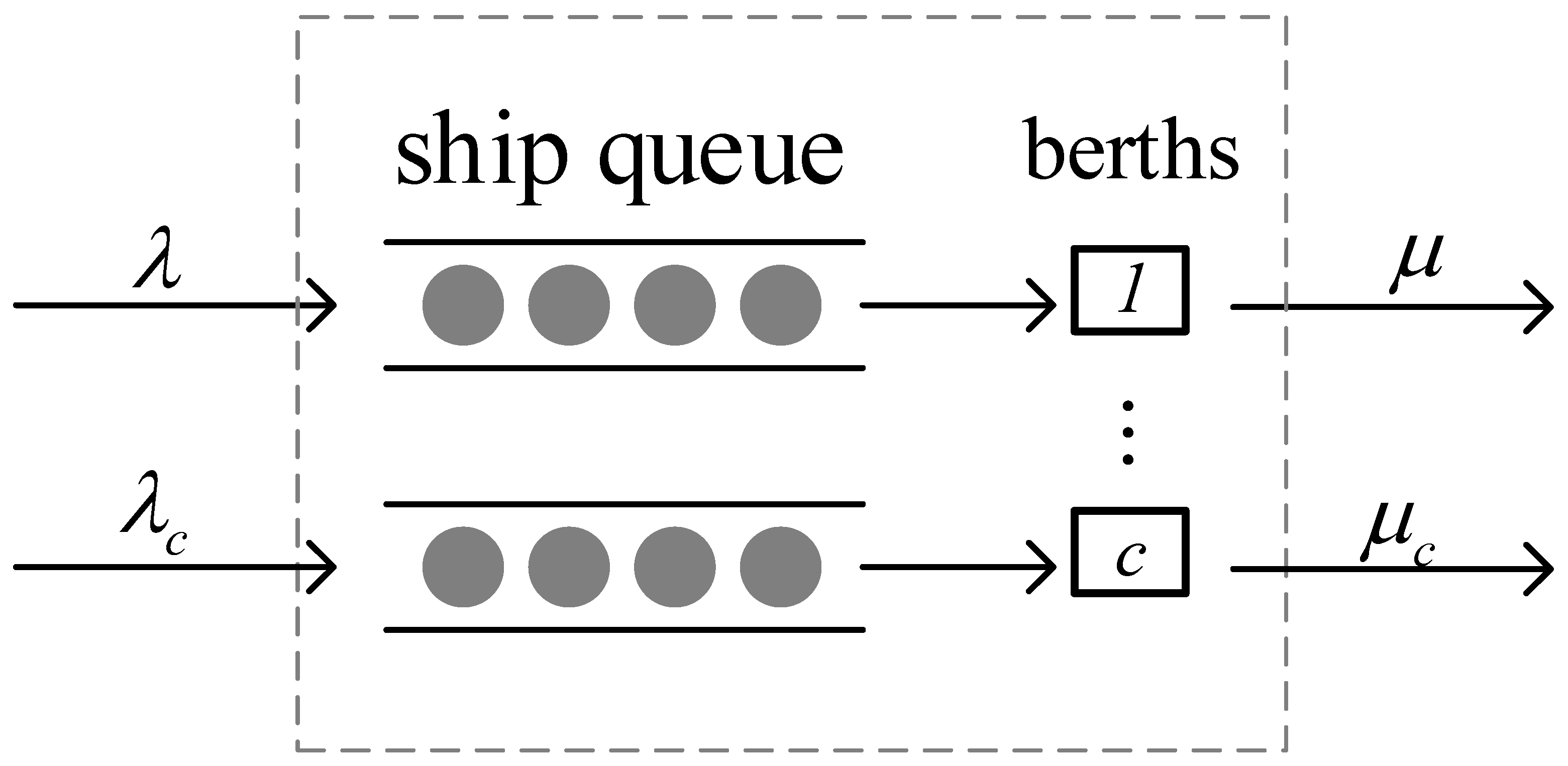
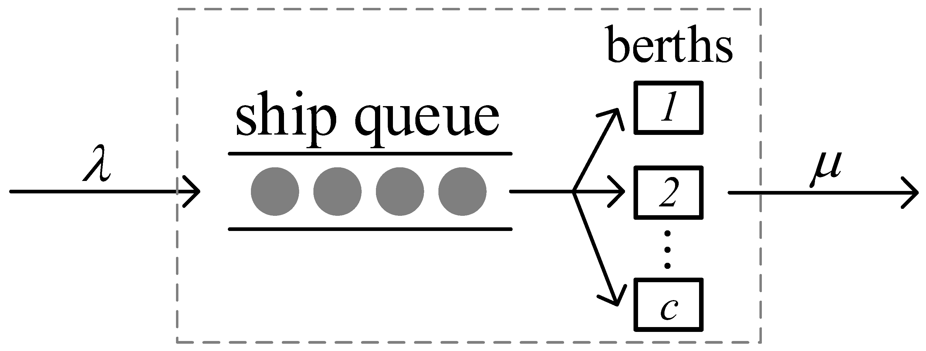
3.2. Queuing Time at Single-Berth and Multi-Berth Facilities

Queuing theory, as a branch of operational research, is generally used to calculate waiting time in lines or queues [41]. Previous studies that have applied queuing theory in maritime shipping often focused on assessing port performance, estimating the best number of berths or addressing the congestion issues. As Jansson and Shneerson (1982) [37] declared, ships often arrive at a port randomly and mostly follow Poisson’s distribution. During the berthing process, ships arrive at a port and need to wait at the anchorage point for the available berths to receive a container handling service, where ships and berths can be regarded as customers and servers, respectively. As mentioned above, one approach is to apply the $M/M/1$ queuing system in $c$ queues if ships have fixed (or pre-assigned) berthing positions, as shown in Figure 2. The other approach is to apply the $M/M/c$ queuing system for assigning ships to the available berths at random, as shown in Figure 3. The following assumptions were adopted for the queuing process:

(a)

The arrival process—ships arrive at random, subject to a Poisson probability distribution, and wait at the same anchorage point, even if vessel types can be different;

(b)

The queuing discipline—one waiting line and a ‘first-come-first-served’ rule. The arriving ships will wait when the berthing system is busy, and the queue length has an upper restriction;

(c)

The server discipline—each berth is mutually independent and has the same service ratio for the same type of ships. The service time is set as a random variable, subject to the negative exponential probability distribution.

• $M/M/1$ queuing system

The same type of vessels will wait in a queue at the anchorage point for the same berth. The expected number of ship arrivals at berth $c$ is ${\lambda }_c$, and the mean service rate at berth $c$ is ${\mu }_c$. The largest number of vessels that the queue accommodates is $X$, and the queue limit at each berth $c$ is $X_c$. According to the $M/M/1/N/\infty$ queuing theory, the mean occupancy rate is $\rho =\lambda /\mu$, while the other variables can be calculated in the following manner [42].

The probability that no ship will be served at berth $P_0$, and the probability that $n$ ships will be served at berth $P_n$, can be obtained from the following relationships:

$$P_0=\frac{1-\rho }{1-{\rho }^{N+1}}\rho \ne 1$$

(1)

$$P_n=\frac{1-\rho }{1-{\rho }^{N+1}}{\rho }^n\rho \ne 1,n\le X$$

(2)

The mean queuing length $L_c$ and the mean queuing time $q_c$ at berth $c$ can be calculated as follows:

$$L_c=\sum _{n=1}^{X_c}\left(n-1\right)P_n=\frac{\rho }{1-\rho }-\frac{\left(X_c+1\right){\rho }^{X_c+1}}{1-{\rho }^{X_c+1}}-\left(1-P_0\right)\rho \ne 1$$

(3)

$$q_c=\frac{L_c+\left(1-P_0\right)}{{\mu }_c\left(1-P_0\right)}-\frac{1}{{\mu }_c}\rho \ne 1$$

(4)

2.

$M/M/c$ queuing system

Since the different types of ships arrive and wait at the same anchorage point, the expected arrival rate $\lambda$ (ships/day) (the mean arrival interval between two ships—$1/\lambda$) is constant for all the ships. As shown in Figure 3, given the mean queue service rate of ships at berth $\mu$ (the mean service time per ship—$u=1/\mu$), the number of berths $c$, and the mean occupancy rate $\rho \left(\lambda /c\mu \right)$, the $M/M/c$ queuing system can be applied.

First, the mean service time per ship at each port of call (in days), i.e., the weighted average service time for all the ships, can be calculated using the subsequent equation:

$$u=\sum _v{u}_v{\lambda }_v/\sum _v{\lambda }_v$$

(5)

where $u_v$ is the mean service time of ship-type $v$, and ${\lambda }_v$ is the arrival number of ship-type $v$.

Then, according to Jansson and Shneerson (1982) [37], the probability of no ships arriving $P_0$ and the probability $P_n$ that $n$ ships arrive for service per day can be expressed using Equations (6) and (7) and considering the service intensity $\rho <1$:

$$P_0={\left[\sum _{n=0}^{c-1}\frac{1}{n!}{\left(\frac{\lambda }{\mu }\right)}^n+\frac{1}{c!}\cdot \frac{1}{1-\rho }\cdot {\left(\frac{\lambda }{\mu }\right)}^c\right]}^{-1}$$

(6)

$$P_n=\left\{\begin{array}{c}\frac{1}{n!}{\left(\frac{\lambda }{\mu }\right)}^n{P}_0\left(n\le c\right)\\ \frac{1}{c!c^{n-c}}{\left(\frac{\lambda }{\mu }\right)}^n{P}_0\left(n>c\right)\end{array}\right.$$

(7)

Furthermore, let $p=P_n\left(n\ge c\right)$ be the probability that a delay will occur, namely, there will be a delay when $n$ ships arrive at a port with $c$ berths, where $n\ge c$. Then, $p$ can be computed as follows:

$$p=\sum _{n=c}^{\infty }{P}_n=\frac{1}{c!\left(1-\rho \right)}{\left(\frac{\lambda }{\mu }\right)}^c{P}_0$$

(8)

Hence, the multi-berth queuing time $q$ can be calculated using Equation (9) while $\rho <1$ (Jansson and Shneerson, 1982):

$$q=\frac{u}{c\left(1-\rho \right)}\cdot p$$

(9)

However, when the service intensity is larger than 1 ($\rho >1$), we will limit the capacity of the queuing system to avoid the infinite queue of vessels waiting at the anchorage point. Then, the queuing time can be computed as follows [42].

The probability that no ship will be served at berth $P_0$ can be computed using the next equation:

$$P_0=\frac{1}{{\sum }_{k=0}^c\frac{{\left(c\rho \right)}^k}{k!}+\frac{c^c}{c!}\cdot \frac{\rho \left({\rho }^c-{\rho }^X\right)}{1-\rho }}\rho \ne 1$$

(10)

where $X$ represents the largest number of vessels allowed in the queuing system containing the vessels at berth and waiting at anchorage.

The probability that $X$ ships are in the terminal system (i.e., the system is full) can be computed using the next equation:

$$P_X=\frac{c^c}{c!}{\rho }^X{P}_0$$

(11)

The mean queuing length $L$ can be computed using the next equation:

$$L=\frac{P_0\rho {\left(c\rho \right)}^c}{c!{\left(1-\rho \right)}^2}\left[1-{\rho }^{X-c}-\left(X-c\right){\rho }^{X-c}\left(1-\rho \right)\right]$$

(12)

The mean queuing time $q$ can be computed using the next equation:

$$q=\frac{L}{\lambda \left(1-P_X\right)}$$

(13)

3.3. Multi-Objective Modeling

Not only in academic studies, but also at the execution stage of shipping operations, slow steaming has developed to become a popular and mature experience, both economically and environmentally beneficial. However, slow steaming may cause ship delays and late arrivals at consecutive ports of call. Considering port congestion, we formulate the green vessel scheduling model that aims to determine sailing speeds and service schedules by minimizing the annual total costs and carbon emissions, meanwhile minimizing the schedule unreliability as well.

$$\begin{gathered} Min{M}_{COST}=n_v·\left[\frac{C_{ho}}{K}\sum _{k=1}^K\sum _{i=1}^N{d}_i·g\left(s_{i,k}\right)+\frac{1}{K}\sum _{k=1}^K\sum _{i=1}^N\left[q_{i,k}\left(F_v^{ho}{C}_{ho}+F_v^{do}{C}_{do}\right)+\frac{\left(\omega +l_i\right)F_v^{do}{C}_{do}}{24}\right]\right] \\ ·\frac{365}{T/24}+n_v·C_v·365\left[C_{ho}\sum _{k=1}^K\sum _{i=1}^N{d}_i·g\left(s_{i,k}\right)+\sum _{k=1}^K\sum _{i=1}^N\left[q_{i,k}\left(F_v^{ho}{C}_{ho}+F_v^{do}{C}_{do}\right)+\frac{\left(\omega +l_i\right)F_v^{do}{C}_{do}}{24}\right]\right] \end{gathered}$$

$$·\frac{365}{7K}+n_v·C_v·365$$

(14)

$$Min{M}_{{CO}_2}=\gamma ·n_v·\frac{365}{T/24}·\left[\frac{1}{K}\sum _{k=1}^K\sum _{i=1}^N{d}_i·g\left(s_{i,k}\right)+\frac{1}{K}·\sum _{k=1}^K\sum _{i=1}^N\left[q_{i,k}\left(F_v^{ho}+F_v^{do}\right)+\frac{\left(\omega +l_i\right)F_v^{do}}{24}\right]\right]$$

$$\gamma ·\left[\sum _{k=1}^K\sum _{i=1}^N{d}_i·g\left(s_{i,k}\right)+\sum _{k=1}^K\sum _{i=1}^N\left[q_{i,k}\left(F_v^{ho}+F_v^{do}\right)+\frac{\left(\omega +l_i\right)F_v^{do}}{24}\right]\right]·\frac{365}{7K}$$

(15)

$$Min{M}_{SU}=\frac{1}{K·N}\sum _{k=1}^K\sum _{i=1}^{N}I\left\{t_{i,k}^a>t_{i,k}+W_i\right\}$$

(16)

First, we introduce the annual total cost minimization objective $M_{COST}$. As liner shipping is a capital-intensive industry, shipping lines pursue cost efficiency as their main goal, which consists of the fuel consumption cost during both the sailing period and port period, and the annual operating cost of all the vessels arranged on the route. Here, the operational cost refers to the charter hire for time-chartered ships.

Note that the component $\frac{1}{K}{\sum }_{k=1}^K{\sum }_{i=1}^N{d}_i·g\left(s_{i,k}\right)$ represents the mean average fuel consumption per ship sailing on a shipping route. Furthermore, the component $\frac{1}{K}{\sum }_{k=1}^K{\sum }_{i=1}^N\left[q_{i,k}\left(F_v^{ho}{C}_{ho}+F_v^{do}{C}_{do}\right)+\frac{\left(\omega +l_i\right)F_v^{do}{C}_{do}}{24}\right]$ denotes the expected fuel consumption per ship at each port of call (in a day). More specifically, the ship engine consumes both heavy oil and diesel oil while waiting at anchorage, and consumes only diesel oil while being served at the assigned berthing position [32]. $q_{i,k}$ is the queuing time at each port of call that can be calculated using Equations (4), (9) and (13).

Second, the objective $M_{{CO}_2}$ is set to minimize the annual total carbon emission throughout the whole voyage, which is proportional to energy consumption and takes the emission factor $\gamma$ as the coefficient. During the mooring period, the ship engine still consumes fuel and produces carbon emissions, which make up a small part of ship emissions but a major portion of port pollutants. Worsening the atmospheric environment in port surroundings is expected to threaten the health of those living in coastal communities [43].

To maintain customer satisfaction and good service quality, the third objective $M_{SU}$, which represents the service reliability, is introduced as an important factor in liner shipping planning. In liner service, the delay arrival time of vessels can be used to measure the customer service level [43,44]. According to the schedule unreliability assessment [39], $I\left\{\right\}$ can be used as the indicator function, which will take the value of “$1$” on the condition that the ship arrives after the designed arrival time plus the time window duration; “0” is used otherwise.

The problem is to optimize the decision and auxiliary variables by minimizing the three objective functions simultaneously directly considering the following constraint sets:

Constraints (17)–(19) ensure the consecutiveness of shipping voyages and the relation between the actual and planned arrival times of ships, in line with Song et al. (2015) [39].

$$t_{1,k+1}=t_{N+1,k},fork=\mathrm{1,2},\cdots ,K$$

(17)

$$t_{i,k}=\left(k-1\right)T+\sum _{j=1}^{i-1}{\tau }_j,fork=\mathrm{1,2},\cdots ,K,i=\mathrm{1,2},\cdots ,N+1$$

(18)

$$t_{\mathrm{1,1}}^a=t_{1,1};t_{1,k+1}^a=t_{N+1,k}^a,fork=\mathrm{1,2},\cdots K$$

(19)

The constraints in (20) endogenously imply the actual arrival time for the dynamic speed decision.

$$\begin{gathered} t_{i,k}^a=\left\{\begin{array}{c}{t}_{i-1,k}^d+d_{i-1}/s_{min}if{s}_{i-1,k}=s_{min}\\ t_{i,k}if{s}_{min}<s_{i-1,k}<s_v\\ t_{i-1,k}^d+d_{i-1}/s_{v}if{s}_{i-1,k}=s_v\end{array}\right. \\ fork=\mathrm{1,2},\cdots ,N+1,k=\mathrm{1,2},\cdots ,N \end{gathered}$$

(20)

Constraint (21) represents the sailing speed calculation.

$$s_{i,k}=\frac{d_i}{t_{i+1,k}^a-t_{i,k}^d},fork=\mathrm{1,2},\cdots ,K,i=\mathrm{1,2},\cdots ,N$$

(21)

The constraints in (22) imply the departure time from port $i$ under two conditions. In detail, a ship will wait for berthing until the designed arrival time if it arrives earlier at the port. Otherwise, it will need to wait in a queue if it arrives after the designed arrival time.

$$\begin{gathered} t_{i,k}^d=\left\{\begin{array}{c}{t}_{i,k}+l_i+\omega if{t}_{i,k}^a\le t_{i,k}\\ t_{i,k}^a+24·q_{i,k}+l_i+\omega if{t}_{i,k}^a>t_{i,k}\end{array}\right. \\ fork=\mathrm{1,2},\cdots ,K,i=\mathrm{1,2},\cdots ,N \end{gathered}$$

(22)

Constraint (23) maintains the weekly service [39].

$${\tau }_1+{\tau }_2+\cdots +{\tau }_{N-1}+{\tau }_N=T=168·n_v$$

(23)

Constraint (24) represents that the planned maximum sailing speed must be within the established bounds.

$$s_{min}\le s_v\le s_{max}$$

(24)

Constraint (25) estimates the lowest bound for transit time on each leg [39].

$${\tau }_i\ge l_i+\frac{d_i}{s_{max}},fori=\mathrm{1,2},\cdots ,N$$

(25)

The constraints in (26) express the fuel consumption formula (in ton/nm) obtained from empirical data [45].

$$\begin{gathered} g\left(s_{i,k}\right)=0.0036s_{i,k}^2-0.1015s_{i,k}+0.8848 \\ fork=\mathrm{1,2},\cdots ,K,\forall i=\mathrm{1,2},\cdots ,N \end{gathered}$$

(26)

The constraints in (27) define the ranges for all of the variables.

$$\begin{gathered} n_v\in Z^{+};s_v,{\tau }_i,T,t_{i,k}^d,s_{i,k},g\left(s_{i,k}\right),q_{i,k}\in R^{+} \\ fori=\mathrm{1,2},\cdots ,N+1,k=\mathrm{1,2},\cdots ,K \\ {t}_{i,k}^a,t_{i,k}\ge 0 \\ fori=\mathrm{1,2},\cdots ,N+1,k=\mathrm{1,2},\cdots ,K+1 \end{gathered}$$

(27)

4. Algorithm Design

This section elaborates on the applied solution methodology for the multi-objective green vessel scheduling problem, including the following main solution algorithms: (1) multi-objective grey wolf optimizer (MOGWO); and (2) multi-objective genetic algorithm (MOGA). A more detailed description of the key algorithmic steps, procedures, and operators is presented next.

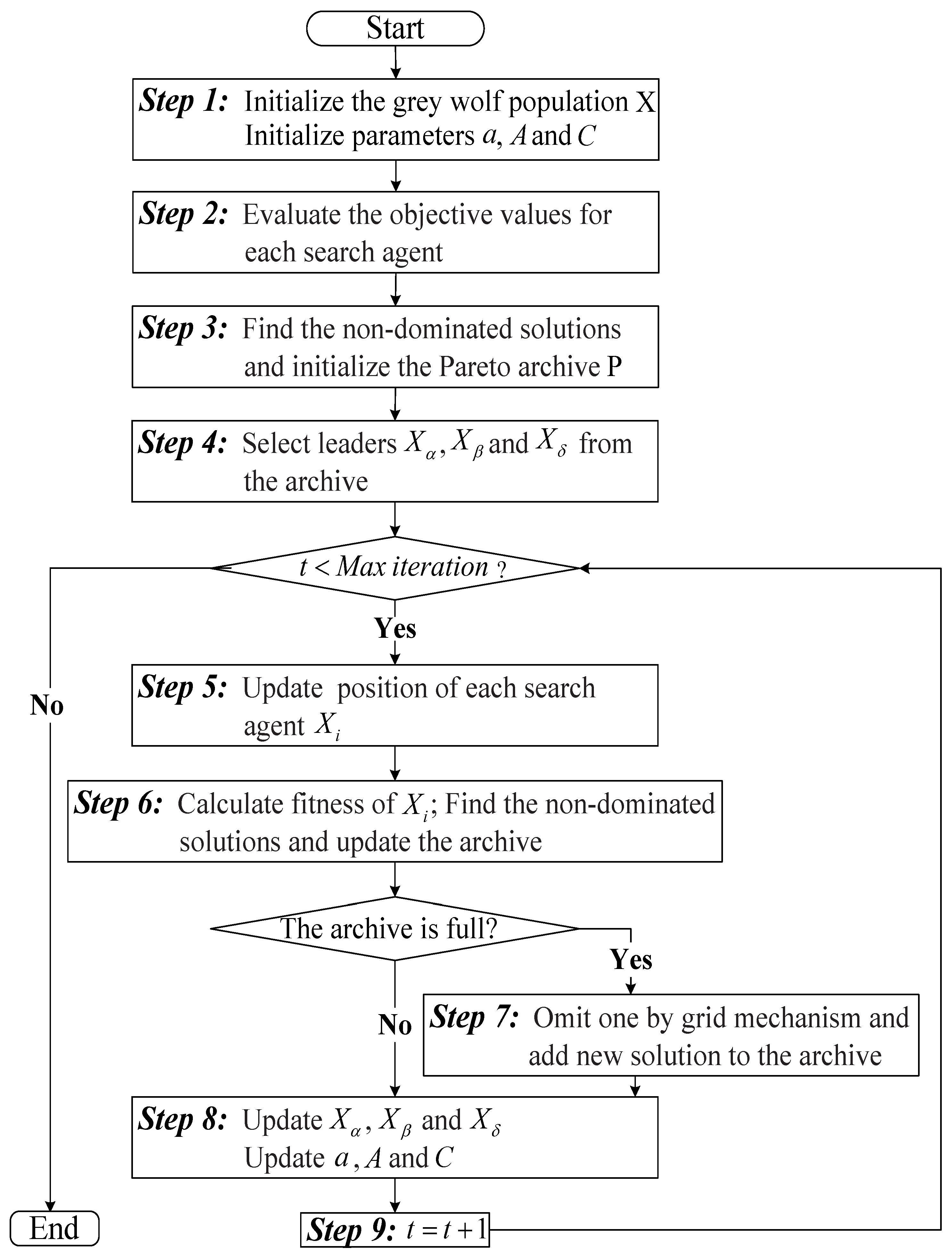
4.1. Multi-Objective Grey Wolf Optimizer (MOGWO)

As the main factor influencing vessel service schedule, the sailing speed is often optimized to give a reduction in fuel consumption and carbon emissions at the operational level. The actual sailing speeds will be dependent on three decision variables $\left(n_v,s_v,{\tau }_i\right)$ to be determined based on the proposed optimization model. Since fuel consumption approaches the third power of the sailing speed, this decision problem can be classified as a non-linear continuous procedure. A few computing methods have been proposed to solve this nonlinear speed optimization problem, but most of the previous research has only built single-objective mathematical formulations to minimize the total costs [13,46,47], while Song et al. (2015) [39] deployed a MOGA to resolve the multi-objective schedule planning problem.

In the optimization procedure, we assess three objectives (the cost, the emissions, and the unreliability) as the goal and try to obtain a very accurate approximation of Pareto optimal solutions, which refer to a set containing all of the non-dominated solutions [48]. A solution prevails over another solution on the condition that it has no worse values in all objectives and is strictly better in terms of at least one of the objectives. The non-dominated solutions denote that it is not possible to identify which one is better, and the Pareto optimal front is composed of all non-dominated solutions. Contrary to the grey wolf optimizer (GWO), it has no single solution to track when addressing the trade-offs between objectives. As a recently proposed multi-objective metaheuristic, MOGWO is extended based on GWO, which originated based on the inspiration from the hunting behaviors of grey wolves. Different from the single-objective GWO, MOGWO has integrated two new components: (1) Utilize an archive to save non-dominated Pareto optimal solutions throughout the algorithmic run; (2) Select the leader wolves from the archive.

The computational steps for MOGWO adopted in this paper are interpreted as follows and shown in Figure 4. Note that the nomenclature adopted in this subsection is independent from the one used in the model formulation and was strictly introduced to better interpret the MOGWO algorithm.

Step 1: Set the archive size $n_a=100$, the number of grey wolves $n_g=100$, and the maximum number of iterations $MaxIt=100$. Note that the values of the aforementioned parameters were set on the basis of the preliminary parameter tuning analysis. Initialize random values for $a,$ $A,$ and $C$ calculated as $A=2\cdot a\cdot r_1-a$, $C=2\cdot r_2$, where $r_1$, $r_2$ are random vectors in the $\left[\mathrm{0,1}\right]$ range and $a$ linearly falls from 2 to 0 in the process of iterations. We fix $n_v$ and $s_v$, and produce the initial grey wolf population $\left\{{\tau }_i\right\}$ from the feasible solutions.

Step 2: Assess the objective values (Cost, Emissions, and Unreliability) for each search agent.

Step 3: Obtain the non-dominated solutions and store them to an initial archive.

Step 4: Choose the three best non-dominated solutions, denoted as $\alpha$, $\beta$, and $\delta$ wolves, from the archive based on the roulette-wheel method.

Step 5: Renew the positions for the current search agent, which are computed as $D_p=C\cdot X_p\left(t\right)-X\left(t\right)$, $X\left(t+1\right)=\frac{1}{3}{\sum }_{p=\alpha ,\beta ,\gamma }\left(X_p\left(t\right)-A·D_p\right)$, where $X$ represents positions of wolves, $X_p$ denotes positions of prey; $t$ is the current iteration; $C$ and $A$ are coefficient vectors. The above equations define the encircling behavior of grey wolves. In order to hunt for prey, the $\alpha$, $\beta ,$ and $\delta$ will guide $\omega$ wolves (i.e., the other wolves in the initial population) toward promising regions located close to the prey position.

Step 6: Compute the fitness values for all search agents, obtain the non-dominated solutions from them, then compare them to the current archive, and update the archive accordingly.

Step 7: Check the number of members in the archive. If the archive is full, firstly run the grid mechanism to omit one of the current archive members; secondly, insert the new solution to the least crowded segment for increasing the diversity of the final Pareto optimal front.

Step 8: Renew the leader wolves $X_{\alpha }$, $X_{\beta }$, and $X_{\delta }$; Update $a$, $A$ and $C$.

Step 9: The iteration counter is updated as follows: $t=t+1$. This process will turn back to Step 5 and be repeated until a termination criterion is satisfied (i.e., the number of iterations reaches the maximum).

4.2. Multi-Objective Genetic Algorithm (MOGA)

To verify the effectiveness of MOGWO, we deploy the widely used multi-objective metaheuristic, non-dominated sorting GA (NSGA-II) [49], which will also be applied to the proposed multi-objective mathematical model for the vessel schedule planning problem along with MOGWO [39]. The NSGA-II is a fast and elitist MOGA, which applies a fast non-dominated sorting technique and a crowding-distance assignment to strengthen the algorithmic capabilities, so that it can maintain a diversity of Pareto optimal front sets. The elitist keeping technique used in NSGA-II guarantees that the new parent generation is performed using the best set of solutions, whereas the final non-dominant Pareto front may be remote from the true Pareto optimum during the local search.

After all, MOGWO can be theoretically more effective in contrast to other multi-objective metaheuristics in terms of the subsequent steps: (1) The best-nondominated solutions obtained thus far can be saved effectively to the external archive; (2) Only three key parameters ($a$, $A$, and $C$) need to be modified, and due to the randomness of the parameters $A$ and $C$, the alternative solutions could obtain hyper-spheres by setting different random radii; and (3) The adaptive values of the parameters $a$ and $A$ guarantee the convergence rate of MOGWO, transiting smoothly between the exploration and exploitation phases.

5. Numerical Experiments and Analysis

5.1. χ² Fit Test

The data regarding the total number of ship arrivals were adopted from the six container terminals of the Port of Shanghai for one month (29 days in February 2016). To verify whether the data gathered conform to the queuing methodology, we conducted a chi-squared test to analyze the distribution pattern of ship arrivals, taking the Zhendong Branch Company as an example (which is one of the six container terminals considered). The chi-square statistic can be calculated using Equation (28), and the results of the performed statistical analysis are displayed in

Table 1. The ${\chi }^2$ test results for ship arrival rates to the Zhendong terminal.

No. of Ship Arrivals	$\mathbf{The}\mathbf{Practical}\mathbf{Frequency}{\mathit{A}}_{\mathit{i}}$	$\mathbf{The}\mathbf{Possibility}{\mathit{p}}_{\mathit{i}}$	Chi-Square ${\mathit{\chi }}^2$
0	1	0.0136	0.9299
1	0	0.0583	1.6907
2	5	0.1254	0.5112
3	6	0.1798	0.1184
4	6	0.1933	0.0277
5	4	0.1662	0.1394
6	2	0.1191	0.6120
7	3	0.0732	0.3625
8	1	0.0393	0.0171
9	0	0.0188	0.5452
10	0	0.0001	0.0029
11	1	0.00004	—
	$Total\eta =29$	$Total=1.00$	$Total=4.9570$

. The primary (or “null”) hypothesis was assumed that the frequency distribution of the daily ship arrivals at the port follows Poisson’s distribution.

$${\chi }^2=\sum _{j=1}^g\frac{{\left(A_j-E_j\right)}^2}{E_j}=\sum _{j=1}^g\frac{{\left(A_j-\eta p_j\right)}^2}{\eta p_j}\left(j=\mathrm{1,2},3,\cdots ,g\right)$$

(28)

where $A_i$ denotes the actual frequency, $E_i$ implies the expected frequency, $\eta$ is the total frequency, and $p_i$ is the possibility of grouping $i$ under the primary hypothesis.

The degree of freedom equals the number of groups minus the number of predicted parameters and 1, presented as $DF=12-1-1=10$ (considering that were 12 ship arrivals). The confidence coefficient $\alpha$ is set to 0.05, then ${\chi }_{\alpha }^2\left(10\right)=18.31$. If ${\chi }^2<{\chi }_{\alpha }^2$, then we cannot reject the primary (or “null”) hypothesis, which confirms that the ship arrival rate follows Poisson’s distribution. Otherwise, the null hypothesis should be denied. Since the estimated ${\chi }^2$ value was found to be lower than the critical value ${\chi }_{\alpha }^2\left(10\right)$ (${\chi }^2=4.9570$), then the null hypothesis cannot be rejected; hence, the ship arrivals at the Zhendong terminal follow Poisson’s distribution.

Similar to the Zhendong terminal, the ${\chi }^2$ fit test was conducted for other five terminals located at the Port of Shanghai, including the Pudong, Hudong, Mingdong, Shengdong, and Guandong terminals. The results of additional tests are provided in

Table 2. The ${\chi }^2$ test results for ship arrival rates to six container terminals.

Company	No. of Ship Arrivals	No. of Berths	$\mathbf{When}\mathit{\alpha }=0.05$
Zhendong	124	5	${\chi }^2<{\chi }_{\alpha }^2\left(10\right)$
Pudong	112	3	${\chi }^2<{\chi }_{\alpha }^2\left(8\right)$
Hudong	182	4	${\chi }^2<{\chi }_{\alpha }^2\left(9\right)$
Mingdong	215	4	${\chi }^2<{\chi }_{\alpha }^2\left(11\right)$
Shengdong	146	9	${\chi }^2<{\chi }_{\alpha }^2\left(8\right)$
Guandong	134	7	${\chi }^2<{\chi }_{\alpha }^2\left(8\right)$

. We set $\alpha =0.05$, all ${\chi }^2<{\chi }_{\alpha }^2$, so the null hypothesis could not be rejected. Therefore, the ship arrivals at all the considered terminals of the Port of Shanghai follow Poisson’s distribution, conforming the effectiveness of the queuing methodology utilized for ships arriving at the port.

5.2. Scenario Settings

This study considered a trans-Pacific container shipping journey provided by Maersk Line [12], which was directly used to weigh the achievement of the suggested multi-objective optimization model and the algorithm. The shipping route consists of nine ports of call (and eight ports), including the subsequent ports: Kwangyang, Busan, Qingdao, Nagoya, Yokohama, Long Beach, Oakland, Dutch Harbor, Yokohama, and back to Kwangyang. The numerical data adopted throughout this study to conduct the computational experiments are provided in

Table 3. Numerical data.

Parameter	Value	Source (s)
$\mathrm{Expected}\mathrm{number}\mathrm{of}\mathrm{ship}\mathrm{arrivals}\lambda$	$U\left[\mathrm{11,13}\right]$$/U\left[\mathrm{4,6}\right]$	Gharehgozli et al. (2017) [10]
$\mathrm{Number}\mathrm{of}\mathrm{berths}c$	$U\left[\mathrm{4,6}\right]$	Gharehgozli et al. (2017) [10]
$\mathrm{Ship}\mathrm{capacity}{\phi }_v$ (TEUs)	$N\left[10000,{2000}^2\right]$	Gharehgozli et al. (2017) [10]
$\mathrm{Loading}\mathrm{and}\mathrm{unloading}\mathrm{ratios}\psi$	$U\left(\mathrm{0.1,0.3}\right)$	Gharehgozli et al. (2017) [10]
$\mathrm{Handling}\mathrm{efficiency}{r}_i$ (TEU/h)	$\left[50;75;100;125\right]$/[50;60;70;75]	Dulebenets (2018) [40]
$\mathrm{Average}\mathrm{wasted}\mathrm{time}\omega$ (mins)	50	JOC (2017) [50]
$\mathrm{Minimum}\left(\mathrm{maximum}\right)\mathrm{sailing}\mathrm{speed}{s}_{min}\left(s_{max}\right)$ (knots)	14.1 (26)	Song et al. (2015) [39]
$\mathrm{Fuel}\mathrm{price}{C}_{ho}\left(C_{do}\right)$ (USD/ton)	450 (700)	BunkerIndex (2018) [51]
Daily chartering cost for a 10,000-TEU containership (USD/day)	35,000	Clarkson (2018) [52]
$\mathrm{Vessel}\text{’}\mathrm{s}\mathrm{arrival}\mathrm{time}\mathrm{window}{W}_i$ (h)	busy ports: 4/idle ports: 6	Song et al. (2015) [39]; Lee et al. (2017) [53]
$\mathrm{Main}\mathrm{engine}\mathrm{fuel}\mathrm{economy}{F}_v^{ho}\left(F_v^{do}\right)$ (tons/h)	2.50 (0.06)	Tai and Lin (2013) [32]
$\mathrm{Carbon}\mathrm{emission}\mathrm{factor}\gamma$ (tons/ton)	3.17	Tai and Lin (2013) [32]; Buhaug et al. (2009) [54]; Liao et al. (2009) [55]; Chang and Wang (2010) [56]

.

In this experiment, we deployed five 10,000-TEU containerships to provide a weekly service, where it was assumed that ship-type $v=1$, $n_1=5$, and ${\mu }_1=\mathrm{10,000}$. Given ten voyages $K=10$, the distances between ports were used in the existing schedule, and the planned operating times for a 10,000-TEU ship at each port were computed as $l_i=2{\mu }_1\psi /r_i \left(\mathrm{h}\right)$. Similarly, the mean service time of ship-type $v$ was estimated as $u_v=2{\mu }_v{\psi }_v/24r \left(\mathrm{day}\right)$. In addition, the time wastage in the arrival and departure process time was set to 50 min at least when there were no physical restrictions [50]. The vessels were assumed to consume both heavy and light fuel oil at high sea and during the waiting period at anchorage, while only light fuel oil was assumed to be used during handling operations [32]. The main engine fuel economy by different oil types $F_v^{ho}\left(F_v^{do}\right)$ (tons/h) was set based on the data available for the ships above 7500–10,000 TEUs. The carbon emission factor was assumed to be constant for $ho$ and $do$.

Based on previous literature (Gharehgozli et al., 2017 [10]; Saeed and Larsen, 2016 [29]; Dulebenets, 2018 [40]), the ports of call could be defined as ‘larger ports’ if they were listed in the ‘Top 20 world container ports’ and ‘smaller ports’ otherwise. Then, we adopted some basic settings and assumptions to calculate the queuing time, on the basis of the data shown in Table 3. The following parameters could be generated based on different uniform distributions: the expected number of ship arrivals $\lambda ~U\left[\mathrm{11,13}\right]$/$U\left[\mathrm{4,6}\right]$, the number of berths $c~U\left[\mathrm{4,6}\right]$, the loading and unloading ratios $\psi ~U\left(\mathrm{0.1,0.3}\right)$, where the loading and unloading volumes are equal. The sizes of ships were assumed to follow the normal distribution ${\mu }_v~N\left[10000,{2000}^2\right]\mathrm{TEUs}$, where mainly five types of ships were expected to arrive at ports. The container handling rates were set to $r_i\left[50;75;100;125\right]\mathrm{TEUs}/\mathrm{h}$ or $r_i\left[50;60;70;75\right]\mathrm{TEUs}/\mathrm{h}$ according to different congestion situations. Let the arrival time window be $W_i=4 \mathrm{h}$ or $W_i=6 \mathrm{h}$ for any busy (idle) ports.

Two multi-objective metaheuristics that were used in this study, MOGWO and NSGA-II, were both carried out applying Matlab running on a PC with an Intel Core i5 processor (2.30 GHz) and 8 GB RAM. In the MOGWO, the archive size was set to 100, the number of grey wolves was set to 100, and the maximum number of iterations was restricted to 1000. In the NSGA-II, the population size was fixed to 100, the mutation ratio was fixed to 0.02, and the maximum number of generations was restricted to 1000. Note that the values of the aforementioned parameters were set on the basis of the preliminary parameter-tuning analysis for MOGWO and NSGA-II. The averaged performance metric values were obtained through 15 time runs for each algorithm.

The following sections discuss the achieved performance of the model and the algorithm in three groups of experiments. In the first group, two queuing theories: $M/M/1$ and $M/M/c$, were applied to calculate the queuing times at ports, and the results under two queuing systems were compared. Then, we compared the two proposed solution methods and illustrated the impacts of decision variables on the considered objective functions under the basic assumptions. Furthermore, the Pareto optimal solutions from the better method were analyzed for differing values of fuel price and berth occupancy rate in order to examine the impacts of key factors on the three objectives.

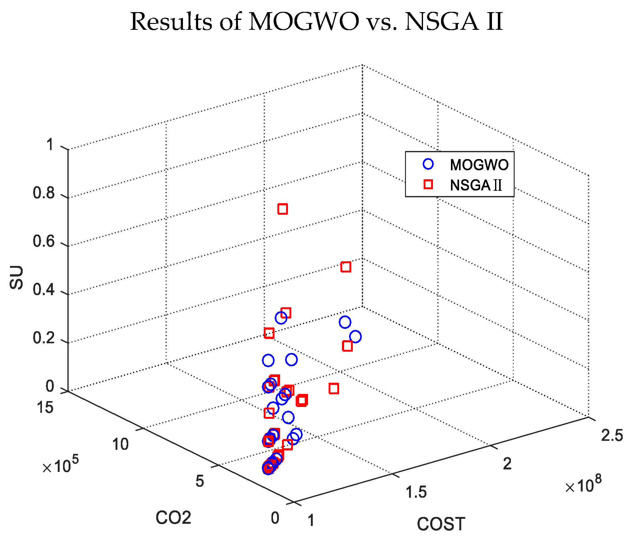
5.3. Computational Results

In this section, we examined the Pareto optimal sets acquired by MOGWO and NSGA-II in contrast to check the effectiveness of the algorithms. Based on the basic parameter settings above, we let $n_v=\{4,5,6,7,8,9\}$ and $s_v=\{15,18,20,23,26\}$. For various combined groups of $n_v$ and $s_v$, the experimental results applying the two queuing theories with MOGWO were compared in

Table 4. Computational results with $M/M/1$ queuing theory–MOGWO.

	Min COST			CPU Time (s)	Min CO2			CPU Time (s)	Min SU			CPU Time (s)
	COST ($)	CO2 (tons)	SU (%)		COST ($)	CO2 (tons)	SU (%)		COST ($)	CO2 (tons)	SU (%)
$n_v$	$s_v=26$
5	198,845,792	953,743	22.5	276.8	198,845,792	953,743	22.6	295.8	210,299,255	1,032,856	11	312.1
6	139,875,293	538,721	33.7	297.5	139,875,293	538,721	33.7	262.9	144,793,425	570,023	0	293.2
7	119,176,237	396,742	0	258.2	119,176,237	396,742	0	273.1	119,176,237	397,529	0	289.5
8	116,043,260	369,379	11	303.9	116,043,260	369,379	11	301.9	118,437,429	384,592	0	291.2
9	113,871,396	354,738	0	297.5	113,871,396	354,738	0	278.3	113,875,303	353,190	0	286.1
$n_v$	$s_v=23$
6	132,581,521	485,432	22.5	305.7	132,581,521	485,432	22.7	274.5	141,317,289	546,742	0	293.4
7	117,536,973	379,209	0	295.6	117,536,973	379,209	0	285.7	117,526,781	379,568	0	297.1
8	115,289,727	363,576	11	296.2	115,289,727	363,576	11	289.8	115,532,980	365,341	0	274.3
9	114,042,975	353,709	0	283.9	114,042,975	353,709	0	292.2	114,041,289	35,709	0	286.9
$n_v$	$s_v=20$
6	128,794,567	458,209	22	312.6	128,794,567	458,209	22	281.9	135,881,809	508,029	11	281.3
7	119,551,283	393,129	22	309.1	119,551,283	393,129	22	273.8	122,652,891	415,901	0	271.8
8	114,152,709	355,190	11	268.3	114,152,709	355,190	11	276.9	118,052,132	382,318	0	287.9
9	113,832,781	352,771	0	256.3	113,832,781	352,771	0	291.2	113,837,819	353,110	0	245.1
$n_v$	$s_v=18$
6	128,931,249	459,231	56.9	281.3	128,931,249	459,231	57	271.4	128,929,170	459,243	57.1	291.8
7	116,829,817	373,742	33.9	235.7	116,829,817	373,742	33.4	275.3	119,189,451	389,798	11	259.8
8	114,398,028	359,450	0	280.3	114,398,028	359,450	0	273.8	114,397,688	35,610	0	278.5
9	113,837,891	353,142	0	292.5	113,837,891	353,142	0	273.5	113,834,123	352,579	0	269.8
$n_v$	$s_v=15$
7	114,319,725	356,328	45	273.5	114,319,725	356,328	44.9	286	114,319,725	356,328	33	239.7
8	113,838,694	353,172	0	287.2	113,838,694	353,172	0	272.1	113,838,694	353,172	0	297.3
9	113,838,694	353,172	0	280.1	113,838,694	353,172	0	276.5	113,838,694	353,172	0	282.1

and

Table 5. Computational results with $M/M/c$ queuing theory–MOGWO.

	Min COST			CPU Time (s)	Min CO2			CPU Time (s)	Min SU			CPU Time (s)
	COST ($)	CO2 (tons)	SU (%)		COST ($)	CO2 (tons)	SU (%)		COST ($)	CO2 (tons)	SU (%)
$n_v$	$s_v=26$
5	198,836,964	950,957	22	273.1	198,836,964	950,957	22	284.2	210,298,399	1,031,697	11	305.9
6	139,861,951	535,511	33	263.3	139,861,951	535,511	33	263.1	144,751,373	569,954	0	287.2
7	119,165,893	389,719	0	285.9	119,165,893	389,719	0	289.3	119,165,893	389,719	0	275.8
8	116,030,160	367,629	11	294.3	116,030,160	367,629	11	302.2	118,416,911	384,442	0	268.7
9	113,869,903	352,096	0	301.8	113,869,903	352,096	0	298.1	113,869,903	352,096	0	267.9
$n_v$	$s_v=23$
6	132,570,091	484,144	22	295.3	132,570,091	484,144	22	267.3	141,305,733	545,682	0	283.2
7	117,514,984	378,089	0	284.1	117,514,984	378,089	0	278.5	117,514,984	378,089	0	287.1
8	115,287,658	362,399	11	285.4	115,287,658	362,399	11	279.8	115,521,633	364,047	0	269.5
9	114,038,902	353,602	0	273.8	114,038,902	353,602	0	281.5	114,038,902	353,602	0	278.3
$n_v$	$s_v=20$
6	128,793,787	457,542	22	305.2	128,793,787	457,542	22	269.4	135,875,406	507,113	11	296.1
7	119,547,195	392,405	22	304.1	119,547,195	392,405	22	268.3	122,641,977	414,206	0	297.3
8	114,146,407	354,359	11	296.2	114,146,407	354,359	11	285.1	118,041,516	381,798	0	295.3
9	113,825,165	352,096	0	297.1	113,825,165	352,096	0	287.5	113,825,165	352,096	0	296.3
$n_v$	$s_v=18$
6	128,927,798	458,171	56	279.2	128,927,798	458,171	56	269.3	128,927,798	458,171	56	289.5
7	116,823,463	372,902	33	268.3	116,823,463	372,902	33	281.5	119,183,279	389,526	11	293.4
8	114,396,338	355,805	0	285.1	114,396,338	355,805	0	285.3	114,396,338	355,805	0	293.0
9	113,825,165	352,096	0	269.7	113,825,165	352,096	0	283.4	113,825,165	352,096	0	289.8
$n_v$	$s_v=15$
7	114,307,116	355,491	44	269.0	114,307,116	355,491	0.4444	299.3	114,377,076	355,984	33	296.8
8	113,825,165	352,096	0	283.2	113,825,165	352,096	0.0000	289.0	113,825,165	352,096	0	268.3
9	113,825,165	352,096	0	276.5	113,825,165	352,096	0.0000	297.3	113,825,165	352,096	0	291.0

. Compared with assigning berths based on the $M/M/1$ policy in Table 4, it is more efficient to allocate public berths to ships stochastically using $M/M/c$ in Table 5, which could obtain lower costs and carbon emissions, and also a higher service reliability. Therefore, we applied $M/M/c/N/\infty$ to calculate the queuing times at ports firstly, and then executed both metaheuristics for different combinations of $n_v$ and $s_v$. The experimental results with the obtained MOGWO and NSGA-II solutions $n_v$, $s_v$ are presented in Table 5 and

Table 6. Computational results with $M/M/c$ queuing theory–NSGA-II.

	Min COST			CPU Time (s)	Min CO2			CPU Time (s)	Min SU			CPU Time (s)
	COST ($)	CO2 (tons)	SU (%)		COST ($)	CO2 (tons)	SU (%)		COST ($)	CO2 (tons)	SU (%)
$n_v$	$s_v=26$
5	200,068,969	959,636	44	677.5	200,068,969	959,636	44	643.4	201,399,247	969,007	11	651.4
6	152,320,338	622,958	11	643.8	152,320,338	622,958	11	684.1	186,994,507	867,218	0	682.3
7	124,364,311	426,023	0	653.7	124,364,311	426,023	0	692.7	124,364,311	426,023	0	691.4
8	119,083,322	388,822	0	649.1	119,083,322	388,822	0	644.0	119,083,322	388,822	0	671.3
9	113,960,518	353,050	0	653.8	113,960,518	353,050	0	692.1	113,960,518	353,050	0	682.9
$n_v$	$s_v=23$
6	134,778,503	499,386	22	674.2	134,778,503	499,386	22	684.1	150,745,194	611,862	11	667.3
7	120,369,192	397,880	11	669.2	120,369,192	397,880	11	691.9	135,647,581	505,508	0	682.2
8	116,181,824	368,382	11	673.8	116,181,824	368,382	11	685.6	116,516,878	370,743	0	691.0
9	114,845,060	358,966	0	681.7	114,845,060	358,966	0	645.0	114,845,060	358,966	0	689.1
$n_v$	$s_v=20$
6	133,570,541	490,876	56	682.5	133,570,541	490,876	56	652.0	136,668,643	512,701	22	693.0
7	121,314,125	404,537	33	689.4	121,314,125	404,537	33	653.0	125,899,408	436,837	0	667.2
8	115,244,387	361,779	22	672.5	115,244,387	361,779	22	666.2	118,182,647	382,477	0	663.2
9	114,154,602	354,102	0	675.8	114,154,602	354,102	0	692.1	114,154,602	354,102	0	682.3
$n_v$	$s_v=18$
6	129,914,312	465,120	100	690.2	129,914,312	465,120	100	684.3	129,914,312	465,120	100	681.4
7	119,980,723	395,144	33	683.5	119,980,723	395,144	33	674.5	120,835,603	401,166	11	665.3
8	115,708,515	365,048	0	675.9	115,708,515	365,048	0	685.6	115,708,515	365,048	0	671.8
9	114,002,427	353,030	11	677.4	114,002,427	353,030	11	690.9	114,338,240	355,395	0	693.0
$n_v$	$s_v=15$
7	114,530,757	356,752	56	682.0	114,530,757	356,752	56	680.8	114,541,963	356,830	33	682.3
8	113,926,911	352,498	0	680.1	113,926,911	352,498	0	657.1	113,926,911	352,498	0	660.5
9	113,870,770	352,102	0	652.1	113,870,770	352,102	0	646.2	113,870,770	352,102	0	648.7

. Moreover, Figure 5 shows the identical combination of solutions in a three-dimensional space.

Based on the obtained results, MOGWO can obtain better Pareto solutions compared to NSGA-II under each scenario of $n_v$ and $s_v$. The four columns present the objective function values under each best single objective and runtime. Therefore, we can conclude that our proposed MOGWO deployed for the green vessel scheduling model can obtain better objective values than the NSGA-II used by Song et al. (2015) [39]. A couple of observations from the results are noteworthy. For both metaheuristic approaches, the best $COST$ and ${CO}_2$ values can be obtained simultaneously, and they have the same variation trend of decreasing with the increase in $n_v$ under each fixed $s_v$. The best $COST$ and ${CO}_2$ values have a declining trend with not only the increased vessel number but also with the decrease in planned speed. The best $SU$ values do not seem to have a clear relationship with $n_v$ and $s_v$. However, the best $SU$ values are generally observed for the scenarios with a larger number of deployed vessels, which implies sufficient transit time. Note that there can be an abrupt change to the $SU$ objective when adding $n_v$ from 6 to 7 with fixed $s_v=18$ (e.g., MOGWO has a sharp decline from 56% to 11%, while NSGA-II decreases from 100% to 11%). For some cases of MOGWO and NSGA-II, $n_v=5$, $s_v=23$ could not obtain any solution due to the insufficient number of deployed vessels.

By comparing Table 5 and Table 6, it can be concluded that the solutions attained by utilizing MOGWO are up to 4%, 6%, and 44% better than the ones generated by NSGA-II for the $COST$, ${CO}_2$, and $SU$ objectives, respectively. Specifically, MOGWO achieves the min $COST$ value ($USD\mathrm{113,825,165}$) and ${CO}_2$ value ($\mathrm{352,096}\mathrm{tons}$) when $n_v=9$ and $s_v=15$, while NSGA-II obtains the min $COST$ value ($USD\mathrm{113,870,770}$) and ${CO}_2$ value ($\mathrm{352,102}\mathrm{tons}$) for the same $n_v=9$ and $s_v=15$; hence, the difference between them can be viewed as quite small. However, a bigger difference can be observed when considering the relatively worse $COST$ values ($USD\mathrm{201,399,247}$ vs $USD\mathrm{210,298,399}$) and ${CO}_2$ values ($\mathrm{969,007}\mathrm{tons}$ vs $\mathrm{1,031,697}\mathrm{tons}$) when $n_v=6$ and $s_v=18$. It can be seen that both the $COST$ and ${CO}_2$ objectives are more dominated by the MOGWO solution located closer to the left-bottom corner, which is more obviously visualized in Figure 5. Moreover, the CPU runtime of MOGWO was on average twice as fast than that of NSGA-II for 1000 iterations.

Table 7. Top 20 Pareto solutions of MOGWO under the basic setting.

COST ($)	CO2 (tons)	SU (%)	${\mathit{n}}_{\mathit{v}}$	${\mathit{s}}_{\mathit{v}}$ (knots)	$\left\{{\mathit{\tau }}_{\mathit{i}}, \mathit{i} = \mathrm{1,2},\dots ,\mathit{N}\right\}$ (h)	$\left\{{\mathit{s}}_{\mathit{i}}, \mathit{i} = \mathrm{1,2},\dots ,\mathit{N}\right\}$ (knots)
113,825,165	352,096	0	9	20	{132,70,138,81,378,62,231,222,222}	{14.1,14.1,14.1,14.1,14.1,14.1,14.1,14.1,14.1}
113,869,903	352,096	0	9	20	{94,93,176,53,391,104,186,248,223}	{14.1,14.1,14.1,14.1,14.1,14.1,14.1,14.1,14.1}
113,936,131	352,878	33	8	15	{124,228,105,100,354,42,197,330,57}	{14.1,14.1,14.1,14.1,14.1,14.1,14.1,14.1,14.1}
113,974,212	353,146	22	8	15	{118,89,111,89,284,211,182,229,84}	{14.1,14.1,14.1,14.1,14.1,14.1,14.1,14.1,14.1}
114,038,902	353,602	0	9	18	{33,74,100,71,356,97,361,280,140}	{14.1,14.1,15.4,14.1,14.5,14.1,14.1,14.1,14.1}
114,146,407	354,359	11	8	20	{354,249,104,37,366,118,232,213,132}	{19.3,14.1,14.6,14.1,14.1,14.1,14.1,14.1,14.1}
114,307,116	355,491	44	7	15	{181,68,108,41,210,175,199,214,59}	{14.1,15,15,14.1,14.5,14.1,15,15,14.1}
114,377,076	355,984	33	7	15	{110,204,106,37,164,194,256,204,31}	{14.1,14.6,14.1,14.1,15,15,14.1,14.8,15}
114,396,338	355,805	0	8	18	{236,90,112,100,340,82,188,273,80}	{14.1,14.1,14.1,14.1,15.2,14.1,14.1,14.1,14.5}
114,476,122	356,682	44	7	15	{291,74,73,55,153,298,146,255,78}	{14.1,14.1,14.3,14.1,15,15,14.6,15,15}
114,583,222	357,436	33	7	15	{14,203,103,50,172,185,235,147,151}	{14.1,14.1,14.1,14.1,14.1,15, 15,15,15}
115,287,658	362,399	11	8	23	{292,180,95,96,352,82,164,242,191}	{22,14.1,16.6,14.1,14.7,14.1,14.8,14.1,14.1}
115,521,633	364,047	0	8	23	{208,89,149,69,325,113,160,292,97}	{14.1,14.1,14.1,14.1,16,14.1,15.2, 14.1,14.1}
115,592,605	364,547	22	8	18	{197,122,103,51,333,228,192,180,77}	{14.1,14.1,16.6,14.1,16,14.1,15.2,14.1,14.1}
116,120,133	368,263	0	8	18	{218,183,95,151,324,64,160,211,92}	{14.1,14.1,16.6,14.1,16,14.1,15.1,14.1,14.1}
116,823,463	372,902	33	7	18	{193,175,97,88,303,46,163,202,151}	{17.6,17.6,17.6,14.1,15.5,14.1,14.1,14.5,14.1}
118,041,516	381,798	0	8	20	{17,146,182,34,304,100,163,197,107}	{14.8,14.1,14.1,15.2,17.1,14.1,15,15.2,14.1}
114,171,243	354,534	11	9	20	{62,61,112,157,342,51,302,295,129}	{19.3,14.1,14.1,14.1,14.4,14.1,14.1,14.1,14.1}
114,431,927	356,370	0	9	20	{360,170,171,38,426,108,186,259,193}	{14.1,14.1,14.4,14.1,15.3,14.1,14.1,14.1,14.1}
116,030,160	367,629	11	8	26	{13,290,110,34,336,75,238,247,187}	{26,14.1,14.1,15.7,15.4,14.1,14.1,14.1,14.1}

and

Table 8. Top 20 Pareto solutions of NSGA-II under the basic setting.

COST ($)	CO2 (tons)	SU (%)	${\mathit{n}}_{\mathit{v}}$	${\mathit{s}}_{\mathit{v}}$ (knots)	$\left\{{\mathit{\tau }}_{\mathit{i}}, \mathit{i} = \mathrm{1,2},\dots ,\mathit{N}\right\}$ (h)	$\left\{{\mathit{s}}_{\mathit{i}}, \mathit{i} = \mathrm{1,2},\dots ,\mathit{N}\right\}$ (knots)
113,870,770	352,102	0	9	15	{207,247,74,125,204,100,152,200,204}	{14.1,14.1,14.1,14.1,14.1,14.1,14.1,14.1,14.1}
113,902,053	352,323	22	9	15	{95,80,200,23,321,172,42,400,203}	{14.1,14.1,14.1,14.1,14.1,14.1,14.1,14.1,14.1}
113,926,911	352,498	0	8	15	{338,157,88,87,24,233,302,106,42}	{14.1,14.1,14.1,14.1,14.5,14.1,14.1,14.1,14.1}
113,960,518	353,050	0	9	26	{127,79,152,64,352,65,235,328,186}	{14.1,14.1,14.1,14.1,14.7,14.1,14.1,14.1,14.1}
113,967,387	352,783	33	8	15	{314,20,115,211,30,37,229,246,142}	{14.9,14.9,14.1,14.1,14.1,14.1,14.1, 14.1,15}
114,002,427	353,030	11	9	18	{200,230,272,53,100,212,11,242,192}	{19.6,14.1,14.1,14.1,14.1,14.1,14.1,14.1,14.1}
114,154,602	354,102	0	9	20	{144,142,163,196,139,247,225,64,192}	{14.1,14.1,14.1,14.1,14.9,14.1,14.1,14.1,14.1}
114,173,055	354,232	11	9	20	{90,264,77,351,143,110,84,281,112}	{20,14.1,14.1,14.1,14.1,14.1,14.1, 14.1,14.1}
114,338,240	355,395	0	9	18	{98,195,223,258,184,51,43,236,223}	{14.1,14.1,14.1,14.1,14.1,18,14.1,14.1,14.1}
114,530,757	356,752	56	7	15	{167,151,88,116,146,131,65,118,194}	{14.1,14.6,15,15,15,14.1,14.1,15,15}
114,541,963	356,830	33	7	15	{193,206,36,135,227,69,163,99,48}	{14.1,14.1,15,14.2,15,15,14.7,15,14.1}
114,845,060	358,966	0	9	23	{42,247,65,185,125,297,302,100,148}	{14.1,14.1,14.1,14.1,15.6,14.1,14.1,14.1,14.1}
115,244,387	361,779	22	8	20	{244,87,193,139,105,48,151,164,213}	{19.5,14.1,14.1,14.1,14.1,20,14.1,14.1,14.1}
115,373,967	362,691	11	9	23	{188,210,267,163,120,15,242,267,40}	{23,14.1,14.1,14.1,15.5,14.1,14.1,14.1,14.1}
115,708,515	365,048	0	8	18	{258,142,76,72,228,99,22,184,263}	{14.1,14.1,14.1,14.1,16.2,14.1,14.1,14.3,14.1}
116,181,824	368,382	11	8	23	{180,157,184,186,168,35,47,213,205}	{22.1,14.1,14.1,14.1,16.1,14.1,14.1,14.1,14.1}
116,516,878	370,743	0	8	23	{46,146,265,197,100,23,266,212,88}	{14.1,14.1,14.1,15.2,16.6,14.1,14.1,14.1,14.1}
116,922,940	373,603	11	8	18	{65,121,18,107,290,240,110,207,196}	{14.1,14.1,18,14.1,16.1,14.1,14.1,14.1,14.1}
118,182,647	382,477	0	8	20	{106,82,162,55,104,148,243,230,215}	{14.8,14.8,14.8,14.1,17.3,14.1,14.1,14.1,14.1}
119,083,322	388,822	0	8	26	{182,384,158,227,64,202,46,39,42}	{14.1,14.1,14.1,14.1,17.7,14.1,14.1,14.1,14.1}

give the top 20 Pareto solutions (which have superior Pareto fronts) and the decision variables of MOGWO and NSGA-II after running each algorithm 15 times for each combination of $n_v$ and $s_v$, where $s_i$ denotes the average sailing speed over 10 voyages on each leg. A couple of interesting implications can be denoted. Firstly, the objective values in the MOGWO solution set range from $USD\mathrm{113,825,165}$ to $USD\mathrm{118,041,516}$ ($COST$), $\mathrm{352,096}\mathrm{tons}$ to $\mathrm{381,798}\mathrm{tons}$ (${CO}_2$), and 0 to 44% ($SU$), while the objective values in the NSGA-II solution set range from $USD\mathrm{113,870,770}$ to $USD\mathrm{119,083,322}$, $\mathrm{352,102}\mathrm{tons}$ to $3888\mathrm{tons}$, and $0$ to $56\%$. These results also imply that MOGWO can generate higher quality solutions. Secondly, it can also be observed that the number of deployed vessels has a narrow range (7–9 vessels), while the planned speed ranges widely from $15\mathrm{knots}$ to $26\mathrm{knots}$. However, most of the practical sailing speeds are closer to the lowest bound ($14.1\mathrm{knots}$). Especially, the best $COST$ and ${CO}_2$ objectives are all associated with $14.1\mathrm{knots}$ for the solutions produced by MOGWO ($n_v=9, s_v=20$; $n_v=9, s_v=26;n_v=8, s_v=15$) and by NSGA-II ($n_v=9, s_v=15$). Note that in the cases when $n_v=9, s_v=18$; $n_v=8, s_v=15$; and $n_v=9, s_v=15$, the dominated solutions can also be obtained using MOGWO. This may imply that the cost and emission performances are sensitive to the sailing speed, which justifies slow steaming as an operational practice to save fuel regardless of whether the vessels have been delayed. Thirdly, the optimal number of deployed vessels is 8 in 19 of 40 cases. Deploying 7–9 vessels can obtain better solutions in terms of the considered objectives than those deploying 5–6 vessels in all cases.

Two additional points should be highlighted. The lower levels of sailing speed ($s_v=15,18$) were adopted when $n_v=7$ with a positive service unreliability, whereas the deployment of 9 vessels had a wide range of speed choices with high customer satisfaction, and many of them adopted high speed levels. Moreover, fewer vessels had a shorter voyage time (sum of the transit times). For instance, the voyage time ranged from $1124\mathrm{h}$ to $1423\mathrm{h}$ in Table 7 and $1165\mathrm{h}$ to $1176\mathrm{h}$ in Table 8 when $n_v=7$, but it ranged from $1511\mathrm{h}$ to $1911\mathrm{h}$ and $151\mathrm{h}$ to $151\mathrm{h}$ when $n_v=9$. This finding could be interpreted as fewer vessels being required to provide the weekly service frequency at ports when sailing at high speeds. However, when shipping operators prefer to slow the vessels down to decline the total cost and carbon emission, the schedule reliability could be negatively affected. Nevertheless, an insufficient number of vessels (e.g., $n_v=5,6$) cannot provide schedule reliability against uncertainties even when sailing at high speeds, which will cause high fuel consumption in the meanwhile. To sum up, allocating the optimal number of vessels in the mid-term planning should be considered as the primary measure, and then adjusting the speed selection strategy to absorb various uncertainties could be adopted as an operational measure. For shipping lines, the buffer times on sailing legs should be considered to combat the negative effects of the uncertain port times, thus preventing arriving too early at a busy container terminal by adjusting the sailing speed, which leads to an improved service reliability and reduced fuel consumption and emissions in the sailing period. For port operators, variable vessel arrivals should also be considered in advance when allocating berth resources, which helps to control vessel emissions in the mooring period.

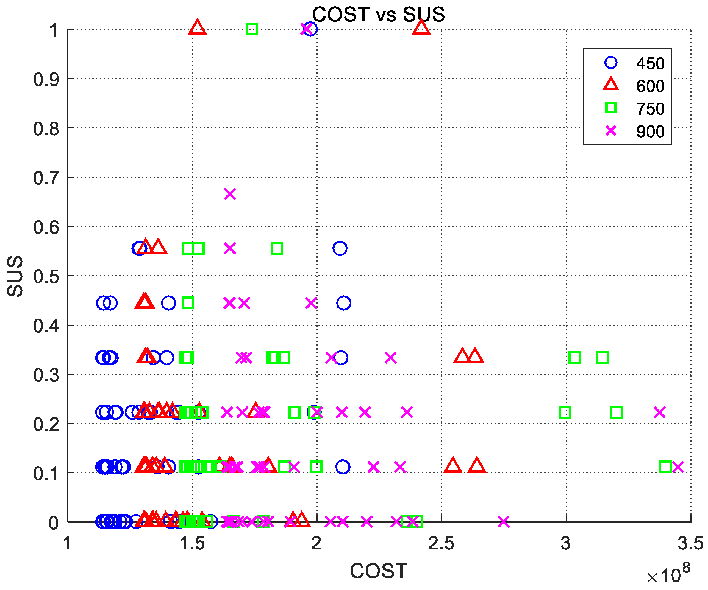
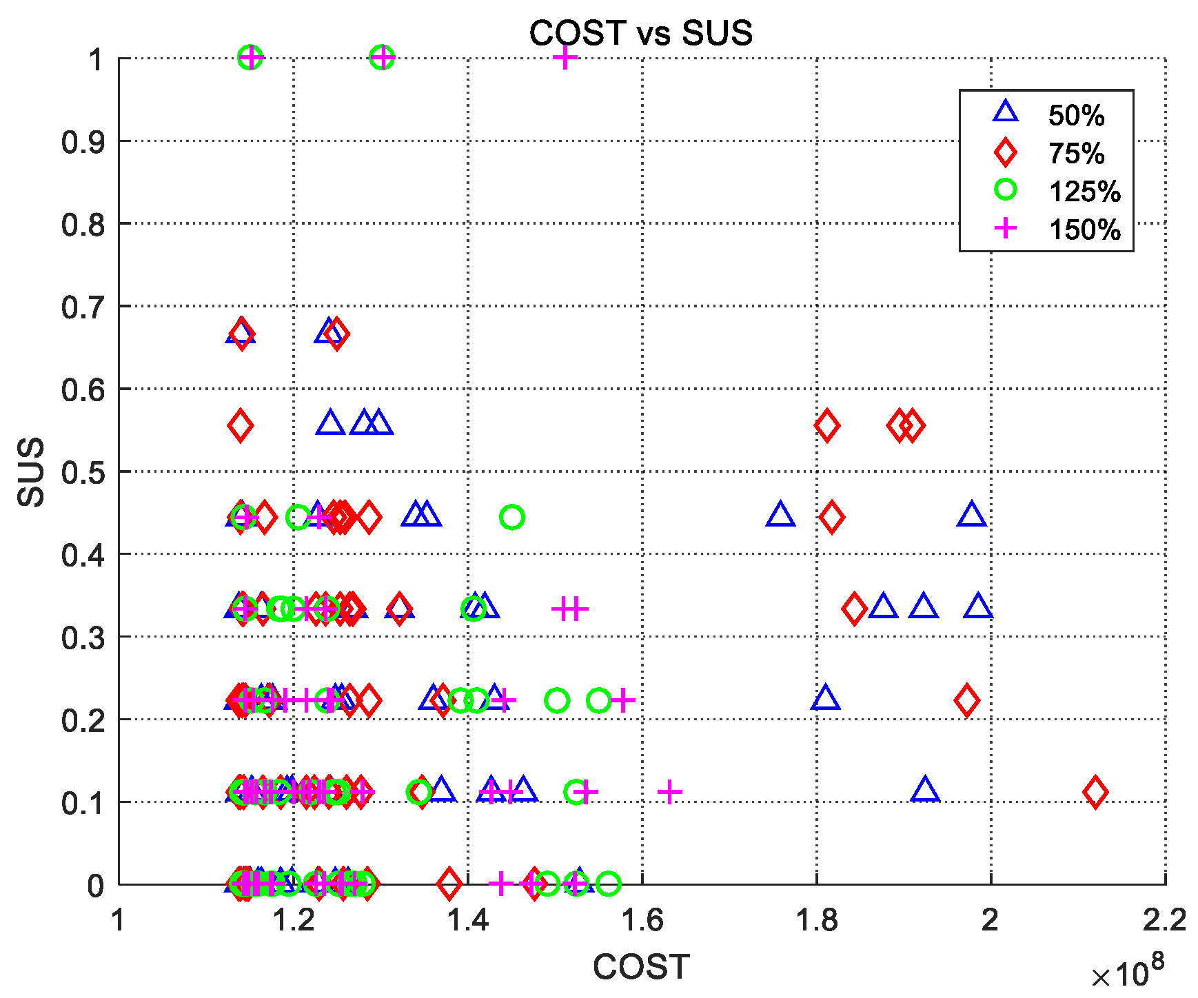
5.4. Sensitivity Analysis

In this section, we present sensitivity analyses with two groups of parameters. One of the most important parameters in vessel scheduling is the fuel unit cost, which affects the operational cost of shipping and has fluctuated recently. Therefore, a sensitivity analysis with fuel prices was performed for different values of the fuel unit cost, including $450\mathrm{USD}/\mathrm{ton}$, $600\mathrm{USD}/\mathrm{ton}$, $750\mathrm{USD}/\mathrm{ton},$ and $900\mathrm{USD}/\mathrm{ton}$. Here, $750\mathrm{USD}/\mathrm{ton}$ and $900\mathrm{USD}/\mathrm{ton}$ represent the unit cost of very-low sulphur fuel oil (VLSFO), which is used to replace HFO outside ECAs (emission control areas) since 2020 for conforming with the IMO emission regulations. Figure 6, Figure 7, Figure 8 and Figure 9 visualize the 60 best obtained results subject to different fuel prices ($450\mathrm{USD}/\mathrm{ton}$, $600\mathrm{USD}/\mathrm{ton}$, $750\mathrm{USD}/\mathrm{ton}$, and $900\mathrm{USD}/\mathrm{ton}$) generated by MOGWO, including the Pareto fronts in a three-dimensional space (Figure 6) and trade-offs between each pair of two objectives in two-dimensional space (Figure 7, Figure 8 and Figure 9).

Among all of the solutions under combinations of $n_v$ and $s_v$ for different fuel prices, each combination was evaluated for 15 run times using MOGWO. The cost ranged from $USD\mathrm{113,825,165}$ to $USD\mathrm{227,826,362}$, and the carbon emission ranged from $\mathrm{352,096}\mathrm{tons}$ to $\mathrm{1,155,171}\mathrm{tons}$ when $C_{ho}=450$; the cost ranged from $USD\mathrm{130,522,927}$ to $USD\mathrm{294,422,199}$, and the carbon emission ranged from $\mathrm{352,096}\mathrm{tons}$ to $\mathrm{1,218,031}\mathrm{tons}$ when $C_{ho}=600$; the cost ranged from $USD\mathrm{147,175,951}$ to $USD\mathrm{339,854,554}$, and the carbon emission ranged from $\mathrm{352,096}\mathrm{tons}$ to $\mathrm{1,166,484}\mathrm{tons}$ when $C_{ho}=750$; the cost ranged from $USD\mathrm{163,828,976}$ to $USD\mathrm{353,034,474}$, and the carbon emission ranged from $\mathrm{352,096}\mathrm{tons}$ to $\mathrm{1,018,520}\mathrm{tons}$ when $C_{ho}=900$; and all of the schedule unreliability ranged anywhere from $0$ to $100\%$. The subsequent observations can be obtained from the computational results: (1) the cost value increases by $44\%$ to $55\%$, while the CO₂ increases by $5.4\%$ then decreases by $16\%$ as the fuel prices increase $100\%$ (from $450\mathrm{USD}/\mathrm{ton}$ to $900\mathrm{USD}/\mathrm{ton}$); and (2) as illustrated in Figure 6 and Figure 7, with the fuel price is rising, the sharp slope of the Pareto front and the CO₂–COST curve turns into a moderate slope, which means that the changes in emissions become less substantial than the cost changes. The best emission value is constant even with different fuel prices and can be obtained together with the best cost value. However, the variation in emissions can give some insights to the shipping industry, as the increasing bunker unit cost or fuel surcharge or adopting VLSFO can have a positive impact in terms of reducing carbon emissions only to a certain extent, although with an increase in cost.

Similar $n_v$, $s_v$ to the results in Section 5.3, it can be seen that the voyage time was shorter when deploying 7 vessels. However, the optimal value of $n_v$ was found to be 9 and all values of $s_i$ were below 20 in the top 20 solutions for higher fuel prices. This can be analyzed through the causes that the vessel operators had no other choice but to use slow steaming in order to control cost, and even deploy more vessels to maintain the service reliability. The operating cost of adding one more vessel was not as significant as the bunker cost of speeding up vessels when the fuel price was higher. As shown in Figure 8 and Figure 9, the service unreliability was quite sensitive to carbon emissions compared to the cost in the top 60 Pareto solutions, as the variation in carbon emissions was smaller than the variation in cost. The solutions were found to be more disjointed and sparser with $C_{ho}=900$ than those with $C_{ho}=450$. Meanwhile, the negative relationship between unreliability and cost (emissions) fluctuates more heavily with the increase in fuel price. Such a finding can be explained by the fact that deploying more vessels under high fuel prices can not only control bunker costs and carbon emissions but also maintain customer satisfaction with the shipping service.

The berth occupancy rate for different container terminals in various periods could also change. Another group of sensitivity analyses was conducted for different occupancy rates. Here, 50%, 75%, 125%, and 150% represent different variation degrees in vessel service intensities in relation to the basic setting. Figure 10, Figure 11, Figure 12 and Figure 13 illustrate the 60 best obtained results subject to different service intensities generated by MOGWO, including the Pareto fronts and trade-offs between each pair of two objectives.

For each case under the combination of $n_v$ and $s_v$ for different service intensity scenarios, MOGWO was executed 15 times in order to obtain the Pareto fronts. It was found that the cost ranged from $USD\mathrm{113,662,002}$ to $USD\mathrm{211,855,561}$, the carbon emission ranged from $\mathrm{350,650}\mathrm{tons}$ to $\mathrm{1,042,370}\mathrm{tons}$, and the service unreliability ranged from $0$ to $67\%$ when the occupancy rate was set to $50\%$ of the base case; the cost ranged from $USD\mathrm{113,668,147}$ to $USD\mathrm{213,183,148}$, the carbon emission ranged from $\mathrm{350,693}\mathrm{tons}$ to $\mathrm{1,051,721}\mathrm{tons}$, and the service unreliability ranged from $0$ to $67\%$ when the occupancy rate was set to $75\%$ of the base case; the cost ranged from $USD\mathrm{114,068,400}$ to $USD\mathrm{263,304,166}$, the carbon emission ranged from $\mathrm{353,477}\mathrm{tons}$ to $\mathrm{1,404,760}\mathrm{tons}$, and the service unreliability ranged from $0$ to $100\%$ when the occupancy rate was set to $125\%$ of the base case; the cost ranged from $USD\mathrm{114,362,577}$ to $USD\mathrm{263,598,343}$, the carbon emission ranged from $\mathrm{355,522}\mathrm{tons}$ to $\mathrm{1,406,805}\mathrm{tons}$, and the service unreliability ranged from $0$ to $100\%$when the occupancy rate was set to $150\%$ of base case. The following observations can be concluded from the computational results: (1) the cost value increases from $0.6\%$ to $24\%$, and the CO₂ increases from $1.4\%$ to $35\%$, while the service unreliability increases from $0$ to $33\%$ as the degree of port congestion triples (from $50\%$ to $150\%$); and (2) Figure 12 and Figure 13 illustrate the similar trend between unreliability and cost, as well as between unreliability and emissions. The Pareto fronts and SU–COST (CO₂) curves for the variation degrees $50\%$ and $75\%$ are more disjointed and sparser compared with the variation degrees $125\%$ and $150\%$. In other words, the variation range of unreliability is larger when the cost (emissions) varies within the same range. This implies that the service unreliability is more sensitive to port congestion (i.e., waiting time of vessels at ports) rather than that corresponding to cost and emissions. The wasted time or uncertainties at ports have a more significant impact on the schedule reliability than on fuel consumption and associated emissions.

There are also some interesting patterns for $n_v$ and $s_v$ among the top 20 Pareto front solutions. In the cases when the occupancy rate is below the basic setting ($50\%$ and $75\%$), which means more empty berths could provide service, 5 (4) of 20 solutions deploy $n_v=7$, and 14 of 20 solutions use $s_v=15,18$. When the occupancy rate is over the basic setting ($125\%$ and $150\%$), which represents the situation when the ports experience heavy congestion, two sets of 20 solutions deploy $n_v=8,9$, and 12 (14) of 20 solutions use $s_v=20,26$. This can be explained in practice by the fact that shipping lines need to deploy more vessels to recover longer voyage times caused by various uncertainties at ports, as the increase in waiting time at ports will not incur a sharp increase in fuel consumption and emissions but will cause big sudden step changes to the schedule unreliability objective.

As shown in Figure 10 and Figure 11, when the fuel price is fixed, the slope factor of cost and emissions is invariable, which implies a linear relationship between the two objectives. Even considering the fact that the carbon emission model includes the portion of emission at ports, which comprises a very small percentage compared to the carbon emissions of vessels sailing at the sea, it does not have any impact on the linear correlation.

6. Concluding Remarks

In this paper, we present a tactical planning problem of optimizing ship schedules. The study also considers cost efficiency, service reliability, and environmental effects relevant to the context of congestion at ports. Due to the conflicting nature between cost, carbon emission, and schedule reliability objectives, the trade-offs among these objectives have been investigated. More specifically, we established an original formulation of the green liner shipping schedule problem by associating the multi-objective vessel scheduling model [39] and a queuing methodology ($M/M/1$ and $M/M/c$), which was employed to calculate the anticipated waiting time and capture the congested time periods at ports. The bunker fuel consumption and emissions during the waiting process incurred by auxiliary engines were also included in the proposed mathematical formulation. In addition, a multi-objective metaheuristic, multi-objective grey wolf optimizer (MOGWO), was raised to efficiently settle the developed multi-objective optimization model and then was compared with NSGA-II to adequately evaluate the computational performance of MOGWO.

Regarding the computational aspects, several experiments were conducted to generate a series of non-dominated solutions, and the sensitivity analyses of fuel price and berth occupancy rate were examined under different scenarios. Firstly, the non-dominated Pareto fronts generated by MOGWO were up to 4%, 6%, and 44% better than the ones generated by NSGA-II for the cost, carbon emission, and schedule unreliability objectives. Furthermore, MOGWO was much more effective in terms of computational time compared to NSGA-II. Secondly, the service unreliability objective was found to be more sensitive to the carbon emission objective compared to the cost objective. Hence, slow steaming can be viewed as an efficient operational method to give a decrease in fuel consumption, and the optimal carbon emission objective could be obtained with the optimal cost objective under all the scenarios meanwhile. However, the prior decision should be the allocation of the best number of vessels at the mid-term planning level to maintain the service reliability in the face of uncertainties.

The analytical results demonstrated a few managerial insights with practical applicability. The proposed mathematical formulation calls for a strong collaboration between shipping lines and port terminals. Shipping lines would benefit from the detailed operation plans provided by port operators (e.g., the berth assignment and quay crane allocation) when sailing towards the port. This would allow optimizing the speed strategy to recover the uncertainties incurred when the port experiences congestion. The willingness of port operators to participate in such a scheme and provide the accurate information to shipping lines can facilitate port operations as well and assist with making proper berth allocation decisions (along with alleviating port congestion). This calls for cooperation between both groups of stakeholders to mitigate the port congestion and provide more sustainable shipping services. For example, the ports of Los Angeles and Long Beach have implemented a voluntary speed reduction program for approaching vessels since 2001; Singapore Port has provided flexible berthing strategies to the assigned shipping lines since 2016 in practical applicability. Some observations were also drawn from the conducted sensitivity analyses. To comply with the air emission regulations enforced in 2020, adopting the VLSFO with higher prices or increasing the fuel surcharge could curb the carbon emissions to a certain extent but would lead to a rise in the fuel cost. Furthermore, port congestion has a more negative impact on service reliability but its effects on the fuel consumption and carbon emissions could be rather limited. The deployment of more vessels to recover the uncertainty induced by port congestion, i.e., to allocate the buffer times on sailing legs in advance would be a more effective strategy for shipping lines rather than the sailing speed adjustment.

Although a significant number of important insights were discovered as a part of this study, additional investigations in several areas could be conducted further. Some well-known stochastic optimization techniques could be tested to solve our multi-objective formulation, and their performance could be further evaluated. Certain port operations, such as berthing and reshuffling, could be considered in the modeling under congested port scenarios. The differentiation of vessel types, including not only the vessels with different capacities but also the vessels that consume clean energy (e.g., LNG vessels), can be considered as well.

References

1. Fransoo, J.C.; Lee, C.Y. The Critical Role of Ocean Container Transport in Global Supply Chain Performance. Prod. Oper. Manag. 2013, 22, 253–268. [Google Scholar] [CrossRef]
2. MEPC. Prevention of Air Pollution from Ships: Energy Efficiency Design Index; Session, T., Ed.; Agenda item 4; Marine Environment Protection Committee (MEPC) of IMO: London, UK, 2009. [Google Scholar]
3. UNCTAD. Review of Maritime Transport 2017; United Nations Conference on Trade and Development: New York, NY, USA; Geneva, Switzerland, 2018. [Google Scholar]
4. Lloyd’s Marine Intelligence Unit. Lloyd’s Maritime Directory 2009; Lloyd’s of London Press: London, UK, 2009. [Google Scholar]
5. Drewry. Carrier Performance Insight; Drewry Shipping Consultants: London, UK, 2015. [Google Scholar]
6. Pasha, J.; Dulebenets, M.A.; Fathollahi-Fard, A.M.; Tian, G.; Lau, Y.Y.; Singh, P.; Liang, B. An integrated optimization method for tactical-level planning in liner shipping with heterogeneous ship fleet and environmental considerations. Adv. Eng. Inform. 2021, 48, 101299. [Google Scholar] [CrossRef]
7. Li, C.; Qi, X.T.; Song, D.P. Real-time schedule recovery in liner shipping service with regular uncertainties and disruption events. Transp. Res. Part B Methodol. 2016, 93, 762–788. [Google Scholar] [CrossRef]
8. Notteboom, T.E. The time factor in liner shipping services. Marit. Econ. Logist. 2006, 8, 19–39. [Google Scholar] [CrossRef]
9. Brouer, B.D.; Dirksen, J.; Pisinger, D.; Plum, C.E.M.; Vaaben, B. The vessel schedule recovery problem (VSRP)-A MIP model for handling disruptions in liner shipping. Eur. J. Oper. Res. 2013, 224, 362–374. [Google Scholar] [CrossRef]
10. Gharehgozli, A.; Mileski, J.P.; Duru, O. Heuristic estimation of container stacking and reshuffling operations under the containership delay factor and mega-ship challenge. Marit. Policy Manag. 2017, 44, 373–391. [Google Scholar] [CrossRef]
11. Wang, S.; Meng, Q. Robust schedule design for liner shipping services. Transp. Res. Part E Logist. Transp. Rev. 2012, 48, 1093–1106. [Google Scholar] [CrossRef]
12. Qi, X.; Song, D.P. Minimizing fuel emissions by optimizing vessel schedules in liner shipping with uncertain port times. Transp. Res. Part E Logist. Transp. Rev. 2012, 48, 863–880. [Google Scholar] [CrossRef]
13. Wang, S.; Meng, Q. Liner ship route schedule design with sea contingency time and port time uncertainty. Transp. Res. Part B Methodol. 2012, 46, 615–633. [Google Scholar] [CrossRef]
14. Imai, A.; Nishimura, E.; Papadimitriou, S. The dynamic berth allocation problem for a container port. Transp. Res. Part B Methodol. 2001, 35, 401–417. [Google Scholar] [CrossRef]
15. Imai, A.; Nishimura, E.; Papadimitriou, S. Berthing ships at a multi-user container terminal with a limited quay capacity. Transp. Res. Part E Logist. Transp. Rev. 2008, 44, 136–151. [Google Scholar] [CrossRef]
16. Lai, K.K.; Shih, K. A study of container berth allocation. J. Adv. Transp. 1992, 26, 45–60. [Google Scholar] [CrossRef]
17. Berg-Andreassen, J.A.; Prokopowicz, A.K. Conflict of Interest in Deep-Draft Anchorage Usage—Application of QT. J. Waterw. Port Coast. Ocean. Eng. 1992, 118, 75–86. [Google Scholar] [CrossRef]
18. Easa, S.M. Approximate queueing models for analyzing harbor terminal operations. Transp. Res. Part B Methodol. 1987, 21, 269–286. [Google Scholar] [CrossRef]
19. Kozan, E. Analysis of the economic effects of alternative investment decisions for seaport systems. Transp. Plan. Technol. 1994, 18, 239–248. [Google Scholar] [CrossRef]
20. Sen, P. Optimal priority assignment in queues: Application to marine congestion problems. Marit. Policy Manag. 1980, 7, 175–184. [Google Scholar] [CrossRef]
21. Canonaco, P.; Legato, P.; Mazza, R.M.; Roberto, M. A queuing network model for the management of berth crane operations. Comput. Oper. Res. 2008, 35, 2432–2446. [Google Scholar] [CrossRef]
22. Dragović, B.; Park, N.K.; Radmilović, Z. Ship-berth link performance evaluation: Simulation and analytical approaches. Marit. Policy Manag. 2006, 33, 281–299. [Google Scholar] [CrossRef]
23. Kiani, M.; Bonsall, S.; Wang, J.; Wall, A. A break-even model for evaluating the cost of container ships waiting times and berth unproductive times in automated quayside operations. WMU J. Marit. Aff. 2006, 5, 153–179. [Google Scholar] [CrossRef]
24. Munisamy, S. Timber terminal capacity planning through queuing theory. Marit. Econ. Logist. 2010, 12, 147–161. [Google Scholar] [CrossRef]
25. De Weille, J.; Ray, A. The Optimum Port Capacity. J. Transp. Econ. Policy 1974, 8, 244–259. [Google Scholar]
26. Oyatoye, E.O.; Adebiyi, S.O.; Chinweze, O.J.; Bolanle, A.B. Application of Queueing theory to port congestion problem in Nigeria. Eur. J. Bus. Manag. 2011, 3, 23–36. [Google Scholar]
27. Edmond, E.D.; Maggs, R.P. How Useful are Queue Models in Port Investment Decisions for Container Berths? J. Oper. Res. Soc. 1978, 29, 741–750. [Google Scholar] [CrossRef]
28. El-Naggar, M.E. Application of Queuing Theory to the Container Terminal at Alexandria Seaport. J. Soil Sci. Environ. Manag. 2010, 1, 77–85. [Google Scholar]
29. Saeed, N.; Larsen, O.I. Application of queuing methodology to analyze congestion: A case study of the Manila International Container Terminal, Philippines. Case Stud. Transp. Policy 2016, 4, 143–149. [Google Scholar] [CrossRef]
30. Smith, T.W.; Jalkanen, J.P.; Anderson, B.A.; Corbett, J.J.; Faber, J.; Hanayama, S.; O’keeffe, E.; Parker, S.; Johansson, L.; Aldous, L.; et al. Third IMO Greenhouse Gas Study; IMO: London, UK, 2014. [Google Scholar]
31. Dulebenets, M.A. Multi-objective collaborative agreements amongst shipping lines and marine terminal operators for sustainable and environmental-friendly ship schedule design. J. Clean. Prod. 2022, 342, 130897. [Google Scholar] [CrossRef]
32. Tai, H.-H.; Lin, D.-Y. Comparing the unit emissions of daily frequency and slow steaming strategies on trunk route deployment in international container shipping. Transp. Res. Part D Transp. Environ. 2013, 21, 26–31. [Google Scholar] [CrossRef]
33. Dulebenets, M.A. Green vessel scheduling in liner shipping: Modeling carbon dioxide emission costs in sea and at ports of call. Int. J. Transp. Sci. Technol. 2018, 7, 26–44. [Google Scholar] [CrossRef]
34. Mansouri, S.A.; Lee, H.; Aluko, O. Multi-objective decision support to enhance environmental sustainability in maritime shipping: A review and future directions. Transp. Res. Part E Logist. Transp. Rev. 2015, 78, 3–18. [Google Scholar] [CrossRef]
35. Cheng, T.C.E.; Zanjirani Farahani, R.; Lai, K.-h.; Sarkis, J. Sustainability in maritime supply chains: Challenges and opportunities for theory and practice. Transp. Res. Part E Logist. Transp. Rev. 2015, 78, 1–2. [Google Scholar] [CrossRef]
36. Meng, Q.; Wang, S.; Andersson, H.; Thun, K. Containership Routing and Scheduling in Liner Shipping: Overview and Future Research Directions. Transp. Sci. 2014, 48, 265–280. [Google Scholar] [CrossRef]
37. Jansson, J.O.; Shneerson, D. Port Economics; MIT Press: Cambridge, MA, USA, 1982. [Google Scholar]
38. Mooney, T. Lagging Berth Productivity Costs Shipping Billions. 2015. Available online: https://www.joc.com/port-news/port-productivity/lagging-berth-productivity-costs-shipping-billions_20151218.html (accessed on 15 October 2017).
39. Song, D.P.; Li, D.; Drake, P. Multi-objective optimization for planning liner shipping service with uncertain port times. Transp. Res. Part E Logist. Transp. Rev. 2015, 84, 1–22. [Google Scholar] [CrossRef]
40. Dulebenets, M.A. The green vessel scheduling problem with transit time requirements in a liner shipping route with Emission Control Areas. Alex. Eng. J. 2018, 57, 331–342. [Google Scholar] [CrossRef]
41. Sundarapandian, V. Probability, Statistics and Queueing Theory; PHI Learning: Delhi, India, 1990. [Google Scholar]
42. Qian, S. Operational Research, 4th ed.; Tsinghua University Press: Beijing, China, 2013. [Google Scholar]
43. Du, Y.Q.; Chen, Q.S.; Quan, X.W.; Long, L.; Fung, R.Y.K. Berth allocation considering fuel consumption and vessel emissions. Transp. Res. Part E Logist. Transp. Rev. 2011, 47, 1021–1037. [Google Scholar] [CrossRef]
44. Xi, X.; Changchun, L.; Lixin, M. A bi-objective robust model for berth allocation scheduling under uncertainty. Transp. Res. Part E Logist. Transp. Rev. 2017, 106, 294–319. [Google Scholar]
45. Fagerholt, K.; Laporte, G.; Norstad, I. Reducing fuel emissions by optimizing speed on shipping routes. J. Oper. Res. Soc. 2010, 61, 523–529. [Google Scholar] [CrossRef]
46. Wang, S. Fundamental properties and pseudo-polynomial-time algorithm for network containership sailing speed optimization. Eur. J. Oper. Res. 2016, 250, 46–55. [Google Scholar] [CrossRef]
47. Wang, S.; Meng, Q. Liner shipping network design with deadlines. Comput. Oper. Res. 2014, 41, 140–149. [Google Scholar] [CrossRef]
48. Mirjalili, S.; Saremi, S.; Mirjalili, S.M.; Coelho, L.d.S. Multi-objective grey wolf optimizer: A novel algorithm for multi-criterion optimization. Expert Syst. Appl. 2016, 47, 106–119. [Google Scholar] [CrossRef]
49. Deb, K.; Pratap, A.; Agarwal, S.; Meyarivan, T. A fast and elitist multiobjective genetic algorithm: NSGA-II. IEEE Trans. Evol. Comput. 2002, 6, 182–197. [Google Scholar] [CrossRef]
50. JOC. Berth Productivity: The Trends, Outlook and Market Forces Impacting Ship Turnaround Times. 2017. Available online: https://www.joc.com/ (accessed on 25 April 2017).
51. BunkerIndex. 2018. Available online: http://www.bunkerindex.com/prices/europe.php (accessed on 8 October 2018).
52. Clarkson 2017. Available online: https://sin.clarksons.net/Timeseries/Advanced (accessed on 10 October 2018).
53. Lee, H.; Aydin, N.; Choi, Y.; Lekhavat, S.; Irani, Z. A decision support system for vessel speed decision in maritime logistics using weather archive big data. Comput. Oper. Res. 2017, 98, 330–342. [Google Scholar] [CrossRef]
54. Buhaug, Ø.; Corbett, J.J.; Endresen, Ø.; Eyring, V.; Faber, J.; Hanayama, S.; Lee, D.S.; Lee, D.; Lindstad, H.; Markowska, A.Z.; et al. Second IMO Greenhouse Gas Study; International Maritime Organization: London, UK, 2009. [Google Scholar]
55. Liao, C.-H.; Tseng, P.-H.; Lu, C.-S. Comparing carbon dioxide emissions of trucking and intermodal container transport in Taiwan. Transp. Res. Part D Transp. Environ. 2009, 14, 493–496. [Google Scholar] [CrossRef]
56. Chang, C.C.; Wang, C.M. Assessment of the impact of a carbon tax on speed reductions and operating costs in shipping. Transp. Plan. J. 2010, 39, 441–460. [Google Scholar]
Figure 1. Service of the arriving vessels at a port.
Jmse 12 00114 g001
Figure 2. Illustration of ships waiting in c queues for a single berth.
Jmse 12 00114 g002
Figure 3. Illustration of ships waiting in a queue for multiple berths.
Jmse 12 00114 g003
Figure 4. Flowchart of MOGWO based on Mirjalili et al. (2016) [48].
Jmse 12 00114 g004
Figure 5. Obtained Pareto front solutions by MOGWO and NSGA-II.
Jmse 12 00114 g005
Figure 6. The 60 best Pareto front solutions for varying fuel prices.
Jmse 12 00114 g006
Figure 7. The cost versus carbon emission of the top 60 Pareto front solutions for varying fuel prices.
Jmse 12 00114 g007
Figure 8. The cost versus service unreliability of the top 60 Pareto front solutions for varying fuel prices.
Jmse 12 00114 g008
Figure 9. The carbon emission versus service unreliability of the top 60 Pareto front solutions for varying fuel prices.
Jmse 12 00114 g009
Figure 10. The 60 best-obtained Pareto front solutions for varying occupancy rates at port.
Jmse 12 00114 g010
Figure 11. The cost versus carbon emission of the top 60 Pareto front solutions for varying occupancy rates.
Jmse 12 00114 g011
Figure 12. The cost versus service unreliability of the top 60 Pareto front solutions for varying occupancy rates.
Jmse 12 00114 g012
Figure 13. The carbon emission versus service unreliability of the top 60 Pareto front solutions for varying occupancy rates.
Jmse 12 00114 g013