The Non-Singular Terminal Sliding Mode Control of Underactuated Unmanned Surface Vessels Using Biologically Inspired Neural Network

Abstract

Underactuated Unmanned Surface Vessels (USVs) are widely used in civil and military fields due to their small size and high flexibility, and trajectory tracking control is a critical research area for underactuated USVs. This paper proposes a trajectory tracking control strategy using the Biologically Inspired Neural Network (BINN) for USVs to improve tracking speed and accuracy. A virtual control law is designed to obtain the required virtual velocity for trajectory tracking control, in which the velocity error is calibrated to ensure that the position error converges to zero. To observe and compensate for unknown and complex environmental disturbances such as wind, waves, and currents, a nonlinear extended state observer (NESO) is designed. Then, a controller based on Non-singular Terminal Sliding Mode (NTSM) is designed to resolve the problems of singular value and controller chattering and to improve the controller response speed. A BINN is introduced to simplify the process of differentiation, reduce the input values of the initial state, and solve the problem of thruster input saturation. Finally, the Lyapunov stability theory is utilized to analyze the stability of the proposed algorithm. The simulation results show that the proposed algorithm has a higher trajectory tracking accuracy and speed than traditional methods.

1. Introduction

Underactuated Unmanned Surface Vessels (USVs), characterized by their small size, light weight, and good stealth, have been widely used in many civil and military areas. These autonomous systems are primarily utilized for tasks that are dangerous or unsuitable for human operators [1,2,3], and many methods and technologies have been proposed and developed, such as trajectory tracking control [4], path tracking control [5], and power localization control [6] in hazardous waters.

Trajectory tracking control means that the vessels can reach the specified position within the designated time and continue sailing according to the predefined trajectory. Unlike fully actuated vessels, the control difficulty of underactuated USVs lies in the need to control the 3 Degrees Of Freedom (DOF) with only 2-DOF inputs. However, underactuated USVs are easy to design and have high system flexibility. Underactuated USVs are susceptible to external environmental disturbances during navigation, and unknown environmental disturbances can affect the trajectory tracking of the USVs. At the same time, the saturation of the actuator input will reduce the system’s dynamic performance and even lead to the instability of the closed-loop system.

To solve the above problems, researchers have proposed a number of control methods, including backstepping control [7], Sliding Mode Control (SMC) [8,9], adaptive control [10,11,12], neural network control [13,14], output feedback control [15], and nonlinear model predictive control [16,17]. SMC is widely used in trajectory tracking control due to its robustness and insensitivity to parameter variations. A backstepping sliding mode controller was designed [18] to enhance the control performance of Autonomous Underwater Helicopters (AUHs) and demonstrate its adaptive capability to system state changes. Terminal Sliding Mode Control (TSMC) allows the system to enter the sliding mode surface and converge to a given trajectory in a finite time. Although TSMC exhibits better control performance than original sliding mode designs [19], it can make the control volume infinite in some regions, which results in singular values, and is prone to the issue of controller chattering. A continuous adaptive higher-order SMC [20] has been proposed to realize continuous control and mitigate the chattering of the system, but for the higher-order systems, it requires a long time to regulate and cannot eliminate the chattering completely. A Fast Terminal Sliding Mode Control (FTSMC) approach for quadrotor Unmanned Aerial Vehicles (UAV) [21] was proposed to deal with the high disturbances and actuator faults during navigation, in which hyperbolic tangent functions are utilized in the adaptive control law to reduce the chattering effect. Souissi and Boukattaya [22] proposed a global Non-singular Terminal Sliding Mode (NTSM) controller that enables the system to converge in finite time and avoid the problem of singular values. An adaptive Non-singular Fast Terminal Sliding Mode Control (NFTSM) was designed and an appropriate parameter-tuning adaptation law was derived to tackle the disturbances [23], in which the time-derivative of fractional power terms is not needed in the controller and thereby the singularity problem typically associated with TSMC is avoided. An adaptive barrier-function nonsingular SMC was designed [24] to realize the fast stabilization of nonlinear system with external disturbances. In addition, Barrier Functions (BFs) were used as an adaptation approach for the NTSMC [25] to achieve convergence of the tracking error to a pre-defined tolerance. The control method can prevent overestimation of controller gain and handle disturbances without the knowledge about the upper bounds of disturbances.

In the field of trajectory tracking control, backstepping control [7] is also commonly used in recent years. In the study of trajectory tracking control of UAVs [26], the original backstepping control method was used to model the UAV and design the controller. When applying the backstepping control method, differentiation of higher-order systems leads to the issue of ‘derivative explosion’, increasing computational complexity. To address the issue of ‘differential explosion’ in the backstepping control method, a Dynamic Surface Control (DSC) method was introduced [27]. This method avoids the need for higher-order derivatives and simplifies the controller design process. A novel fuzzy DSC method that combines Super Twisting Control (STC) and Super Twisting nonlinear disturbance Observer (STO) was proposed for uncertain mapping systems [28], which improves the performance of the controller and solves the controller ‘differential explosion’ problem. Although the DSC method simplifies the derivation process, it does not account for filtering errors. In contrast, the adaptive backstepping control method introduced [29] not only simplifies the derivation process but also compensates for filtering errors. The Biologically Inspired Neural Network (BINN) [30] has the advantage of making the output of the system smooth and bounded. The BINN was used [31] for the formation control problem of AUVs to avoid the effects of velocity jumps as well as angle jumps on formation control. The BINN can simplify the controller design process and increase the efficiency in calculating the system derivatives, and thus can effectively suppress the controller input saturation problem. A BINN-based bounded input control method was introduced [32] to achieve calming control for underactuated level Translational Oscillators with Rotating Actuator (TORA) systems subjected to input saturation constraints on the actuators. In [33], a robust control technique for uncertain time-delayed systems under actuator saturation was presented, the tracking control of the preset trajectory was realized by designing a Composite Nonlinear Feedback (CNF) controller, and the simulation verification showed that the proposed method is more effective than the existing CNF approaches.

To address the vulnerability of underactuated USVs to unknown external environmental disturbances, researchers have proposed several methods in the literature. These methods include fuzzy control [34], neural network control, and disturbance observer [35]. An FTSMC based on a disturbance observer approach was proposed [36]. Simulation and experiment are used to verify that the disturbance observer can effectively observe and estimate the external disturbances. The Extended State Observer (ESO) [37] has been widely used in trajectory tracking control of USVs due to its model-independent property and ability to effectively deal with unknown disturbances and uncertainty terms. An adaptive higher-order sliding mode controller using a super-twisting algorithm was proposed by Xiong and Wang [38], who integrated NESO and NTSMC to enhance the robustness of the antenna platform control system and minimize sliding mode chattering.

When the TSMC method is used to design a trajectory tracking controller of USVs, there will be problems, such as singular values, controller chattering, input saturation, and ‘differential explosion’. The DSC method can solve the problem of ‘differential explosion’, but new errors may be introduced during the design process, which can have an impact on system performance. The problems of input saturation, singular values, and controller chattering have not been solved. Inspired by the above studies, this paper proposes an NTSM control strategy utilizing a BINN for the trajectory tracking control problem of USVs. Not only does it solve the above problems, but it also enables the USVs to stably and quickly track the reference trajectory within a limited time. The main contributions of this article are as follows:

(1)

A virtual control law is constructed with BINN, which avoids the differential explosion problem in the system and suppresses input saturation. The BINN is easy to construct during the design process, thus reducing the difficulty of controller design.

(2)

The proposed controllers incorporating NTSM and BINN can improve the response speed of the controller, solve the problem of singular values, and reduce the chattering phenomenon of the controller. An NESO is used to observe the unknown disturbances and compensating in the controller to enhance system security.

This paper is structured as follows: the mathematical modeling and problem formulation are presented in Section 2, the controller design and stability analysis are presented in Section 3, the studies of case simulations are presented in Section 4, and, finally, some concluding remarks are given in Section 5.

2. Mathematical Modeling and Problem Formulation

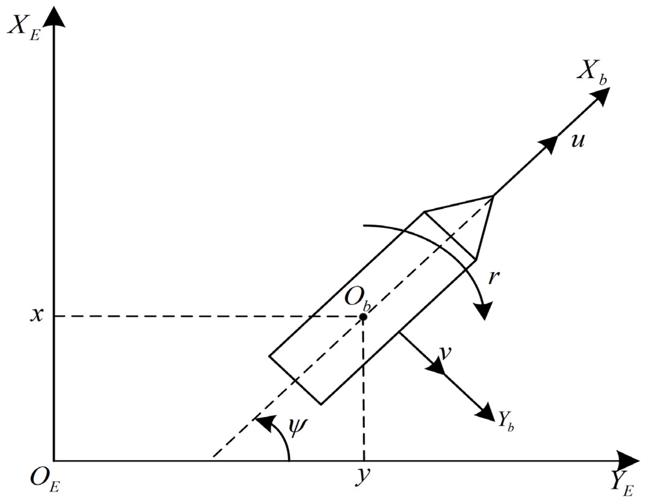
2.1. Underactuated Unmanned Surface Vessel Mathematical Motion Model

The full dynamic model of underactuated USVs has 6-DOF, namely, surge, sway, heave, roll, pitch, and yaw, respectively. Since, in most applications, only the horizontal motions of the USVs are of concern, the heave, roll, and pitch can be neglected. In this study, the USV model parameters are assumed to be known, but the external environmental disturbances are unknown. A 3-DOF mathematical model is established for the USVs, and the surge motion controller and yaw motion controller are designed as inputs to control the motion of the USVs. The following assumptions are made to design the controller.

Assumption 1.

The underactuated USV has a uniform mass distribution and a left–right symmetry, with the center of gravity located at the origin of the coordinate system.

Assumption 2.

The reference trajectory $\left(x_d,y_d\right)$ of the USV is smooth and has continuous first and second-order derivatives [39].

Definitions of the Earth-fixed and Body-fixed coordinate systems are shown in Figure 1:

In Figure 1, $O_E{X}_E{Y}_E$ is the Earth-fixed coordinate system, $O_E$ is the origin, $O_E{X}_E$ is the north direction, $O_E{Y}_E$ is the east direction, $O_b{X}_b{Y}_b$ is the Body-fixed coordinate frame, $O_b$ is the center of gravity of the USV, $O_b{X}_b$ directs to the bow, and $O_b{Y}_b$ points to the starboard.

$\left(x,y\right)$ represents the actual position of the USVs, $\psi \in \left(0,2\pi \right)$ is the heading angle of the USV, and $u$, $v$, and $r$ denote the surge velocity, the sway velocity, and the yaw velocity of the USV, respectively. Therefore, the 3-DOF mathematical model of the underactuated USV can be described as

$$\dot{\eta }=J\left(\psi \right)\upsilon$$

(1)

$$M\dot{\upsilon }=-C\left(\upsilon \right)\upsilon -D\upsilon +\tau +{\tau }_d$$

(2)

where Equations (1) and (2) are the kinematic and dynamic models of the USV, respectively. $\eta ={\left[x,y,\psi \right]}^T$ is the position vector of the USV; $\upsilon ={\left[u,v,r\right]}^T$ the velocity vector of the USV, $J\left(\psi \right)=\left[\begin{array}{ccc}\cos \psi & -\sin \psi & 0\\ \sin \psi & \cos \psi & 0\\ 0& 0& 1\end{array}\right]$ is the transformation matrix, which satisfies $J^{-1}\left(\psi \right)=J^T\left(\psi \right)$; $M=\left[\begin{array}{ccc}{m}_{11}& 0& 0\\ 0& m_{22}& 0\\ 0& 0& m_{33}\end{array}\right]$ is the inertia matrix, $C\left(\upsilon \right)=\left[\begin{array}{ccc}0& 0& -m_{22}v\\ 0& 0& m_{11}u\\ m_{22}v& -m_{11}u& 0\end{array}\right]$ the Coriolis matrix; $D=\left[\begin{array}{ccc}{d}_{11}& 0& 0\\ 0& d_{22}& 0\\ 0& 0& d_{33}\end{array}\right]$ is the hydrodynamic damping matrix; $\tau ={\left[{\tau }_u,{\tau }_v,{\tau }_r\right]}^T$ is the control input, and ${\tau }_u$ and ${\tau }_r$ is the surge motion controller and yaw motion controller of the USV, respectively. Since the USV used in this study is an underactuated system, ${\tau }_v=0$. ${\tau }_d={\left[{\tau }_{du},{\tau }_{dv},{\tau }_{dr}\right]}^T$ is used to denote unknown time-varying disturbances from the external environment, among them, $m_{11}=m+X_{\dot{u}}$, $m_{22}=m+Y_{\dot{v}}$, $m_{33}=I_z+N_{\dot{r}}$, $d_{11}=-X_u$, $d_{22}=-Y_v$, $d_{33}=-N_r$. $m$ represents the mass of USV, $I_z$ represents the moment of inertia about axis $z$, and the other parameters are hydrodynamic coefficients. Therefore, combining the kinematic and dynamic models of underactuated USV yields

$$\left\{\begin{array}{l}\dot{x}=u\cos \left(\psi \right)-v\sin \left(\psi \right)\\ \dot{y}=u\sin \left(\psi \right)+v\cos \left(\psi \right)\\ \dot{\psi }=r\\ \dot{u}=\left(m_{22}vr-d_{11}u+{\tau }_u+{\tau }_{du}\right)/m_{11}\\ \dot{v}=\left(-m_{11}ur-d_{22}v+{\tau }_{dv}\right)/m_{22}\\ \dot{r}=\left(\left(m_{11}-m_{22}\right)uv-d_{33}r+{\tau }_r+{\tau }_{dr}\right)/m_{33}\end{array}\right.$$

(3)

2.2. Overview of Biologically Inspired Neural Network

BINN refers to a series of optimization algorithm models formed by scholars inspired by some behaviors or intrinsic nature of organisms. It is inspired by the process of the occurrence and transfer of bioelectrical signals between neurons. In recent years, BINN has been widely used in trajectory tracking, path planning, and formation control due to its advantages in optimizing performance, handling unmodeled dynamics, suppressing input saturation, and controlling speed jumps. The mathematic model of BINN takes the form [40]

$$\frac{d^{2}V}{d{t}^2}=K\left\{\frac{dV}{dt}+\frac{1}{C_m}\left[g_k{n}^4\left(V-V_K\right)+g_{Na}{m}^{3}h\left(V-V_{Na}\right)+g_l\left(V-V_l\right)\right]\right\}$$

(4)

where $V$ is the value of the potential of the cell membrane; $V_{Na}$, $V_K$, $V_l$ are the potentials generated at the cell membrane by $N{a}^{+}$, $K^{+}$ and the resting potential, respectively; $g_{Na}$, $g_K$, $g_l$ is the conductance generated by $N{a}^{+}$, $K^{+}$ and passive channels, respectively; $C_m$ is the cell membrane capacitance; $K$ is a design parameter that is positive; $n$, $m$, and $h$ are parameters of the ionic activity state in the cell membrane.

Simplifying Equation (4) based on the change in cell membrane potential, the following model can be obtained:

$$C_m\frac{dV}{dt}=g_K\left(V_K-V\right)+g_{Na}\left(V_{Na}-V\right)+g_l\left(V_l-V\right)$$

(5)

Let some coefficients in Equation (5) be constants [41] denoted as $C_m=1$, $V_l-V=-X_i$, $V_{Na}-V_l=B$, $V_l-V_K=D$, $g_l=A_i$, $g_{Na}=S_i^L$, $g_K=S_i^H$, it can be obtained that

$$\frac{d{X}_i}{dt}=-A_i{X}_i+\left(B_i-X_i\right)S_i^H-\left(D_i+X_i\right)S_i^L$$

(6)

where $A_i$ is the decay rate of the potential change; $B_i$ and $D_i$ are the upper and lower bounds of the output potential, respectively; $S_i^H$ and $S_i^L$ are the excitatory and inhibitory. The stability and boundedness of the algorithm and output have been rigorously demonstrated [41], and the BINN algorithm used in this study was obtained using $f\left(\zeta \right)=\max \left\{\zeta ,0\right\}$ instead of $S_i^H$, $g\left(\zeta \right)=\max \left\{-\zeta ,0\right\}$ replace $S_i^L$:

$$\frac{d{X}_i}{dt}=-A_i{X}_i+\left(B_i-X_i\right)f\left(\zeta \right)-\left(D_i+X_i\right)g\left(\zeta \right)$$

(7)

The objective of this study is to design a BINN-based NTSM control strategy for the problem of thruster input saturation of USV, which enables the suppression of input saturation, facilitates the observation and compensation of disturbances and satisfies the stability requirements.

3. Controller Design and Stability Analysis

In this section, an NTSM controller using BINN is designed to realize the trajectory tracking control, and the structure of the whole design scheme is shown in Figure 2.

3.1. Virtual Control Law Design

The purpose of trajectory tracking control of USVs is typically to continuously adjust the controller based on positional error information, ultimately making the position error calm down to zero. To achieve this, the Lyapunov function must be constructed based on the positional error equation, and the virtual control law must be designed to satisfy the Lyapunov stability theory and enable trajectory tracking control. Therefore, the position tracking error $x_e$, $y_e$ is defined as

$$\left\{\begin{array}{l}{x}_e=x-x_d\\ y_e=y-y_d\end{array}\right.$$

(8)

where $x_d$ and $y_d$ are the reference position of USV; and $x$ and $y$ is the actual position of USV.

It can be derived from Equations (8) and (3) that

$$\left\{\begin{array}{c}{\dot{x}}_e=u\cos \left(\psi \right)-v\sin \left(\psi \right)-{\dot{x}}_d\\ {\dot{y}}_e=u\sin \left(\psi \right)+v\cos \left(\psi \right)-{\dot{y}}_d\end{array}\right.$$

(9)

Define the vertical velocity error and lateral velocity error of the USV as follows:

$$\left\{\begin{array}{l}{u}_e=u-{\alpha }_u\\ v_e=v-{\alpha }_v\end{array}\right.$$

(10)

where ${\alpha }_u$ is the designed vertical virtual control law and ${\alpha }_v$ the designed lateral virtual control law. Combining Equations (9) and (10) gives the following equations:

$$\left\{\begin{array}{c}{\alpha }_u={\dot{x}}_d\cos \left(\psi \right)+{\dot{y}}_d\sin \left(\psi \right)-\frac{k_1{x}_e}{\sqrt{x_e^2+y_e^2+D}}\cos \left(\psi \right)-\frac{k_2{y}_e}{\sqrt{x_e^2+y_e^2+D}}\sin \left(\psi \right)\\ {\alpha }_v=-{\dot{x}}_d\sin \left(\psi \right)+{\dot{y}}_d\cos \left(\psi \right)+\frac{k_1{x}_e}{\sqrt{x_e^2+y_e^2+D}}\sin \left(\psi \right)-\frac{k_2{y}_e}{\sqrt{x_e^2+y_e^2+D}}\cos \left(\psi \right)\end{array}\right.$$

(11)

where $k_1>0$, $k_2>0$, $D>0$ are designed constants. Substituting Equations (10) and (11) into Equation (9):

$$\left\{\begin{array}{c}{\dot{x}}_e=\left(u-{\alpha }_u\right)\cos \left(\psi \right)-\left(v-{\alpha }_v\right)\sin \left(\psi \right)-\frac{k_1{x}_e}{\sqrt{x_e^2+y_e^2+D}}\\ {\dot{y}}_e=\left(u-{\alpha }_u\right)\sin \left(\psi \right)+\left(v-{\alpha }_v\right)\cos \left(\psi \right)-\frac{k_2{y}_e}{\sqrt{x_e^2+y_e^2+D}}\end{array}\right.$$

(12)

where $\mathsf{\Lambda }=\sqrt{{\mathrm{x}}_e^2+y_e^2+D}$. For $u-{\alpha }_u=0$ and $v-{\alpha }_v=0$, Equation (12) can be expressed as

$$\left\{\begin{array}{c}{\dot{x}}_e=-\frac{k_1{x}_e}{\mathsf{\Lambda }}\\ {\dot{y}}_e=-\frac{k_2{y}_e}{\mathsf{\Lambda }}\end{array}\right.$$

(13)

Consider the Lyapunov function:

$$V_1=\frac{1}{2}{x}_e^2+\frac{1}{2}{y}_e^2$$

(14)

The derivative of Equation (14) is given by

$${\dot{V}}_1=x_e{\dot{x}}_e+y_e{\dot{y}}_e=\frac{-k_1{x}_e^2-k_2{y}_e^2}{\mathsf{\Lambda }}$$

(15)

Following Equation (15) and Lyapunov stability theory, it can be obtained that when $\underset{t\to \infty }{\lim }{\dot{V}}_1\le 0$, the position errors $x_e$ and $y_e$ of the USV converge to zero asymptotically, and the system is stabilized. It is shown that when the velocity error converges to zero, the position error also converges to zero.

3.2. Nonlinear Extended State Observer Design

In the actual navigation process, the underactuated USV will be affected by disturbances from the external environment. Considering that the disturbances are non-negligible and cannot be directly measured, a NESO is introduced into the control system to estimate the unknown disturbances and to improve the ability to resist disturbances.

According to the USV mathematical model Equation (1), it can be obtained that

$$\begin{array}{ll}\ddot{\eta }& =\dot{J}\left(\psi \right)\upsilon +J\left(\psi \right)\dot{\upsilon }\\ & =\dot{J}\left(\psi \right)\upsilon +J\left(\psi \right)M^{-1}\left(-C\left(\upsilon \right)\upsilon -D\upsilon +\tau +{\tau }_d\right)\\ & =\dot{J}\left(\psi \right)\upsilon +J\left(\psi \right)M^{-1}\left(-C\left(\upsilon \right)\upsilon -D\upsilon \right)+J\left(\psi \right)M^{-1}\tau +J\left(\psi \right)M^{-1}{\tau }_d\\ & =F_1+F_2\tau +d\end{array}$$

(16)

where $F_1=\dot{J}\left(\psi \right)\upsilon +J\left(\psi \right)M^{-1}\left(-C\left(\upsilon \right)\upsilon -D\upsilon \right)$, $F_2=J\left(\psi \right)M^{-1}$, $d=J\left(\psi \right)M^{-1}{\tau }_d$.

Construct a NESO in the following form [42]:

$$\left\{\begin{array}{l}{\dot{\widehat{z}}}_1={\widehat{z}}_2+{\gamma }_1\left(z_1-{\widehat{z}}_1\right)\\ {\dot{\widehat{z}}}_2={\widehat{z}}_3+F_2\tau +{\widehat{F}}_1+{\gamma }_2{\chi }_2\\ {\dot{\widehat{z}}}_3={\gamma }_3{\chi }_3\end{array}\right.$$

(17)

where ${\widehat{z}}_1$ is the estimation of the position vector $\eta$ of the USV, ${\widehat{z}}_2$ the estimation of $\dot{\eta }$, ${\gamma }_i\left(i=1,2,3\right)>0$ denotes the control gain of the NESO, ${\widehat{z}}_3$ the estimation of the part with the disturbance term, ${\widehat{F}}_1=\dot{J}\left(\psi \right)\widehat{\upsilon }+J\left(\psi \right)M^{-1}\left(-C\left(\upsilon \right)\widehat{\upsilon }-D\widehat{\upsilon }\right)$ the observation of $F_1$. The observation error is defined as $e_1=z_1-{\widehat{z}}_1$, $e_2=z_2-{\widehat{z}}_2$, $e_3=z_3-{\widehat{z}}_3$.

For vector ${\chi }_i={\mathrm{fal}}_i\left(e_1,{\alpha }_i,{\delta }_i\right),\left(i=1,2\right)$, define

$${\mathrm{fal}}_i\left(e_1,{\alpha }_i,{\delta }_i\right)=\left\{\begin{array}{l}{\left|e_1\right|}^{{\alpha }_i}\mathrm{sign}\left(e_1\right),\left|e_1\right|>{\delta }_i\\ \frac{e_1}{{\delta }_i^{1-{\alpha }_i}} ,\left|e_1\right|\le {\delta }_i\end{array}\right.$$

(18)

where ${\alpha }_i\in \left(0,1\right)$, ${\delta }_i>0\left(i=1,2\right)$ is a design parameter of small value.

Combining Equations (1), (16), and (17), the error dynamic equations for the NESO can be obtained:

$$\left\{\begin{array}{l}{\dot{e}}_1=e_2-{\gamma }_1{e}_1\\ {\dot{e}}_2=e_3-{\gamma }_2{\chi }_2+{\tilde{F}}_1\\ {\dot{e}}_3=-{\gamma }_3{\chi }_3+\dot{d}\end{array}\right.$$

(19)

where ${\tilde{F}}_1=F_1-{\widehat{F}}_1$, $\left|\dot{d}\right|\le H$, $H>0$.

To analyze the stability of the NESO, the error vector is defined as $e={\left[e_1,e_2,e_3\right]}^T\in R^9$. The following expression can be derived:

$$\dot{e}=Ae+B$$

(20)

where $A=\left[\begin{array}{ccc}-{\gamma }_1& I_3& 0_3\\ -{\gamma }_2& 0_3& I_3\\ -{\gamma }_3& 0_3& 0_3\end{array}\right]$, $B=\left[\begin{array}{c}{0}_3\\ {\tilde{F}}_1\\ H\end{array}\right]$.

The eigenvalue matrix of $A$ is

$$\left|sI-A\right|=\left[\begin{array}{ccc}s+{\gamma }_1& -I_3& 0_3\\ {\gamma }_2& s& -I_3\\ {\gamma }_3& 0_3& s\end{array}\right]$$

(21)

The characteristic polynomial of Equation (21) is

$$s^3+{\beta }_1{s}^2+{\beta }_{2}s+{\beta }_3=0$$

(22)

According to Lyapunov stability theory, for any given positive definite matrices $Q$ and $P$, the following Lyapunov equation is satisfied.

$$A^{T}P+PA+Q=0$$

(23)

Design the Lyapunov function:

$$V_2=e^{T}Pe$$

(24)

The time derivative of Equation (24):

$$\begin{array}{ll}{\dot{V}}_2& ={\dot{e}}^{T}Pe+e^{T}P\dot{e}\\ & ={\left(Ae+B\right)}^{T}Pe+e^{T}P\left(Ae+B\right)\\ & =e^T\left(A^{T}P+PA\right)e+2e^{T}PB\\ & \le e^T\left(A^{T}P+PA\right)e+2‖e‖P{\mu }_1‖e‖\\ & \le -e^{T}Qe+2{\mu }_1‖P‖{‖e‖}^2\end{array}$$

(25)

where ${\mu }_1>0$. The quadratic inequality holds: ${\lambda }_{\min }\left(Q\right){‖e‖}^2\le e^{T}Qe\le {\lambda }_{\max }\left(Q\right){‖e‖}^2$, ${\lambda }_{\min }\left(Q\right)$ and ${\lambda }_{\max }\left(Q\right)$ are the minimum and maximum eigenvalue of the matrix $Q$, which satisfied ${\gamma }_i{\left|e\right|}^{{\alpha }_i}\le {‖e‖}^2\le V_2/{\lambda }_{\min }\left(Q\right)$.

Then, Equation (25) can be written as

$$\begin{array}{ll}{\dot{V}}_2& \le -{\lambda }_{\min }\left(Q\right){‖e‖}^2+2{\mu }_1‖P‖{‖e‖}^2\\ & \le -\left({\lambda }_{\min }\left(Q\right)-2{\mu }_1‖P‖\right){‖e‖}^2\\ & \le -{\mu }_2{V}_2/{\lambda }_{\min }\left(Q\right)\end{array}$$

(26)

where ${\mu }_2={\lambda }_{\min }\left(Q\right)-2{\mu }_1‖P‖>0$, so that ${\dot{V}}_2<0$, the observer error system is stable and the error is bounded.

Therefore, the values of the disturbance observed by NESO are ${\widehat{\tau }}_d={\left[{\widehat{\tau }}_{du},{\widehat{\tau }}_{dv},{\widehat{\tau }}_{dr}\right]}^T=J^{-1}\left(\psi \right)M\widehat{d}$.

3.3. Controller Design

3.3.1. Surge Motion Controller Design Using Biologically Inspired Neural Network

Based on the vertical velocity error $u_e$, the following NTSM surface can be designed:

$$s_1={\displaystyle {\int }_{t_0}^t{u}_{e}dt}+{\beta }_1{\left(u_e\right)}^{p_1/q_1}$$

(27)

where ${\beta }_1>0$ is a design constant; $p_1$ and $q_1$ the odd positive integers that satisfy $p_1>q_1$.

The derivative of $s_1$ with respect to time $t$ is

$${\dot{s}}_1=u_e+{\beta }_1\frac{p_1}{q_1}{\left(u_e\right)}^{p_1/q_1-1}\left(\frac{m_{22}}{m_{11}}vr-\frac{d_{11}}{m_{11}}u+\frac{1}{m_{11}}{\tau }_u+\frac{1}{m_{11}}{\tau }_{du}-{\dot{\alpha }}_u\right)$$

(28)

To simplify the design of the controller, the designed vertical velocity control law ${\alpha }_u$ is incorporated into the BINN, yielding the following expression:

$$\begin{array}{ll}{\dot{X}}_u& =-A_1{X}_u+\left(B_1-X_u\right)f\left({\alpha }_u\right)-\left(D_1+X_u\right)g\left({\alpha }_u\right)\\ & =-\left[A_1+f\left({\alpha }_u\right)+g\left({\alpha }_u\right)\right]X_u+B_{1}f\left({\alpha }_u\right)-D_{1}g\left({\alpha }_u\right)\end{array}$$

(29)

After a transformation of the BINN ${\dot{\alpha }}_u={\dot{X}}_u$, Equation (28) can be written as

$${\dot{s}}_1=u_e+{\beta }_1\frac{p_1}{q_1}{\left(u_e\right)}^{p_1/q_1-1}\left(\left(m_{22}vr-d_{11}u+{\tau }_u+{\tau }_{du}\right)/m_{11}-{\dot{X}}_u\right)$$

(30)

To achieve a kinematic stabilization of the USV system, a surge motion controller ${\tau }_u$ using BINN is designed in the following form:

$${\tau }_{\mathrm{u}}=-m_{22}vr+d_{11}u+m_{11}{\dot{X}}_u-m_{11}\frac{1}{{\beta }_1}\frac{q_1}{p_1}{\left(u_e\right)}^{2-p_1/q_1}-{\lambda }_1\mathrm{sat}\left(s_1\right)-{\widehat{\tau }}_{du}$$

(31)

where ${\widehat{\tau }}_{du}$ represents the disturbance value observed by NESO in the surge direction, ${\lambda }_1>0$ is a design constant, and $\delta$ is a small positive value. In order to improve the issue of chattering in the traditional SMC, the symbolic function is replaced with the function $\mathrm{sat}\left(x\right)$, and a controller is designed. The expression of function $\mathrm{sat}\left(x\right)$ used in this subsection is as follows:

$$\mathrm{sat}(x)=\left\{\begin{array}{r}\hfill 1,x>\delta \\ \hfill x/\delta , \left|x\right|\le \delta \\ \hfill -1,x<-\delta \end{array}\right.$$

(32)

Consider the Lyapunov function:

$$V_3=\frac{1}{2}{m}_{11}{s}_1^2$$

(33)

The derivative of Equation (33) is given by

$$\begin{array}{ll}{\dot{V}}_3& =m_{11}{s}_1{\dot{s}}_1\\ & =m_{11}{s}_1\left(u_e+{\beta }_1\frac{p_1}{q_1}{\left(u_e\right)}^{p_1/q_1-1}\left(\left(m_{22}vr-d_{11}u+{\tau }_u+{\tau }_{du}\right)/m_{11}-{\dot{X}}_u\right)\right)\\ & ={\beta }_1\frac{p_1}{q_1}{\left(u_e\right)}^{p_1/q_1-1}{s}_1\left(-{\lambda }_{1}sat\left(s_1\right)+{\tau }_{du}-{\widehat{\tau }}_{du}\right)\\ & ={\beta }_1\frac{p_1}{q_1}{\left(u_e\right)}^{p_1/q_1-1}{s}_1\left(-{\lambda }_{1}sat\left(s_1\right)\right)+{\beta }_1\frac{p_1}{q_1}{\left(u_e\right)}^{p_1/q_1-1}{s}_1{\tilde{\tau }}_{du}\end{array}$$

(34)

where ${\tilde{\tau }}_{du}={\tau }_{du}-{\widehat{\tau }}_{du}$ is the disturbance error, and ${\beta }_1\frac{p_1}{q_1}{\left(u_e\right)}^{p_1/q_1-1}\ge 0$.

It follows Equation (26) that the observation error of the NESO converges, and errors are bounded so that ${\tilde{\tau }}_{du}$ is stable and converges to zero.

Therefore, Equation (34) can be written as

$${\dot{V}}_3\le -{\lambda }_1{\beta }_1\frac{p_1}{q_1}{\left(u_e\right)}^{p_1/q_1-1}\left|s_1\right|$$

(35)

3.3.2. Design of Yaw Motion Controller Using Biologically Inspired Neural Network

Since the USV has no thrusters in the transverse direction, the following NTSM is designed to allow control input ${\tau }_r$ to occur in the ${\dot{s}}_2$

$$s_2=v_e+{\beta }_2{\left({\dot{v}}_e\right)}^{p_2/q_2}$$

(36)

where ${\beta }_2>0$ is design constant, $p_2$ and $q_2$ are odd positive integers satisfying $p_2>q_2$.

The derivative of $s_2$ with respect to time $t$ is

$${\dot{s}}_2={\dot{v}}_e+{\beta }_2\frac{p_2}{q_2}{\ddot{v}}_e{\left({\dot{v}}_e\right)}^{p_2/q_2-1}$$

(37)

It can be derived from Equation (10), that ${\dot{v}}_e=\dot{v}-{\dot{\alpha }}_v$, ${\ddot{v}}_e=\ddot{v}-{\ddot{\alpha }}_v$. Define $\omega$ as

$$\begin{array}{ll}\omega & =\left[{\ddot{y}}_d-k_2\left({\mathsf{\Lambda }}^{-1}-{\mathsf{\Lambda }}^{-3}{y}_e^2\right){\dot{y}}_e+k_1{\mathsf{\Lambda }}^{-3}{x}_e{y}_e{\dot{x}}_e\right]\cos (\psi )\\ & -\left[{\ddot{x}}_d-k_1\left({\mathsf{\Lambda }}^{-1}-{\mathsf{\Lambda }}^{-3}{x}_e^2\right){\dot{x}}_e+k_2{\mathsf{\Lambda }}^{-3}{x}_e{y}_e{\dot{y}}_e\right]\sin (\psi )\end{array}$$

(38)

Then, ${\dot{\alpha }}_v=-r{\alpha }_u+\omega$, so that ${\ddot{\alpha }}_v=-\dot{r}{\alpha }_u-r{\dot{\alpha }}_u+\dot{\omega }$. To simplify the derivation process, by substituting $\omega$ into the BINN, the following expression is obtained:

$${\dot{X}}_v=-A_2{X}_v+\left(B_2-X_v\right)f\left(\omega \right)-\left(D_2+X_v\right)g\left(\omega \right)$$

(39)

From Equation (3), the differential equation of $\dot{v}$ can be obtained:

$$\ddot{v}=\left[\begin{array}{c}-d_{22}{m}_{33}\dot{v}+m_{33}{\dot{\tau }}_{dv}-m_{11}{m}_{33}\dot{u}r-m_{11}u{\tau }_r-m_{11}u{\tau }_{dr}\\ +m_{11}{d}_{33}ur+m_{11}\left(m_{22}-m_{11}\right)u^{2}v\end{array}\right]/m_{22}{m}_{33}$$

(40)

Combining Equations (37), (39), and (40) yields

$${\dot{s}}_2=\frac{{\beta }_2{p}_2{\left({\dot{v}}_e\right)}^{p_2/q_2-1}\left[\left(m_{22}{\alpha }_u-m_{11}u\right)\left({\tau }_r+{\tau }_{dr}\right)+h\right]}{q_2{m}_{22}{m}_{33}}$$

(41)

and

$$\begin{array}{ll}h& =m_{22}{\alpha }_u\left[\left(m_{11}-m_{22}\right)uv-d_{33}r\right]+m_{22}{m}_{33}\left[r{\dot{X}}_u-{\dot{X}}_v+{\beta }_2\frac{q_2}{p_2}{\left({\dot{v}}_e\right)}^{2-p_2/q_2}\right]-d_{22}{m}_{33}\dot{v}\\ & -m_{11}{m}_{33}\dot{u}r+m_{11}{d}_{33}ur+m_{11}\left(m_{22}-m_{11}\right)u^{2}v+m_{33}{\dot{\widehat{\tau }}}_{dv}\end{array}$$

(42)

where ${\dot{\widehat{\tau }}}_{dv}$ is the derivative of the disturbance value ${\widehat{\tau }}_{dv}$ in the sway direction observed by NESO.

Design the yaw motion control law as follows:

$${\tau }_r=-\frac{h}{b}-{\lambda }_2\mathrm{sat}\left(s_2\right)-{\widehat{\tau }}_{dr}$$

(43)

where ${\widehat{\tau }}_{dr}$ is the disturbance value in the direction of the yaw observed by NESO, $b=m_{22}{\alpha }_u-m_{11}u$, ${\lambda }_2>0$ is a design constant, and the $\mathrm{sat}(x)$ function is chosen as shown in Equation (32).

Consider the Lyapunov function:

$$V_4=\frac{1}{2}{m}_{22}{m}_{33}{s}_2^2$$

(44)

The derivative of Equation (44) is given by

$$\begin{array}{ll}{\dot{V}}_4& =m_{22}{m}_{33}{s}_2{\dot{s}}_2\\ & ={\beta }_2\frac{p_2}{q_2}{\left({\dot{v}}_e\right)}^{p_2/q_2-1}{s}_2\left(-{\lambda }_2\mathrm{sat}(s_2)+{\tau }_{dr}-{\widehat{\tau }}_{dr}\right)\\ & ={\beta }_2\frac{p_2}{q_2}{\left({\dot{v}}_e\right)}^{p_2/q_2-1}{s}_2\left(-{\lambda }_2\mathrm{sat}\left(s_2\right)\right)+{\beta }_2\frac{p_2}{q_2}{\left({\dot{v}}_e\right)}^{p_2/q_2-1}{s}_2{\tilde{\tau }}_{dr}\end{array}$$

(45)

It follows Equation (26) that the observation error of the NESO converges, and errors are bounded so that ${\tilde{\tau }}_{dr}$ is stable and converges to zero.

Therefore, Equation (45) can be written as

$${\dot{V}}_4\le -{\lambda }_2{\beta }_2\frac{p_2}{q_2}{\left({\dot{v}}_e\right)}^{p_2/q_2-1}\left|s_2\right|$$

(46)

3.4. Stability Analysis

In this subsection, the proposed control method is used for the trajectory tracking control of a USV, and the structure of the control strategy is shown in Figure 2. The stability analysis is then given by the following theorem.

The trajectory tracking control problem of an underactuated USV with unknown environmental disturbances is described in Equations (1) and (2). The selection of appropriate parameters $k_i\left(i=1,2\right)$, ${\beta }_i\left(i=1,2\right)$, ${\lambda }_i\left(i=1,2\right)$, $p_i\left(i=1,2\right)$, $q_i\left(i=1,2\right)$, ${\alpha }_i\left(i=1,2\right)$, and ${\gamma }_i\left(i=1,2,3\right)$ is crucial for designing the virtual control law, controller, and NESO. The choice of these parameters can ensure that the system outputs track the given reference signals and ensure that all the variables in the closed-loop system remain consistent and ultimately bounded.

Consider the Lyapunov function:

$$V_5=V_3+V_4$$

(47)

Derivation of the Equation (47) gives

$$\begin{array}{ll}{\dot{V}}_5& ={\dot{V}}_3+{\dot{V}}_4\\ & \le -{\lambda }_1{\beta }_1\frac{p_1}{q_1}{\left(u_e\right)}^{p_1/q_1-1}\left|s_1\right|-{\lambda }_2{\beta }_2\frac{p_2}{q_2}{\left({\dot{v}}_e\right)}^{p_2/q_2-1}\left|s_2\right|\\ & \le -C_1\sqrt{V_3}-C_2\sqrt{V_4}\le -C\sqrt{V_5}\end{array}$$

(48)

where $C_1=\sqrt{2/m_{11}}{\lambda }_1{\beta }_1\frac{p_1}{q_1}{\left(u_e\right)}^{p_1/q_1-1}$, $C_2=\sqrt{2/m_{22}{m}_{33}}{\lambda }_2{\beta }_2\frac{p_2}{q_2}{\left({\dot{v}}_e\right)}^{p_2/q_2-1}$, $C=\min \left\{C_1,C_2\right\}$.

It follows from Equation (48) that $\underset{t\to \infty }{\lim }{\dot{V}}_5\left(t\right)\le 0$, according to the Lyapunov stability theory criterion in [43], shows that the closed-loop system of trajectory tracking control for the underactuated USV is stable and the error converges in finite time.

4. Simulation Studies

In this section, experimental simulations are conducted to verify the effectiveness of the proposed controllers in handling input saturation. Additionally, the stability of the controllers in the presence of unknown external disturbances is also evaluated during these experiments. The long-range patrol vessel “BAY CLASS” [44] is used for the simulations. The length of the vessel is $38 \mathrm{m}$, the mass of the vessel is $m=1.18\times {10}^5\mathrm{kg}$, and the other parameters of the vessel are shown in

Table 1. USV model parameters.

Parameter	Value	Units
$m_{11}$	$1.2\times {10}^5$	$\mathrm{kg}$
$m_{22}$	$1.779\times {10}^5$	$\mathrm{kg}$
$m_{33}$	$6.36\times {10}^7$	$\mathrm{kg}\cdot {\mathrm{m}}^2$
$d_{11}$	$2.15\times {10}^4$	$\mathrm{kg}/\mathrm{s}$
$d_{22}$	$1.47\times {10}^5$	$\mathrm{kg}/\mathrm{s}$
$d_{33}$	$8.02\times {10}^6$	$\mathrm{kg}\cdot {\mathrm{m}}^2/\mathrm{s}$

. The virtual control law, NESO, and controllers in the design process are modeled using the Simulink simulation tool in MATLAB. The version number of MATLAB is 9.8.0.1323502 (R2020a), and the solver ode45 is chosen with variable step size. All the simulations are conducted on a personal computer equipped with an Intel(R) Core(TM) i5-6300 HQ CPU @ 2.30 GHz (Intel Corporation, Santa Clara, CA, USA)and a 16 GB Memory Stick (NVIDIA Corporation, Santa Clara, CA, USA). The work of the simulation is divided into two stages.

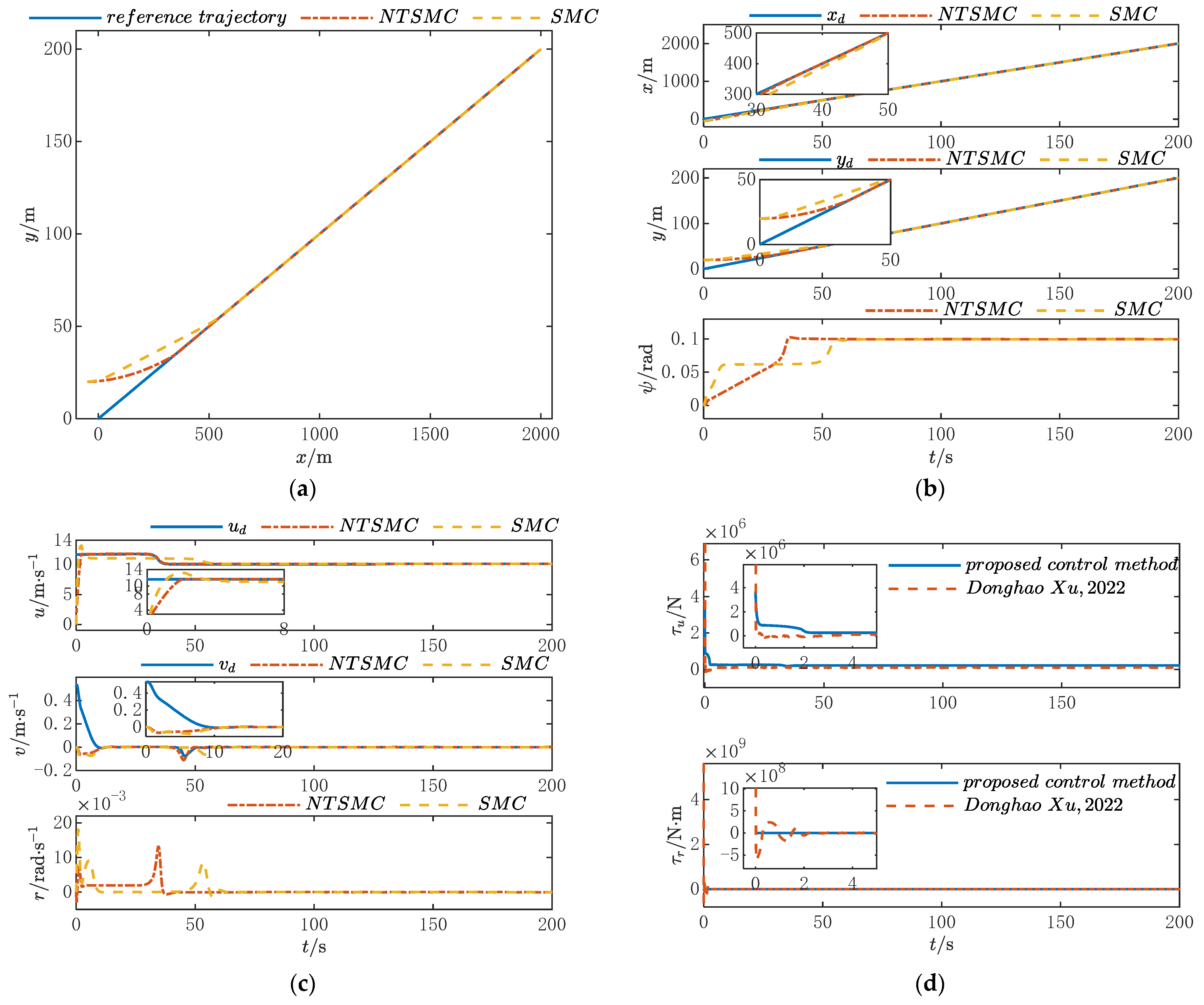
4.1. Trajectory Tracking on a Straight Path

To verify the trajectory tracking control effect of the USV on the straight path, the straight trajectory is designed as $x_d=10t$, $y_d=t$, and the slow time-varying disturbances are used to simulate the actual sea conditions with less wind, waves, and slower environmental changes during the navigation.

$$\left\{\begin{array}{l}{\tau }_{du}=1\times {10}^3\times \left(\sin 0.2t+\cos 0.5t\right)\\ {\tau }_{dv}=1\times {10}^2\times \left(\sin 0.1t\right)\\ {\tau }_{dr}=1\times {10}^4\times \left(\sin 0.5t+\cos 0.3t\right)\end{array}\right.$$

(49)

The initial positions and velocities of the USV are assumed as ${\eta }_0={\left[-50,20,0\right]}^T$ and ${\upsilon }_0={\left[0,0,0\right]}^T$. For the control method designed in this study, increasing the control gain improves the steady-state performance of the system, but it slows down the convergence speed of the error. Therefore, to achieve faster convergence speed and better steady-state performance, the virtual control gains ($k_1$ and $k_2$) are generally chosen to be constants around 1, the controller gains ${\lambda }_1$ and ${\lambda }_2$ are larger constants. Thus, the control parameters of the USV are selected as $k_1=k_2=1.3$, $D=5$, ${\beta }_1=5$, ${\beta }_2=1$, $p_1=p_2=5$, $q_1=q_2=3$, ${\lambda }_1=3\times {10}^4$, ${\lambda }_2=2\times {10}^4$. The relevant parameters for the BINN are $A_1=10$, $B_1=D_1=2$, $A_2=4$, $B_2=D_2=7$. The parameters for NESO are set as ${\gamma }_1=\mathrm{diag}\left(10,10,10\right)$, ${\gamma }_2=\mathrm{diag}\left(11,6,8\right)$, ${\gamma }_3=\mathrm{diag}\left(5,7,8\right)$, ${\alpha }_1=\mathrm{diag}\left(0.3,0.5,0.2\right)$, ${\alpha }_2=\mathrm{diag}\left(0.2,0.5,0.5\right)$. The simulation results are shown in Figure 3, Figure 4 and Figure 5.

The simulation results of the straight path for USV are shown in Figure 3. Figure 3a shows the trajectory tracking results for the USV, where the blue line is the reference trajectory, the red line is the actual trajectory formed by the proposed control method, and the orange line is the actual trajectory formed by the original SMC. It can be seen that the tracking speed of the proposed control method is significantly faster than that of the original SMC method. Figure 3b shows the USV in the $xy$ plane over time, which reflects the tracking situation when the trajectory changes over time. Figure 3c shows the results of velocity tracking for USV, which shows that the proposed method converges faster than the original SMC. Figure 3d shows the change curve of the control inputs. Compared with the control method used by Xu [45], the NTSM controller with the addition of a BINN has a significant suppression effect on the input saturation, and from the results, the plotted curves are rounded and smooth, and the symbolic function has been replaced with the $\mathrm{sat}\left(x\right)$ function so that the controller chattering problem is effectively solved. Figure 4 shows the position errors and the velocity errors. It can be seen that the position error and the velocity error convergence speed of the proposed method are faster than that of the original SMC and are more stable.

Figure 5 shows the observation results of NESO for the positions, velocities, and disturbances of the USV system. It can be seen that the designed NESO can accurately estimate the position and velocity information of the USV and can quickly and accurately estimate the unknown disturbances curve with accurate estimation results. Since the initial position of the USV is far from the reference position, there is some overshooting in the initial stage, but it does not affect the observation results and improves the robustness of the system. Figure 5c shows the comparison curves between the Nonlinear Disturbance Observer (NDOB) and NESO’ for disturbance observation. From the results, it can be seen that the observation speed of NDOB is slower than NESO, and there is a certain degree of hysteresis.

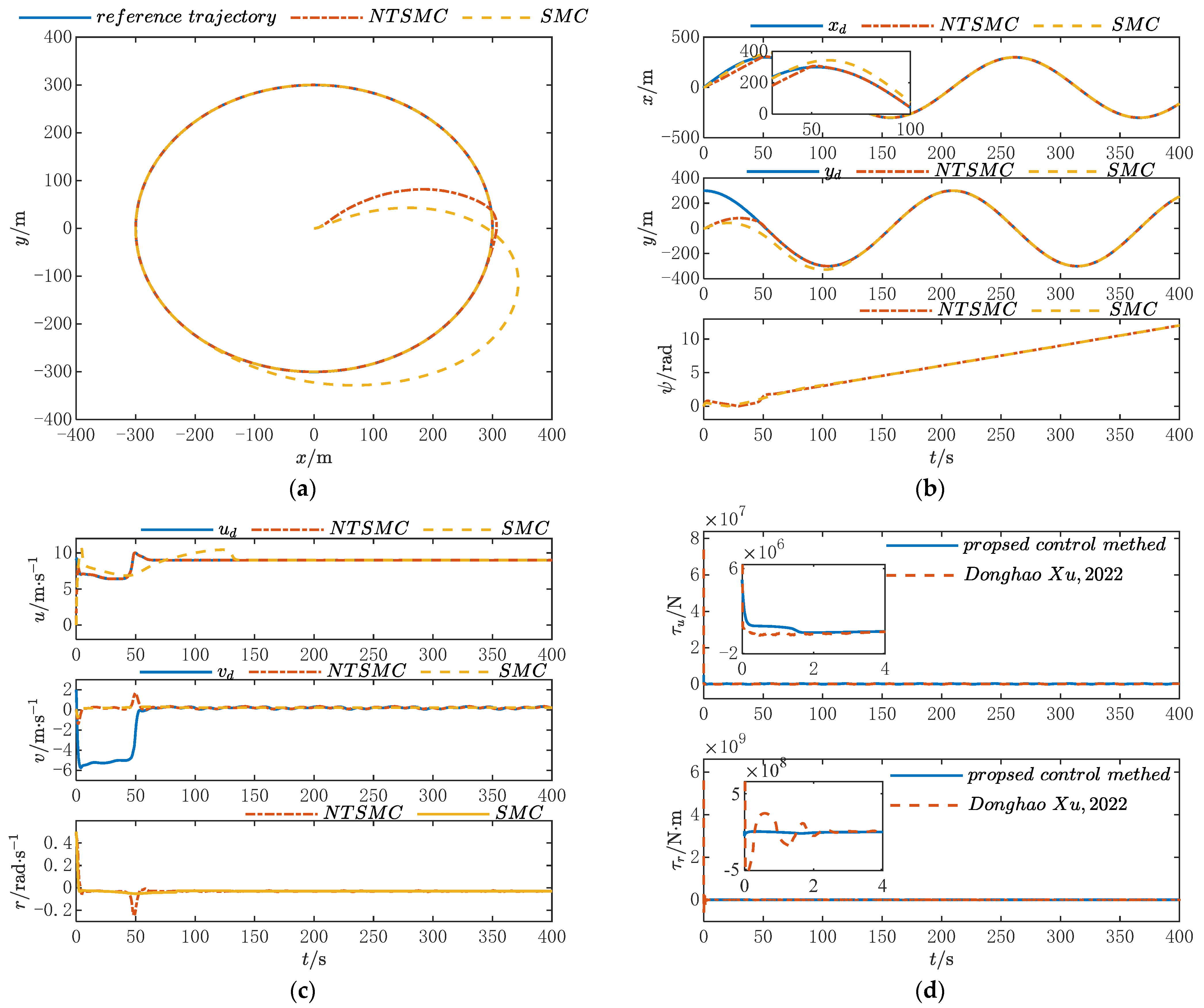
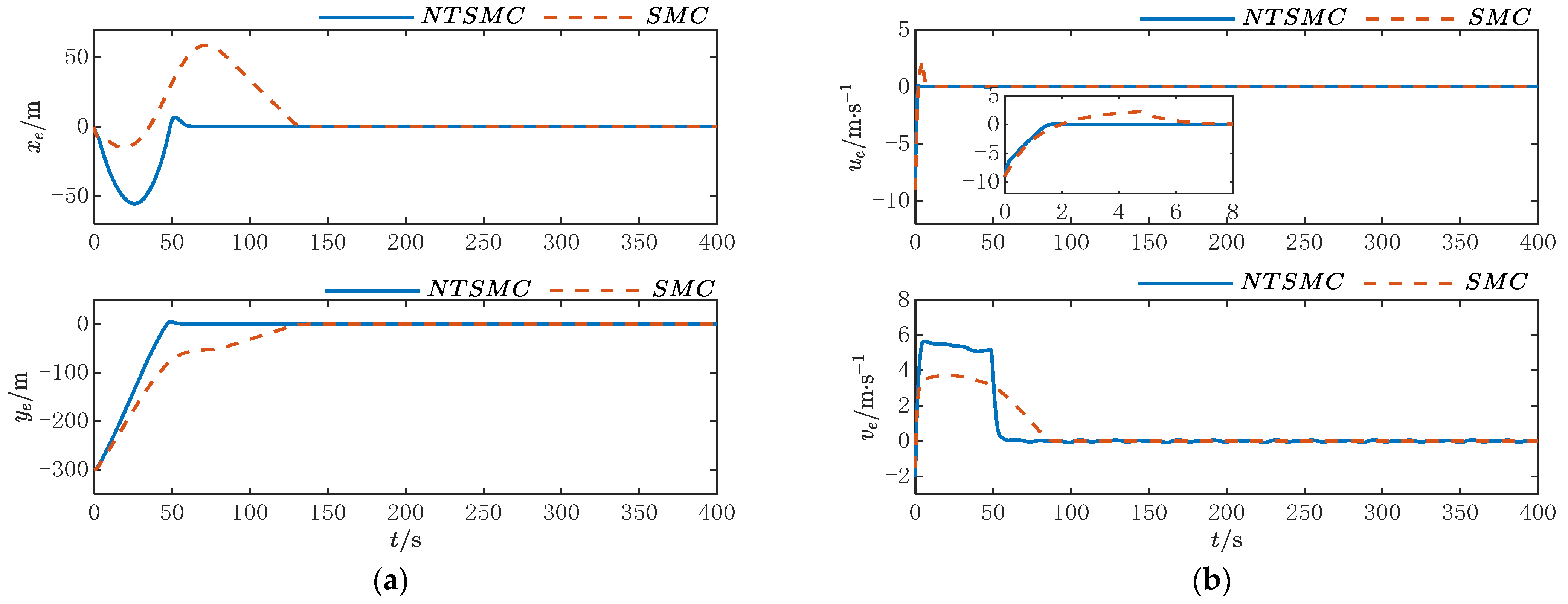
4.2. Trajectory Tracking on a Circular Path

To further verify the effectiveness of the proposed control method, the circular path is set as $x_d=300\sin \left(0.03t\right)$, $y_d=300\cos \left(0.03t\right)$, and the following strong time-varying disturbances are used to simulate the actual sea conditions with strong winds, waves, or strong environmental changes during the navigation.

$$\left\{\begin{array}{l}{\tau }_{du}=1\times {10}^5\times \left(\sin 0.2t+\cos 0.5t\right)\\ {\tau }_{dv}=1\times {10}^4\times \left(\sin 0.1t+\cos 0.4t\right)\\ {\tau }_{dr}=1\times {10}^6\times \left(\sin 0.5t+\cos 0.3t\right)\end{array}\right.$$

(50)

The initial positions and velocities of the USV are assumed as ${\eta }_0={\left[0,0,0\right]}^T$ and ${\upsilon }_0={\left[0,0,\pi /6\right]}^T$. The control parameters of the USV used are $k_1=1.6$, $k_2=2.0$, $D=10$, ${\beta }_1=5$, ${\beta }_2=10/9$, $p_1=p_2=5$, $q_1=q_2=3$, ${\lambda }_1=1\times {10}^4$, and ${\lambda }_2=1\times {10}^4$. The parameters for the BINN are $A_1=9$, $B_1=D_1=4$, and $A_2=B_2=D_2=10$. The parameters for NESO are ${\gamma }_1=\mathrm{diag}\left(15,15,15\right)$, ${\gamma }_2=\mathrm{diag}\left(11,13,8\right)$, ${\gamma }_3=\mathrm{diag}\left(15,20,20\right)$, ${\alpha }_2=\mathrm{diag}\left(0.3,0.3,0.2\right)$, and ${\alpha }_3=\mathrm{diag}\left(0.1,0.1,0.2\right)$. The simulation results are shown in Figure 6, Figure 7 and Figure 8.

Figure 6 presents the simulation results for the case of the circular path. Figure 6a shows the trajectory tracking curve. It can be seen that when the reference trajectory changes from a straight line to a curve, the designed controller can still enable the USV to track the reference trajectory. Figure 6b,c show the results for position tracking and speed tracking. Figure 6d shows the curve of changes in the control inputs.

Figure 7 shows position errors and the speed tracking errors. For the initial position of the USV far away from the reference position, the error is large at the initial stage of speed tracking, but after the USV achieves stable tracking, the speed error convergences to zero faster than the original SMC, which suggests the efficiency of the controller design.

Figure 8 shows the observation results of positions, velocities, and external disturbances information using NESO, from which it can be seen that the designed NESO can still accurately and quickly observe the strongly varying disturbances. The overshooting is also small. Figure 5c is the comparison of curves between the NDOB and NESO for disturbance observation.

5. Conclusions

This paper proposes an NTSM controller incorporating the BINN method for trajectory tracking control of underactuated USV accounting for the input saturation and the unknown external environmental disturbances. The BINN method is employed to mitigate the problem of controller input saturation, while the NESO is designed to accurately observe unknown disturbances. By utilizing the Lyapunov stability criterion, it has been demonstrated that the designed control method can stabilize the error, ensuring a bound of errors. The proposed control method is validated through simulations for two different real sea conditions. Based on the observation and analysis of the results, the following conclusions are drawn:

(1)

The design of the virtual control law simplifies the trajectory tracking problem by converting the initial large position error into a smaller velocity error and achieves USV trajectory tracking control by stabilizing the velocity error. This approach significantly reduces the complexity of control and holds great practical significance.

(2)

The BINN can effectively deal with the issue of controller input saturation during USV navigation, which enhances USV performance in terms of safety. The BINN simplifies the controller design process, resulting in faster derivation and smaller computational requirements, resulting in a smooth and bounded output system.

(3)

The proposed NTSM controllers using BINN exhibit better control performance than SMC. Furthermore, this proposed approach effectively minimizes position and velocity errors to zero within a short time, increasing the response speed of the system and improving overall accuracy.

(4)

A NESO has been designed to accurately observe the unknown environmental disturbances, the position and velocity information of the USV, and the designed NESO is verified to effectively counteract the influence of disturbances on the USV through two cases of different marine environments, which shows that the robustness and stability of the system has been improved.

In future work, the focus will be on improving NESO and enhancing its observation speed. In order to verify the effectiveness and practicality of the proposed method, experiments will be considered in some real-time situations to validate simulation studies.

References

1. Liu, Z.X.; Zhang, Y.M. Unmanned Surface Vehicles: An Overview of Developments and Challenges. Annu. Rev. Control 2016, 41, 71–93. [Google Scholar] [CrossRef]
2. Wu, G.X.; Ding, Y. Adaptive Neural Network and Extended State Observer-Based Non-Singular Terminal Sliding Modetracking Control for an Underactuated Usv with Unknown Uncertainties. Appl. Ocean Res. 2023, 135, 103560. [Google Scholar] [CrossRef]
3. Zou, L.; Liu, H. Robust Neural Network Trajectory-Tracking Control of Underactuated Surface Vehicles Considering Uncertainties and Unmeasurable Velocities. IEEE Access 2021, 9, 117629–117638. [Google Scholar] [CrossRef]
4. Gao, L.; Liu, X. Finite-Time Sliding Mode Trajectory Tracking Control of an Autonomous Surface Vehicle with Prescribed Performance. Ocean Eng. 2023, 284, 114919. [Google Scholar] [CrossRef]
5. Qiu, B.B.; Wang, G.F. Predictor Los-Based Trajectory Linearization Control for Path Following of Underactuated Unmanned Surface Vehicle with Input Saturation. Ocean Eng. 2020, 214, 107874. [Google Scholar] [CrossRef]
6. Gao, S.; Liu, C.P. Augmented Model-Based Dynamic Positioning Predictive Control for Underactuated Unmanned Surface Vessels with Dual-Propellers. Ocean Eng. 2022, 266, 112885. [Google Scholar] [CrossRef]
7. Yu, J.P.; Shi, P. Finite-Time Command Filtered Backstepping Control for a Class of Nonlinear Systems. Automatica 2018, 92, 173–180. [Google Scholar] [CrossRef]
8. Zhao, Y.S.; Sun, X.J. Adaptive Backstepping Sliding Mode Tracking Control for Underactuated Unmanned Surface Vehicle with Disturbances and Input Saturation. IEEE Access 2021, 9, 1304–1312. [Google Scholar] [CrossRef]
9. Ahmed, S.; Azar, A.T. Adaptive Fault Tolerant Non-Singular Sliding Mode Control for Robotic Manipulators Based on Fixed-Time Control Law. Actuators 2022, 11, 353. [Google Scholar] [CrossRef]
10. Gao, T.T.; Liu, Y.J. Adaptive Neural Control Using Tangent Time-Varying Blfs for a Class of Uncertain Stochastic Nonlinear Systems with Full State Constraints. IEEE Trans. Cybern. 2021, 51, 1943–1953. [Google Scholar] [CrossRef]
11. Ahmed, S.; Azar, A.T. Adaptive Fractional Tracking Control of Robotic Manipulator Using Fixed-Time Method. Complex Intell. Syst. 2023, 7, 01164. [Google Scholar] [CrossRef]
12. Ahmed, S.; Azar, A.T. Adaptive Control Design for Euler-Lagrange Systems Using Fixed-Time Fractional Integral Sliding Mode Scheme. Fractal Fract. 2023, 7, 712. [Google Scholar] [CrossRef]
13. Dai, S.L.; He, S. Adaptive Neural Control of Underactuated Surface Vessels with Prescribed Performance Guarantees. IEEE Trans. Neural Netw. Learn. Syst. 2019, 30, 3686–3698. [Google Scholar] [CrossRef] [PubMed]
14. Dai, S.L.; He, S.D. Transverse Function Approach to Practical Stabilisation of Underactuated Surface Vessels with Modelling Uncertainties and Unknown Disturbances. IET Control Theory Appl. 2017, 11, 2573–2584. [Google Scholar] [CrossRef]
15. Loría, A. Observers Are Unnecessary for Output-Feedback Control of Lagrangian Systems. IEEE Trans. Autom. Control 2016, 61, 905–920. [Google Scholar] [CrossRef]
16. Liu, C.; Hu, Q.Z. Event-Triggered-Based Nonlinear Model Predictive Control for Trajectory Tracking of Underactuated Ship with Multi-Obstacle Avoidance. Ocean Eng. 2022, 253, 111278. [Google Scholar] [CrossRef]
17. Tang, L.G.; Wang, L. An Enhanced Trajectory Tracking Control of the Dynamic Positioning Ship Based on Nonlinear Model Predictive Control and Disturbance Observer. Ocean Eng. 2022, 265, 112482. [Google Scholar] [CrossRef]
18. Du, P.Z.; Yang, W.C. A Novel Adaptive Backstepping Sliding Mode Control for a Lightweight Autonomous Underwater Vehicle with Input Saturation. Ocean Eng. 2022, 263, 112362. [Google Scholar] [CrossRef]
19. Chen, H.; Li, J.J. Adaptive Backstepping Fast Terminal Sliding Mode Control of Dynamic Positioning Ships with Uncertainty and Unknown Disturbances. Ocean Eng. 2023, 281, 114925. [Google Scholar] [CrossRef]
20. Edwards, C.; Shtessel, Y. Adaptive Continuous Higher Order Sliding Mode Control. IFAC Proc. 2014, 47, 10826–10831. [Google Scholar] [CrossRef]
21. Najafi, A.; Vu, M.T. Adaptive Barrier Fast Terminal Sliding Mode Actuator Fault Tolerant Control Approach for Quadrotor Uavs. Mathematics 2022, 10, 3009. [Google Scholar] [CrossRef]
22. Souissi, S.; Boukattaya, M. Time-Varying Nonsingular Terminal Sliding Mode Control of Autonomous Surface Vehicle with Predefined Convergence Time. Ocean Eng. 2022, 263, 112264. [Google Scholar] [CrossRef]
23. Alattas, K.A.; Mobayen, S. Design of a Non-Singular Adaptive Integral-Type Finite Time Tracking Control for Nonlinear Systems with External Disturbances. IEEE Access 2021, 9, 102091–102103. [Google Scholar] [CrossRef]
24. Mofid, O.; Amirkhani, S. Finite-Time Convergence of Perturbed Nonlinear Systems Using Adaptive Barrier-Function Nonsingular Sliding Mode Control with Experimental Validation. J. Vib. Control 2023, 29, 3326–3339. [Google Scholar] [CrossRef]
25. Mobayen, S.; Bayat, F. Barrier Function-Based Adaptive Nonsingular Terminal Sliding Mode Control Technique for a Class of Disturbed Nonlinear Systems. ISA Trans. 2023, 134, 481–496. [Google Scholar] [CrossRef] [PubMed]
26. Taame, A.; Lachkar, I. Modeling of an Unmanned Aerial Vehicle and Trajectory Tracking Control Using Backstepping Approach. IFAC Pap. 2022, 55, 276–281. [Google Scholar] [CrossRef]
27. Swaroop, D.; Hedrick, J.K. Dynamic Surface Control for a Class of Nonlinear Systems. IEEE Trans. Autom. Control 2000, 45, 1893–1899. [Google Scholar] [CrossRef]
28. Han, S.I. Fuzzy Supertwisting Dynamic Surface Control for Mimo Strict-Feedback Nonlinear Dynamic Systems with Supertwisting Nonlinear Disturbance Observer and a New Partial Tracking Error Constraint. IEEE Trans. Fuzzy Syst. 2019, 27, 2101–2114. [Google Scholar] [CrossRef]
29. Dong, W.J.; Farrell, J.A. Command Filtered Adaptive Backstepping. IEEE Trans. Control Syst. Technol. 2012, 20, 566–580. [Google Scholar] [CrossRef]
30. Yang, S.X.; Meng, M. Real-Time Collision-Free Path Planning of Robot Manipulators Using Neural Network Approaches. In Proceedings of the 1999 IEEE International Symposium on Computational Intelligence in Robotics and Automation, Monterey, CA, USA, 8–9 November 1999; pp. 47–52. [Google Scholar]
31. Tan, D.X.; Xu, H.L. Formation Control of Multiple Auvs Based on Biological Inspiration and Environmental Perception. Moderncomputer 2021, 15, 117–122. [Google Scholar]
32. Pan, C.Z.; Cui, C.C. Stabilization of Underactuated Horizontal Tora Based on Biologically Inspired Model with Mounded Input. Control Decis. 2021, 37, 1153–1159. [Google Scholar]
33. Ghaffari, V.; Mobayen, S. Robust Tracking Composite Nonlinear Feedback Controller Design for Time-Delay Uncertain Systems in the Presence of Input Saturation. ISA Trans. 2022, 129, 88–99. [Google Scholar] [CrossRef] [PubMed]
34. Fan, Y.S.; Shi, Y.P. Global Fixed-Time Adaptive Fuzzy Path Following Control for Unmanned Surface Vehicles Subject to Lumped Uncertainties and Actuator Saturation. Ocean Eng. 2023, 286, 115533. [Google Scholar] [CrossRef]
35. Ding, F.; Huang, J. Dynamic Surface Control with a Nonlinear Disturbance Observer for Multi-Degree of Freedom Underactuated Mechanical Systems. Int. J. Robust Nonlinear Control 2022, 32, 7809–7827. [Google Scholar] [CrossRef]
36. Rojsiraphisal, T.; Mobayen, S. Fast Terminal Sliding Control of Underactuated Robotic Systems Based on Disturbance Observer with Experimental Validation. Mathematics 2021, 9, 1935. [Google Scholar] [CrossRef]
37. He, Y.H.; Wu, Y.Z. Nonlinear Extended State Observer-Based Adaptive Higher-Order Sliding Mode Control for Parallel Antenna Platform with Input Saturation. Nonlinear Dyn. 2023, 111, 16111–16132. [Google Scholar] [CrossRef]
38. Xiong, S.F.; Wang, W.H. A Novel Extended State Observer. ISA Trans. 2015, 58, 309–317. [Google Scholar] [CrossRef] [PubMed]
39. Do, K.D.; Jiang, Z.P. Robust Adaptive Path Following of Underactuated Ships. Automatica 2004, 40, 929–944. [Google Scholar] [CrossRef]
40. Hodgkin, A.L. A Quantitative Description of Membrane Currents and Its Application to Conduction and Excitation in Nerve. J. Physiol. 1952, 117, 500–544. [Google Scholar] [CrossRef]
41. Cohen, M.A.; Grossberg, S. Absolute Stability of Global Pattern Formation and Parallel Memory Storage by Competitive Neural Networks. IEEE Trans. Syst. 1983, SMC-13, 815–826. [Google Scholar] [CrossRef]
42. Liu, L.; Wang, D. State Recovery and Disturbance Estimation of Unmanned Surface Vehicles Based on Nonlinear Extended State Observers. Ocean Eng. 2019, 171, 625–632. [Google Scholar] [CrossRef]
43. Moulay, E.; Perruquetti, W. Finite Time Stability and Stabilization of a Class of Continuous Systems. J. Math. Anal. Appl. 2005, 323, 1430–1443. [Google Scholar] [CrossRef]
44. Do, K.D.; Jiang, Z.P. Universal Controllers for Stabilization and Tracking of Underactuated Ships. Syst. Control Lett. 2002, 47, 299–317. [Google Scholar] [CrossRef]
45. Xu, D.H.; Liu, Z.P. Finite Time Trajectory Tracking with Full-State Feedback of Underactuated Unmanned Surface Vessel Based on Nonsingular Fast Terminal Sliding Mode. J. Mar. Sci. Eng. 2022, 10, 1845. [Google Scholar] [CrossRef]
Figure 1. Earth-fixed and Body-fixed coordinate frames of underactuated USVs.
Jmse 12 00112 g001
Figure 2. Trajectory tracking structure of underactuated USV.
Jmse 12 00112 g002
Figure 3. Simulation results of the straight path. (a) Trajectory tracking results for the USV; (b) Position tracking results for the USV; (c) Velocity tracking results for the USV; (d) Control inputs change over time.
Jmse 12 00112 g003
Figure 4. Simulation results of the straight path errors. (a) straight path position tracking errors; (b) straight path velocity tracking errors.
Jmse 12 00112 g004
Figure 5. Simulation results of the straight path observation. (a) Straight path position estimation curves using NESO; (b) Straight path velocity estimation curves using NESO; (c) Disturbance estimation curves using NESO and NDOB.
Jmse 12 00112 g005
Figure 6. Simulation results of the circular path. (a) Trajectory tracking results for the USV; (b) Position tracking results for the USV; (c) Velocity tracking results for the USV; (d) Control inputs change over time.
Jmse 12 00112 g006
Figure 7. Simulation results of the circular path errors. (a) circular path position tracking errors; (b) circular path velocity tracking errors.
Jmse 12 00112 g007
Figure 8. Simulation results of the circular path observation. (a) Circular path position estimation curves using NESO; (b) Circular path velocity estimation curves using NESO; (c) Disturbance estimation curves using NESO and NDOB.
Jmse 12 00112 g008