Article

Determination of Formulae for the Hydrodynamic Performance of a Fixed Box-Type Free Surface Breakwater in the Intermediate Water

1
Wenzhou Academy of Agricultural Sciences, Wenzhou 325006, China
2
College of Civil Engineering and Architecture, Wenzhou University, Wenzhou 325035, China
3
Key Laboratory of Engineering and Technology for Soft Soil Foundation and Tideland Reclamation of Zhejiang Province, Wenzhou 325035, China
4
Zhejiang International Science and Technology Cooperation Base of Ultra-Soft Soil Engineering and Smart Monitoring, Wenzhou 325035, China
*
Author to whom correspondence should be addressed.
J. Mar. Sci. Eng. 2023, 11(9), 1812; https://doi.org/10.3390/jmse11091812
Submission received: 25 July 2023 / Revised: 30 August 2023 / Accepted: 13 September 2023 / Published: 17 September 2023
(This article belongs to the Special Issue Advances in Marine Engineering: Geological Environment and Hazards II)

Abstract

:
A two-dimensional viscous numerical wave tank coded mass source function in a computational fluid dynamics (CFD) software Flow-3D 11.2 is built and validated. The effect of the core influencing factors (draft, breakwater width, wave period, and wave height) on the hydrodynamic performance of a fixed box-type free surface breakwater (abbreviated to F-BW in the following texts) are highlighted in the intermediate waters. The results show that four influence factors, except wave period, impede wave transmission; the draft and breakwater width boost wave reflection, and the wave period and wave height are opposite; the draft impedes wave energy dissipation, and the wave height is opposite; the draft and wave height boost the horizontal extreme wave force; four influence factors, except the draft, boost the vertical extreme wave force. Finally, new formulas are provided to determine the transmission, reflection, and dissipation coefficients and extreme wave forces of the F-BW by applying multiple linear regression. The new formulas are verified by comparing with existing literature observation datasets. The results show that it is in good agreement with previous datasets.

1. Introduction

A breakwater dissipates wave energy and reflects waves from the open sea, representing a crucial protective structure for the exploitation and utilization of marine resources. It is also an essential auxiliary marine structure that improves offshore engineering construction conditions and shortens ship berthing times [1,2,3]. With the development and utilization of ocean space and resources, the demand for breakwaters has also varied. The construction of breakwaters has shifted from onshore to offshore. Because most wave energy is concentrated near the water surface, a fixed box-type free surface breakwater (F-BW, Figure 1) was created [4,5]. The F-BW is a type of reflective breakwater with simple structure and high efficiency, which reduces the transmitted wave height by reflecting the incident wave energy [6,7]. Compared with the traditional bottom-founded breakwater, F-BW does not influence water exchange inside and outside the breakwater while maintaining a high wave attenuation efficiency, and has a high application prospect.
The hydrodynamic performance of the breakwater is important for the research and development of the F-BW, which mainly comprises two aspects. One aspect is the wave attenuation performance, including wave transmission coefficient Ct, reflection coefficient Cr, and dissipation coefficient Cd (hereinafter referred to as RTD coefficients). The other is the wave force, which concerns the safety and stability of the breakwater, including the horizontal wave force and vertical wave force.
In terms of research on the RTD coefficients of an F-BW, some scholars have studied the influence of the breakwater width and draft on the reflection and transmission coefficients when energy dissipation was ignored. [8,9,10,11]. In order to provide some judgement for the needy practitioners, a closed-form formula has been created to predict the transmission coefficient in deep water [8,9,10]. A study by Kolahdoozan et al. [12] showed the poor prediction performance of the formula proposed by Macagno [8] for intermediate water. Therefore, it is necessary to explore a proposed formula for the transmission coefficient under intermediate-water conditions. Different from the analytical solution of potential flow theory, other scholars studied the influence of the draft, breakwater width, and wave height on the performance of wave reflection, transmission, and dissipation of the F-BW via experimental tests conducted in intermediate waters [13,14,15,16]. The computational fluid dynamics (CFD) technique provides us an alternative way to interpret the interaction between wave and F-BW. Koftis and Prinos [16] applied the two-dimensional unsteady Reynolds Averaged Navier–Stokes model to study the influence of the dimensionless draft on the transmission and reflection coefficients of an F-BW. Elsharnouby et al. [17] studied the influence of the draft on the wave transmission of the F-BW by using Flow-3D 11.2 software. Their results showed that the increasing draft impedes wave transmission.
Some researchers carried out earlier work on wave force of F-BW due to concerns regarding safety and stability of the F-BW. Guo et al. [11] confirmed that draft, breakwater width and wave period also influenced the horizontal and vertical wave forces by adopting mathematical analysis based on linear potential flow theory. Chen et al. [18] investigated the effects of wave height and wave period on the horizontal and vertical wave forces of F-BW through a series of experiments. The results showed that the horizontal and vertical wave forces increase with increasing wave height. Limited by the fact that the mathematical analysis tends to ignore flow viscosity [19,20,21] and the physical model test is complicated and costly, considerable effort has been devoted to studying the hydrodynamic performance of an F-BW through numerical simulation in recent years. Zheng et al. [22] and Ren et al. [23] used the smoothed particle hydrodynamics (SPH) method to numerically simulate the horizontal and vertical wave forces of F-BWs under regular waves. Unlike previous studies which overlooked the nonlinearity of wave forces, the positive and negative maximum wave force could be observed in the studies of Zheng et al. [22] and Ren et al. [23].
Human activities are less involved in deep water, and the cost-effectiveness of F-BW construction is poorer in deep water than intermediate water. Reflection coefficient Ct, and dissipation coefficient Cd are also an indispensable part of the wave attenuation performance of F-BW. The horizontal and vertical wave forces are related to the security of the F-BW. However, the prediction formulas based on tests or numerical simulations for horizontal and vertical wave forces of the F-BW in the above studies were rare. Therefore, an attempt is necessary to present a proposed formula for the prediction of RTD coefficients and wave forces, which will provide design judgments for the relevant practitioners in intermediate waters.
The objective of this paper is to provide the prediction formulas for RTD coefficients and wave forces in the intermediate waters under the condition that waves do not overtop the breakwater. With the rapid development of the CFD technique, Kurdistani et al. [24] proposed a formula for submerged homogeneous rubble mound breakwaters based on a large dataset from the CFD model, and the proposed formula was verified by using the literature observation datasets. Inspired by their research method, a numerical wave flume is built through a grid convergence test and validated with the existing experimental results. The prediction equations of RTD coefficients and wave forces are provided by applying multiple linear regression and verified by comparing with existing literature observation datasets. The major conclusions are finally summarized, and some prospects are proposed.

2. Theoretical Introduction

2.1. Governing Equations

Flow-3D 11.2 is widely used in coastal engineering as a powerful CFD software program [25]. The interaction of waves and breakwaters is simulated in a numerical wave tank by using Flow-3D 11.2 software in this paper. The numerical wave tank adopts an incompressible viscous fluid in the wave and F-BW interaction. The Reynolds averaged Navier–Stokes (RANS) equation was applied as the governing equation for turbulent flow. Assuming that the Cartesian coordinate system o-xyz originates from the still water surface, the continuity equation is shown in Equation (1), and the momentum equation is expressed in Equation (2).
u i A i x i = 0
ρ u i t + ρ u i u j x j = p x i + x j v u i x j + u j x i ρ u i u j ¯ + ρ g i
where i,j = 1,2 for two-dimensional flows, xi represents the Cartesian coordinate, and ui is the fluid velocity along the x- and z-axes. Ax and Az are the area fractions open to flow in the x and z directions, respectively, ρ is the fluid density, p is the pressure, v is the dynamic viscosity, and g is the gravity force. The Reynolds stresses term, ρ u i u j ¯ , is modeled by the renormalized-group (RNG) turbulence model.

2.2. RNG Turbulence Model

The interaction of waves and an F-BW induces turbulence. The RNG turbulence model is adopted to close the governing equations [26], and the discrete governing equations are solved by the finite difference method. The transport equations of turbulent kinetic energy kT and dissipation rate εT in this model are as follows:
k T t + ( k T u i ) x i = 1 ρ x j μ + μ t σ k k T x j + P k ρ + ( ε T )
ε T t + ( ε T u i ) x i = 1 ρ x j μ + μ t ε T ε T x j + 1 ρ C ε 1 ε k T P k C ε 2 ε 2 k T 1 ρ R ε
where μ t = C μ ρ k T 2 ε is the turbulent viscosity, P k = 1 2 μ t u i x j + u j x i u i x j + u j x i , and the constant values are σ k = σ ε = 1.39 , C ε 1 = 1.42 , C ε 2 = 1.92 , and   C μ = 0.085 .
The volume of fluid (VOF) method was developed to track the evolution of the free surface [27]. The governing equation is shown as follows:
F t + ( F u i ) x i = 0
where F represents the fractional volume of water fluid, F = 1 indicates that the numerical cell is full of water, and F = 0 corresponds to the cell fully occupied by air. Numerical cells with a value of 0 < F < 1 represent a water surface.
Furthermore, the generalized minimal residual (GMRES) method was used to solve the velocity-pressure term [28], and the first-order upwind scheme and Split Lagrangian method were used to solve the volume of fluid advection. The structure of the F-BW is directly imported into Flow-3D 11.2 by the software built-in drawing function. The appearance of an F-BW depicted by the mesh could be viewed with the fractional area volume obstacle representation (FAVOR) method. All numerical simulations were run in parallel using an Intel Core (TM) i5-4460 processor (3.20 GHz). Furthermore, to ensure the accuracy of the numerical solution, the maximum iteration time step was set to 0.001 s, and the results were output at 0.01-s intervals.

2.3. Principle of Mass Source Wavemaker

The present study emerged from the interest shown in the use of F-BW in a specific zone at an actual project in East China Sea. The detailed structural design dimensions of F-BW and wave characteristics are shown in Table 1. All the incident waves are considered to be regular waves. The regular waves used in the study contain a large range of wave periods and wave heights, which represent the majority of wave parameters in real-world problems, making this study of great practical importance. The interaction between the second-order Stokes wave and the current is not considered in the twelve major wave parameters, due to the differing time and spatial scales between the wave and the current [29]. The twelve waves in this research are all in the range of either linear or nonlinear second-order Stokes waves. Figure 2 shows the suitability range of different wave theories. According to Figure 2, the F-BW at this project is located in intermediate waters. Equation (5) presents the wave elevation equation η of the second-order Stokes wave and the wave elevation equation of the linear wave is the first term on the right side of this equation.
η ( t ) = H i 2 cos k x σ t + H i 2 k 16 cosh k h sinh 3 k h 2 + cosh 2 k h cos k x σ t
where Hi is the incident wave height, k is the wavenumber, σ is the wave frequency, and h is the still water depth.
The boundary wavemaker method produces re-reflection waves. Lin and Liu [30] proposed a popular mass source wave generation method [31,32,33,34,35,36]. In the present method, numerical wave generation is achieved by importing a given volume flow rate Vfr into the mass source model. The expression of the volume flow rate Vfr is as follows:
V f r = 2 C η t W
where C is the phase velocity, W is the tank width, η(t) is the wave surface elevation by solving Equation (5).
To effectively reduce the calculation divergence caused by excessive waves in the NWT at the initial stage, the volume flow rate Vfr is multiplied by an increasing envelope function to make the wave increase gradually in the first three wave periods. The equation of the increasing function is as follows:
R = 1 exp 2 t T , t T 3   1 , t T > 3
where t is time and T is the wave period.

2.4. Principle of Numerical Solution

In this paper, the time series of wave elevations were recorded at five different locations (i.e., WG1–WG5) on the onshore and offshore sides of the F-BW (Figure 3a). Furthermore, the current WG spacings are selected according to the water depth and wave period. The distances between the wave source and WG1, WG1 and WG2, WG2 and F-BW, and F-BW and WG5 are set at 1.5 m, 0.2 m, 1.8 m, and 1.435 m, respectively. Note that the distance between wave gauges WG1 and WG2 is more than 0.05 L and less than 0.45 L, and the distances between wave gauges WG2 and F-BW and between WG5 and F-BW are less than 0.25 L and more than 0.2 L (wavelength), as recommended by the two-point method [37]. Two wave gauges (WG1 and WG2) are mounted in a line on the offshore side of the F-BW to separate the incident wave heights Hi and the reflected wave heights Hr by using this method. To prove that the horizontal wave force of the F-BW is related to the free surface onshore and offshore of the breakwater, probe WG3 is placed 0.02 m in front of the F-BW, while probe WG4 is placed 0.02 m behind the F-BW to measure the wave profile at the front (η3) and back (η4) of the F-BW. The wave gauge (WG5) is mounted on the onshore side of the F-BW to obtain the surface elevation of the transmitted wave heights Ht. The wave transmission, reflection, and wave energy dissipation coefficients are defined by solving Equation (8a)–(8c).
C t =   H t / H i
C r = H r / H i
C t 2 + C r 2 + C d 2 = 1
where Ct is the transmission coefficient; Cr is the reflection coefficient; and Cd is the wave energy dissipation coefficient.
Furthermore, the horizontal and vertical wave forces are simulated by the integration of the water pressure p at the wet surface of the F-BW. The two kinds of wave forces include the hydrostatic force and hydrodynamic force according to the FLOW-3D theory manual [25]. Because the F-BW is always fixed at the free surface, the vertical wave force needs to remove part of the hydrostatic force (the value up to ρVg, where ρ is the density of water and V is the volume of the F-BW). The shear stress is small enough to be ignored in this paper relative to the wave force. The horizontal wave force and the vertical wave force are denoted by Fx and Fz, respectively. The horizontal wave force is consistent with the direction of wave propagation, and the vertical wave force is vertically upward. To facilitate the research, obtaining the extreme value of the steady part of the wave force time series, we define the average value of the horizontal wave force positive and negative peak as the horizontal positive maximum wave force Fx+max and horizontal negative maximum wave force Fxmax, the vertical wave force positive and negative peak as the vertical positive maximum wave force Fz+max and vertical negative maximum wave force Fzmax. The representative time series of the dimensionless wave elevation, horizontal, and vertical wave forces are shown in Figure 4. The numerical results of Hi, Hr, Ht, Fx±max, Fz±max were acquired based on the stable elevations in this figure. To facilitate discussion, we define Fx±max/0.005 ρgh2 and Fz±max/0.005 ρgh2 as the dimensionless horizontal and vertical maximum wave forces on the F-BW, respectively. The crest and trough values of the time series of the wave forces are studied because the extreme values of the horizontal and vertical wave forces on the F-BW under the Stokes second-order wave have a slightly sharper crest and flatter trough.
The integral formula of the horizontal and vertical wave force is shown in Equation (9).
F = p n d s
where n is the unit normal vector of the object surface s and the water pressure p is determined by the Bernoulli equation.

3. Model Setup and Validation

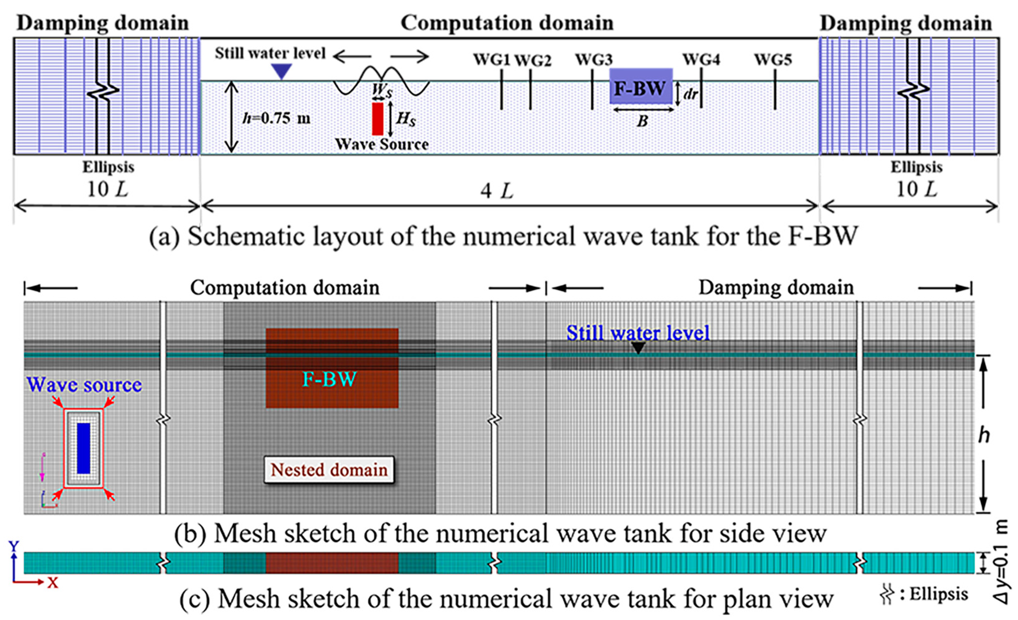
3.1. Numerical Wave Tank Setup

The detailed numerical wave tank (NWT) setup is shown in Figure 3b,c. The total length of the NWT was twenty-four wavelengths L long in the x-axis direction, 0.1 m wide in the y-axis direction, and 1 m deep in the z-axis direction. A scale ratio of 1:40 and a constant water depth h of 0.75 m are adopted based on the Froude similarity law. The mesh consisted of two distinct regions. The first region was the computation domain, four wavelengths length, with a width of 0.1 m and a depth of 1 m. The unit grid size of the total NWT was L/100~L/200 in the x and z directions, and ten grids were partitioned in the y directions in this domain. The second region was two identical damping domains with ten wavelength lengths. The Sommerfeld radiation method was employed to bate the secondary reflection of waves at both ends of the NWT. The grid size along the x-axis direction was gradually extended with an identical ratio of 1.01, and one grid was set for the lateral width of the NWT [38].
To describe the F-BW more accurately, nested grids were applied in the domain around the F-BW. The uniform nested grid was equal to half of the compute domain grid in the x, y and z-axis directions. Furthermore, the finer mesh resolution of 0.0035 cm in z direction was nested near the still water level (SWL), The region extends ±0.07 m from the SWL to ensure that the expected wave heights (0.03 m, 0.05 m, 0.07 m, 0.09 m) are encompassed within the region.
The boundary conditions of this NWT were set as follows: both ends of the NWT were defined as outflow boundaries, two sides of the domain were defined as symmetry boundaries, the atmospheric pressure was utilized at the upper boundary, and the lower surface of the computational domain was a no-slip wall boundary without surface roughness.
A mass source model with wide WS and high HS was added to the numerical flume. The symmetry boundaries were used overspreading with the mass source form, and the y-direction width of the mass source block was consistent with the width of the NWT. Pledging each edge of the mass block to coincide with the grid line of the NWT is shown in Figure 3b,c.

3.2. Numerical Model Validation

The present research is mainly implemented under the framework of CFD technology. To demonstrate the accuracy of the simulation results, it is essential to compare them with the extant results. The model is verified by the following three aspects in this section.

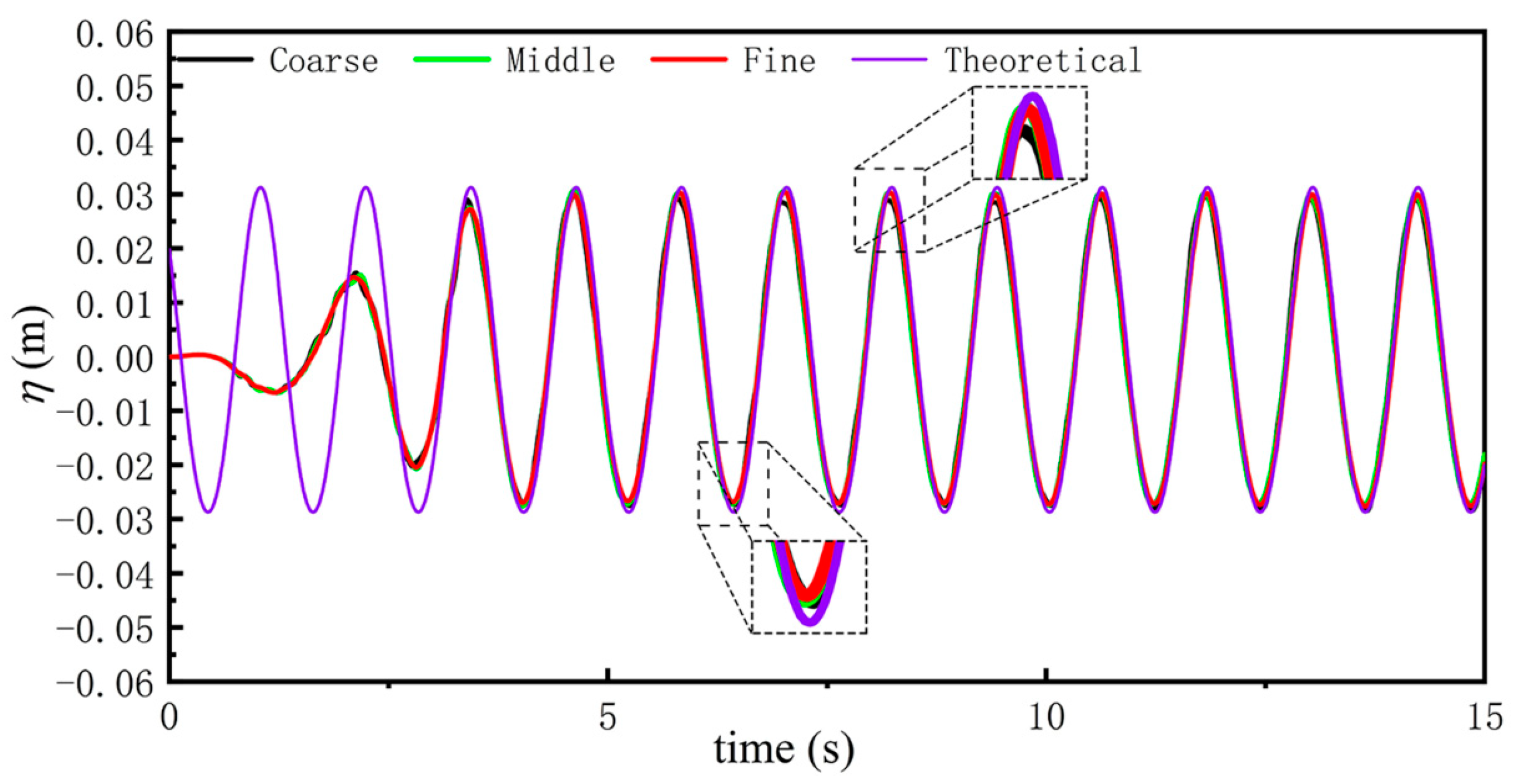
3.2.1. Grid Independent Verification

The mesh partition is a crucial procedure in CFD numerical simulation and needs much attention. The number and size of grids are essential criteria for evaluating the convergence of numerical results. Poor grid quality will directly affect the accuracy of numerical results and computation time. Consider that the proposed calculation cases Hi = 0.06 m, T = 1.2 s, and h = 1.2 m by Ren et al. are close to the target cases in this paper [23]. This wave condition is applied to complete the grid independence verification. Different grid arrangements can be seen in Table 2, and the time series of the wave profiles under the three grid sizes are compared with the theoretical results by solving Equation (5), as shown in Figure 5. The error of the numerical simulation results was calculated according to Equation (10). The wave profile deviations among the coarse mesh, medium mesh, and fine mesh are compared. The wave profiles under the medium mesh and the fine mesh are closer, and the deviation from the theoretical value is less than 5%, which meets the requirements of Det Norske Veritas (DNV) [39]. It can be judged that only medium meshes and refined meshes meet the requirements of numerical simulation. Considering the balance between calculation accuracy and calculation efficiency, the following numerical simulations always chose a medium mesh.
e r r o r = H t h e o r e t i c a l H n u m e r i c a l H t h e o r e t i c a l
where Htheoretical is the wave height of the theoretical result and Hnumerical is the wave height of the numerical result.

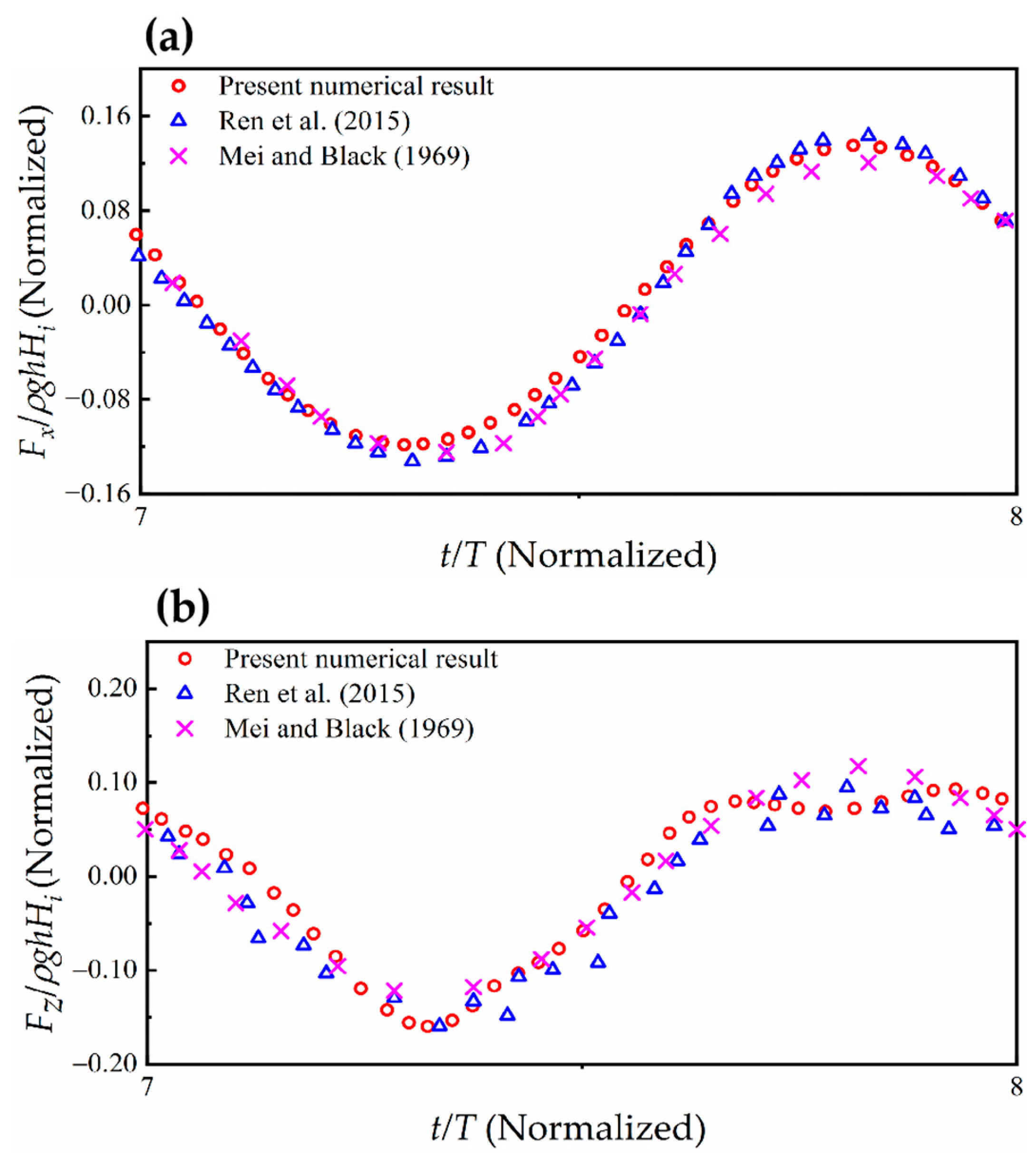
3.2.2. Validation of Wave Forces

In this section, to further inspect the accuracy of the numerical results of wave forces in this paper, according to the wave conditions of Hi = 0.06 m, T = 1.2 s, h = 1.2 m, and draft dr = 0.2 m, a rectangular box of width B = 0.8 m and wave height Hi = 0.4 m is fixed and semi-immersed, as proposed by Ren et al. [23]. The horizontal and vertical wave forces of the F-BW were verified by comparison with the theoretical results of Mei and Black [40] and the numerical simulation results of Ren et al. [23]. The time series of the wave forces are compared in Figure 6. The total simulation time of this case is 16 wave cycles. Since it takes some time for the progressive wave to arrive at the F-BW from the source, the horizontal and vertical wave forces begin to reach the stable state at t = 7 T seconds in Figure 6. By comparison, the simulated time series of horizontal and vertical wave forces are almost consistent with those presented by Ren et al. [23] and Mei and Black [40]. This result indicated that the present NWT could meet the calculation accuracy.

4. Results and Discussion

4.1. Influence Analysis of Four Factors on the Hydrodynamic Performance of F-BW

Among all the influencing factors (refer to Appendix A), the hydrodynamic performance of the F-BW is significantly affected by the following four factors: draft (dr/h), breakwater width (B/h), wave period (T*sqrt(g/h)), and wave height (Hi/h). For the mechanism analysis of the interaction between waves and breakwater, the mechanism study of the horizontal wave force is rather complicated. Since the breakwater is in a semisubmerged state, the Morison formula is no longer applicable to the guidance of the calculation of the horizontal wave force. The horizontal wave force is studied separately from the water particle velocity; see the free surface difference (η3–η4) in the front and back sides of the F-BW and the water particle streamline in Figure 7 and Figure 8 for details. Among them, five representative cases are selected from all cases in this article for comparative analysis corresponding to Figure 7a–e. Note that case (a) T1.2dr0.14B0.5Hi0.07 represents a wave period of 1.2 s, draft of 0.14 m, breakwater width of 0.5 m and incident wave height of 0.07 m. Due to the effect of water blockage, flow separation is generated at the bottom corner of the offshore side of the breakwater, and the generated clockwise vortex destroys the original motion path of the wave water particles without structure in Figure 8a and allows the free surface difference in the front and back of the F-BW to gradually reach a maximum. At time instant t0 in Figure 7, the horizontal wave force also reaches a maximum. It can be seen in Figure 8b that the vertical wave force is easier to analyze. When the vertical wave force is at its maximum, the streamline realizes complete diffraction, and no vortex is generated. Furthermore, to understand the mechanism and contribution of each influencing factor on the hydrodynamic performance of the F-BW in detail, the statistical results are shown in Figure 9, Figure 10, Figure 11 and Figure 12.

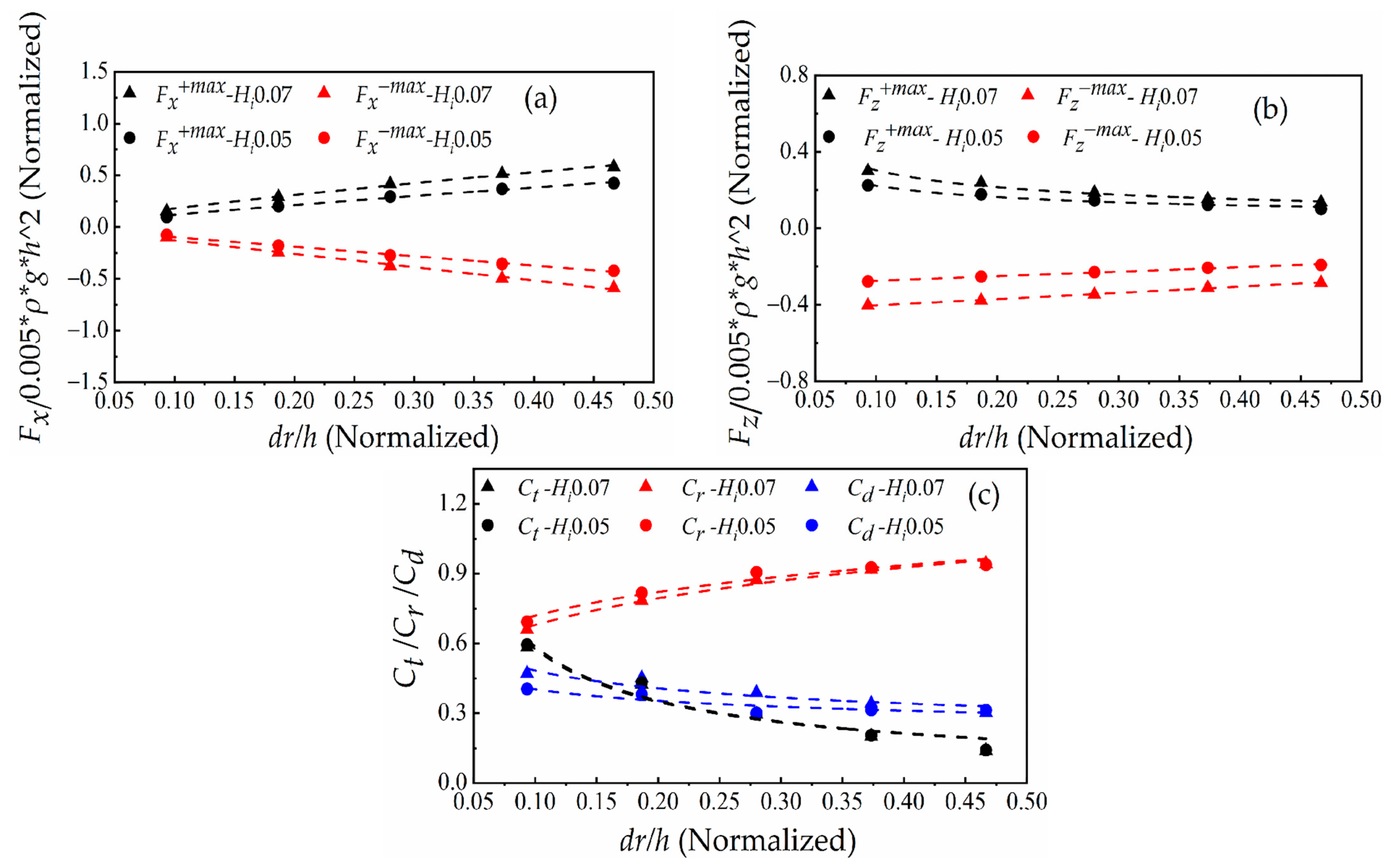
4.1.1. Effect of Draft

Figure 7 lists the distribution diagram of the free surface difference and water particle velocity under cases (a) and (b) at the time instant of the horizontal wave force maximum. Except for the draft being different, the two cases are consistent. Among them, case (a) has a wave period of 1.2 s, draft of 0.14 m, wave height of 0.07 m and breakwater width of 0.5 m. Case (b) has a period of 1.2 s, draft of 0.35 m, wave height of 0.07 m and breakwater width of 0.5 m.
In the second column of Figure 7a, when time t0 = 11.48 s, the maximum free surface difference is 0.068 m, and the maximum horizontal wave force is 7.98 N. In the second column of Figure 7b, when time t0 = 11.52 s, the maximum free surface difference is 0.083 m, and the maximum horizontal wave force is 15.91 N. Obviously, the increase in the draft enhances the water blockage action in front of the F-BW, weakens the diffraction effect of the wave, and delays the time for the horizontal wave force to reach its maximum. Figure 9a shows that Fx+max increases with increasing draft under wave heights of Hi = 0.05 m and Hi = 0.07 m. Similarly, the absolute values of Fxmax exhibit a similar law. The absolute values of Fzmax and Fz+max decrease with increasing draft under wave heights of Hi = 0.05 m and Hi = 0.07 m in Figure 9b, which is related to the exponential decay of the wave kinetic energy along the water depth. It is not difficult to see in Figure 7a,b that the wave hydrodynamic pressure on the lower surface of the F-BW decreases with decreasing wave kinetic energy as the water depth increases. The effective action area increases as the draft reduces the penetration of waves. Figure 9c shows that the transmission coefficient decreases with increasing draft under wave heights of Hi = 0.05 m and Hi = 0.07 m. Due to the increase in the interaction area between waves and F-BW, the reflected wave energy increases in Figure 7, and Figure 7b is more obvious than Figure 7a. The wave energy dissipation coefficient increases with decreasing draft in Figure 9c. Since the wave energy is mainly concentrated on the still water level, the fluid particle velocity maximum at the lower corner of F-BW is 0.30 m/s in Figure 7a is more than the 0.17 m/s in Figure 7b, more wave energy is dissipated when the fluid particle with higher velocity collides with F-BW due to decreasing draft.
Overall, the increasing draft impedes incident waves cross F-BW and promotes the increase in horizontal wave force and wave reflection, which threatens the stability of the structure.

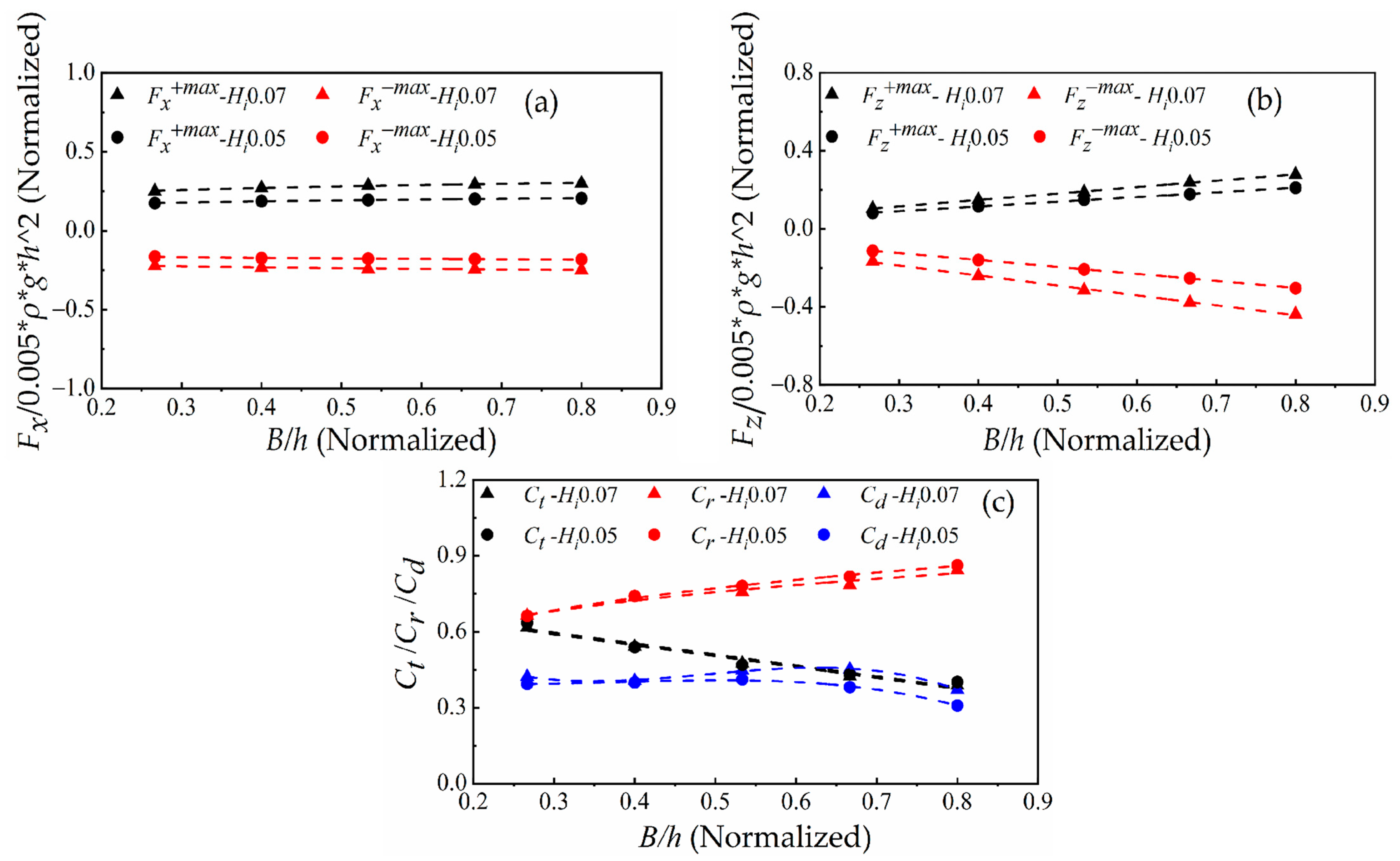
4.1.2. Effect of Breakwater Width

To clarify the mechanism of the breakwater width effect on the hydrodynamic performance of the F-BW, except that the breakwater width is different, cases (a) and (c) in Figure 7 are consistent. In case (c), the period is 1.2 s, the draft is 014 m, the wave height is 0.07 m, and the breakwater width is 0.2 m.
The free surface difference and vortex in Figure 7a,c are similar. Figure 10a shows that the breakwater width effect on Fxmax and Fx+max is not obvious. When the vertical wave force is at its maximum, the streamline realizes complete diffraction, and no vortex is generated in Figure 8b. Therefore, the vertical wave force is related to the acting area of the F-BW lower surface. Figure 10b shows that the absolute values of Fzmax and Fz+max increase with increasing breakwater width. In the second column of Figure 7c, when time t0 = 11.42 s, the free surface difference and the horizontal wave force reach a maximum faster than in case (a). Obviously, the increase in the breakwater width increases the wave diffraction difficulty. Figure 10c shows that the transmission coefficient decreases with increasing breakwater width, and the reflection coefficient increases with increasing breakwater width. Due to fluid particle velocity maximum is similar between Figure 7a,c. The increase in breakwater width has little influence on wave energy dissipation.
In short, the increasing breakwater width is not conducive to incident wave cross F-BW, and promotes the increase of wave reflection and vertical wave force. Obviously, more weights need to be added to ensure the safety of the breakwater when breakwater width increases.

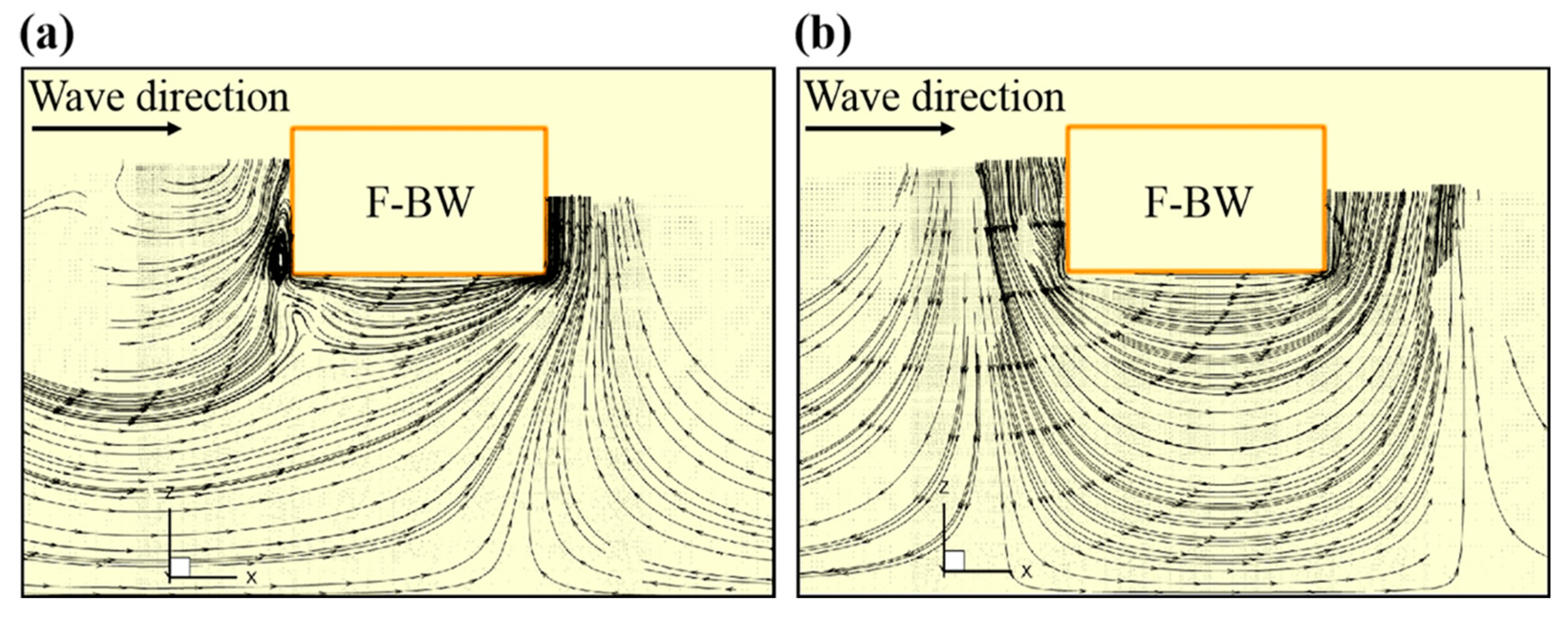
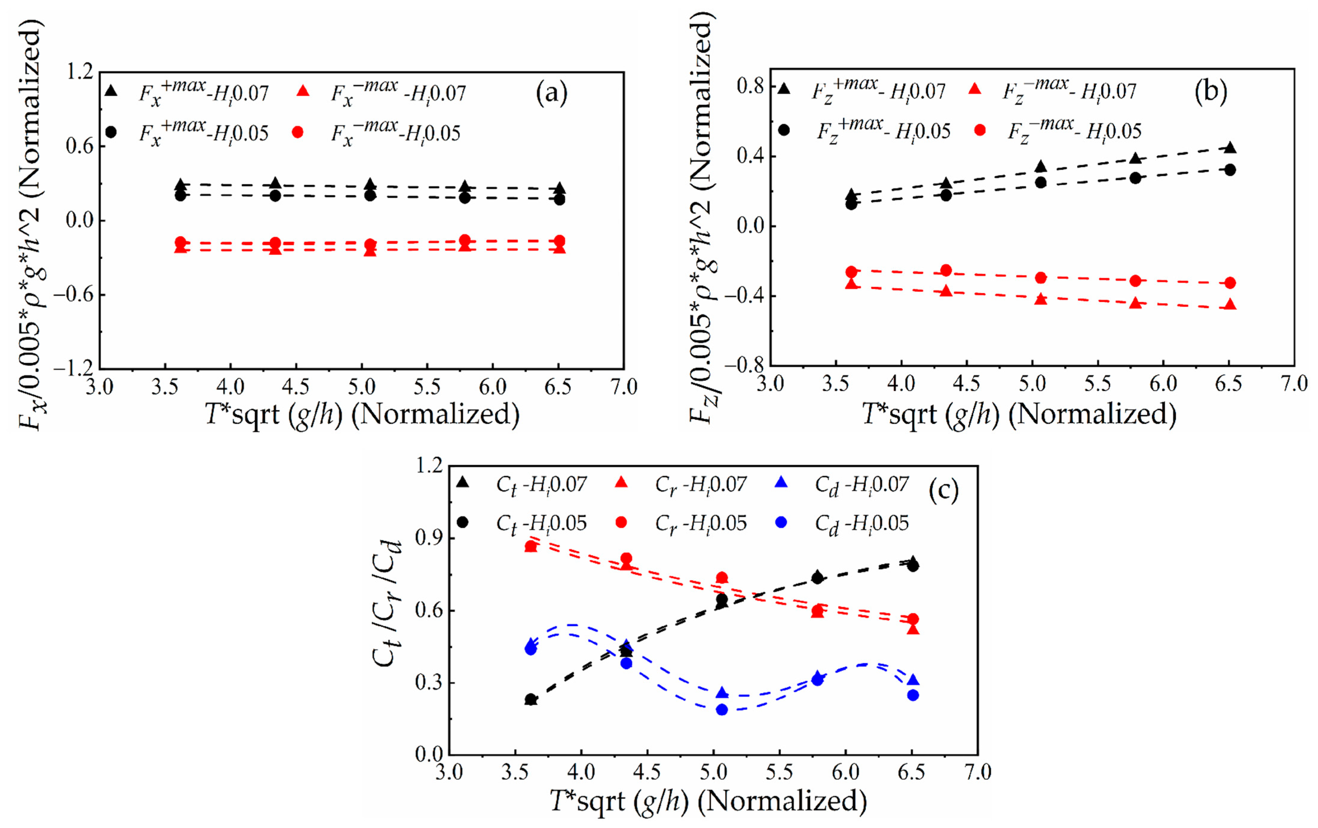
4.1.3. Effect of Wave Period

To clarify the mechanism of the wave period effects on the hydrodynamic performance of the breakwater, except that the wave period is different, cases (a) and (d) are consistent. Figure 7d shows that the wave period is 1.8 s, the draft is 0.14 m, the wave height is 0.07 m and the breakwater width is 0.5 m.
In the second column of Figure 7d, when time t0 = 11.13 s, the maximum free surface difference is 0.051 m, and the maximum horizontal wave force is 6.90 N. According to Equation (9), because the wave energy is more abundant on the two sides of the breakwater in case (4), the horizontal wave force is comparable even if the free surface difference is smaller than that in case (1). Figure 11a shows that Fxmax and Fx+max are weakly related to the wave period under wave heights of Hi = 0.05 m and Hi = 0.07 m. Because the long-period waves possess a large wave energy in Figure 7d, they increase the wave pressure on the lower surface of the F-BW. Therefore, the absolute values of Fzmax and Fz+max increase linearly with the wave period in Figure 11b. Figure 11c shows that the transmission coefficient increases with increasing wave period under wave heights of Hi = 0.05 m and Hi = 0.07 m. Long-period waves have a better diffraction ability at the same depth, and more wave energy passes through the F-BW. The decreasing ratio of the breakwater width to wavelength weakens the ability to block progressive waves, and the reflection coefficient decreases accordingly. The wave energy dissipation coefficient shows an alphabetic symbol “M” distribution with the wave period. This indicates that the wave energy dissipation is more complex and requires further study. When the dimensionless wave period is 5.06, both the transmission and reflection coefficients are close to 0.71, the dissipation coefficient is at the minimum by applying Equation (8c).
In brief, the increasing wave period plays a significant role in increasing the wave transmission and the reducing wave reflection. Although it has little effect on the horizontal wave force, it promotes an increase in the vertical wave force, which is unfavorable to the security of the breakwater.

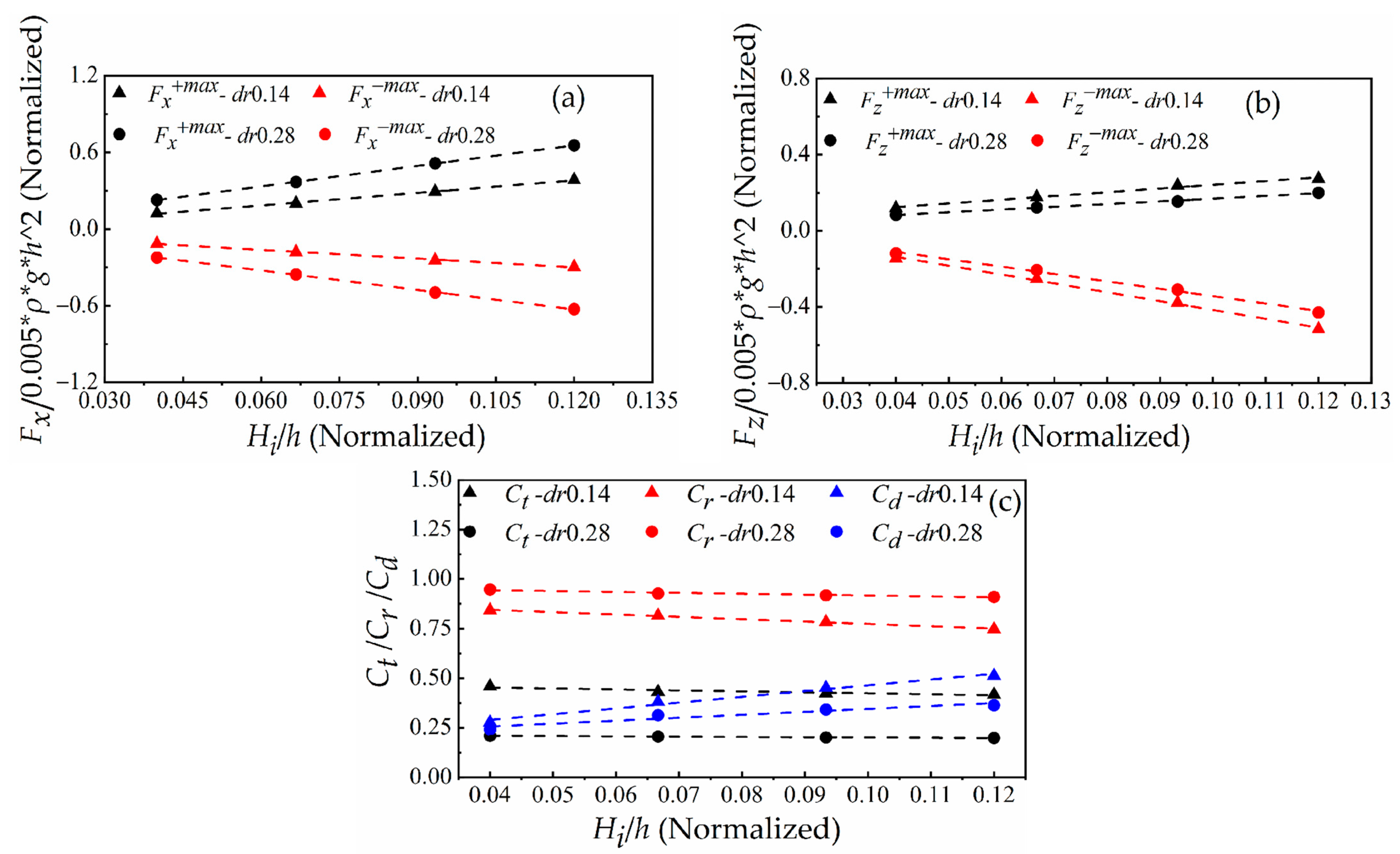
4.1.4. Effect of Wave Height

To clarify the mechanism of the wave height effects on the hydrodynamic performance of the breakwater, except that the wave height is different, cases (a) and (e) are consistent. Figure 7e shows that the wave period is 1.2 s, the draft is 014 m, the wave height is 0.03 m and the breakwater width is 0.5 m.
In the second column of Figure 7e, when time t0 = 11.44 s, the maximum free surface difference is 0.031 m, and the maximum horizontal wave force is 3.43 N. Obviously, the increase in wave height increases the diffraction difficulty of the wave and delays the time when the horizontal wave force reaches its maximum. The higher the wave height, the more abundant the wave energy in Figure 7a,e. The water particle velocity maximum is 0.11 m/s in Figure 7e, which is much less than the water particle velocity maximum in Figure 7a. The larger wave height causes a larger wave elevation difference, and the larger horizontal wave force under other variable conditions is consistent by comparing Figure 7a,e. Therefore, Fxmax and Fx+max increase linearly with increasing wave height under drafts dr = 0.14 m and dr = 0.28 m in Figure 12a. The increase in wave height leads to increasing dynamic wave pressure, which in turn leads to increasing wave pressure on the F-BW lower surface and an increase in vertical wave force. Therefore, Fzmax and Fz+max increase linearly with increasing wave height under drafts dr = 0.14 m and dr = 0.28 m in Figure 12b. Figure 12c shows that the increasing wave height results in more wave reflection and less transmission due to the increasing blockage effect. The reflection ability weakens with decreasing interaction area (the ratio of the wetted surface height of the front wall of the F-BW to the wave height). The water particle velocity maximum of 0.11 m/s in Figure 7e is less than the water particle velocity maximum of 0.3 m/s in Figure 7a. The increasing water particle velocity with increasing wave height results in better vortex dissipation near the F-BW. Hence, the wave energy dissipation coefficient increases.
In conclusion, the increasing wave height reduces the wave reflection but increases horizontal and vertical wave forces, which is disadvantageous to the security of the breakwater.

4.2. Prediction Equations of F-BW Hydrodynamic Performance Parameters

To understand the contribution of each influencing factor to the hydrodynamic performance of the F-BW in detail, the factors affecting the RTD coefficients and wave force mainly include the wave period T, wave height Hi, draft dr, breakwater width B, and still water depth h. In Equation (11), the RTD coefficients Ct,r,d and wave force extremum Fx,z±max are expressed as follows:
( F x , z ± m a x , C t , r , d ) = f h , T , ρ , H i , d r , B , g
Using the dimensionless analysis method and the numerical simulation results of 30 groups of simulated conditions in Table 1 based on the Origin 2019b software platform, multiple linear regression was performed by the least squares method, and the prediction equations of the RTD coefficients and wave force are given in Equation (12a–g). The detailed formulas are shown in Table 3.
Note that 0.0933 ≤ dr/h ≤ 0.4667, 0.26667 ≤ B/h ≤ 0.8, 3.6166 ≤ T*sqrt(g/h) ≤ 6.5099, and 0.04 ≤ Hi/h ≤ 0.12.

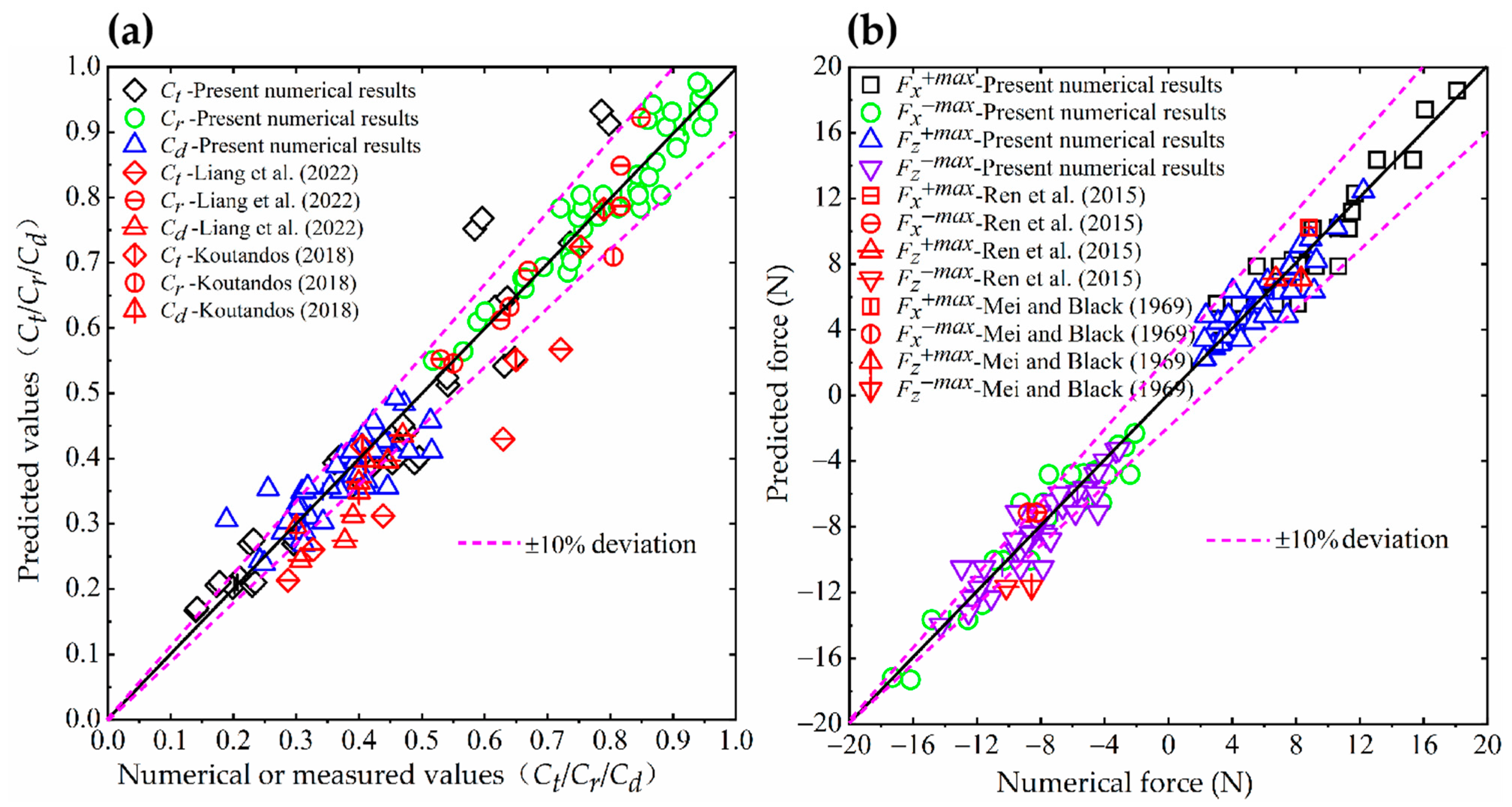
4.3. Deviation Analysis of the Prediction Equations

Inspired by Kurdistani et al.’s [24] research method, the current study uses their method to assess the reliability of each predictive formula. The literature observation datasets include the measured RTD coefficients from Koutandos [13] (three cases (R1, R2 and R3) in Figure 16 of his literature) and Liang et al. [14] (six cases in Figures 14a, 19a and 22a of their literature), the wave forces from Mei and Black [40] and Ren et al. [23] (a case in Figure 10 of their literature). The numerical results obtained by Flow-3D are plotted on the x-axis in Figure 13, and predicted values of the predictive equations are plotted on the y-axis in Figure 13. Figure 13a shows a 20% error for the application of Liang et al. [14] transmission coefficient datasets that are mostly lower-estimated values of transmission coefficient with respect to Equation (12a), an almost 10% error for the application of Liang et al.’s [14] reflection coefficient and dissipation coefficient datasets, and Koutandos’s [13] RTD coefficients datasets. Figure 13b shows an almost 10% error for the application of Mei and Black [40] and Ren et al. [23] maximum wave force, which indicates that the present prediction equations are valid.
It is clearly found that the distribution points of the reflection coefficient and wave energy dissipation coefficient of the F-BW are relatively concentrated in a particular region in Figure 13a, indicating that the F-BW is dominant in reflecting waves and has stable wave dissipation ability. In addition, the horizontal negative maximum wave force of the F-BW is similar to the vertical negative maximum wave force, and the horizontal positive maximum wave force of the F-BW is slightly larger than the vertical positive maximum wave force in Figure 13b.

5. Conclusions

The present study investigated a high-accuracy numerical wave tank (NWT) based on the Flow-3D platform. A series of numerical simulations in the intermediate waters were carried out at a constant water depth (h) of 0.75 m under regular wave conditions, with a wave height range between 0.03–0.09 m, a wave period range between 1–1.8 s, and a breakwater width range between 0.2–0.6 m. The effects of four influencing factors (dr, B, T, Hi) on the hydrodynamic performance (RTD coefficients and wave forces) are highlighted. The vital conclusions are as follows:
(1)
The performance of two-dimensional viscous numerical wave tanks (NWTs) with a mass source wave maker and small length scale (1:40) are analyzed. By comparison, the wave model employed in this paper is competent for the numerical simulation of the F-BW.
(2)
The results show that the increase in the four influence factors, except the wave period, benefits the decrease in the wave transmission. The increase in draft and breakwater width is beneficial to the increase in the wave reflection, and the wave period and wave height are opposite. The increase in draft benefits the decrease in wave energy dissipation, and the wave height is opposite.
(3)
The increase in the draft and wave height benefits the increase in the horizontal positive and negative maximum wave forces. In addition to the draft, the increase in the other three influence factors benefits the increase in the vertical positive and negative maximum wave forces.
(4)
Applying multiple linear regression presents the prediction equations of RTD coefficients and the extreme wave force. The prediction equations are verified by comparing them with literature observation datasets.
This study provides insight into the relation of RTD coefficients and wave forces with parameters such as draft, breakwater width, wave period and wave height. The simulated results of the given predicted equations can be generalized to the prototype scale by using Froude’s scaling law and can be used to guide the design of F-BWs in intermediate waters.

Author Contributions

Conceptualization and methodology, G.N., N.F. and Y.C.; software, J.L. and G.N.; visualization, J.Z. and N.F.; writing—original draft, G.N. and N.F.; writing—review and editing, G.N., N.F. and J.L.; supervision, N.F. and Y.C. All authors have read and agreed to the published version of the manuscript.

Funding

The work presented here was supported by the Science and Technology Innovation Serve Project of Wenzhou Association for Science and Technology (No. kjfw65), the General Scientific Research Project of Education Department of Zhejiang Province (Y202250703), the National Natural Science Foundation of China (52108337), the Basic Scientific Research Project of Wenzhou City (No. S20220033), the Wenzhou Science and Technology Commissioners Project (X20210087), and the Wenzhou Basic Public Scientific Research Project (2023S0109).

Institutional Review Board Statement

Not applicable.

Informed Consent Statement

Not applicable.

Data Availability Statement

The original contributions presented in the study are included in the article. Further inquiries can be directed to the corresponding author.

Acknowledgments

The assistance of Yongchun Yang and Baochang Zhang, of the Ocean University of China’s College of Engineering, received during the course of the numerical experiments, is greatly appreciated.

Conflicts of Interest

The authors declare that the research was conducted in the absence of any commercial or financial relationships that could be construed as a potential conflict of interest.

Appendix A

The wave period T, wave height Hi, draft dr, breakwater width B, and water depth h are the main factors that affect the wave dissipation performance and wave force of an F-BW in the intermediate waters. Therefore, the wave force of an F-BW can be expressed as a function of the above factors as follows:
F = f h , T , ρ , H i , d r , B , g
Taking water depth h, gravity acceleration g, and water density ρ as the repetitive parameters, the three dimensionless parameters are expressed as follows:
[h] = [M0L1T0], [g] = [M0L1T−2], [ρ] = [M1L−3T0], where wave force per breakwater length in the vertical wave direction F , expressed as [F = ρgh2], Equation (A1) can be written as follows:
F 0.005 ρ g h 2 = f ( d r h , B h , T g h , H i h )
According to wave theory, there is a nonlinear relationship between the wave force and the four dimensionless parameters in Equation (A2). The relationship between the dependent variable and independent variable in nature is exponential. It can be expressed as follows:
F 0.005 ρ g h 2 = α d r h x 1 B h x 2 T g h x 3 H i h x 4
where α, x1, x2, x3, and x4 are the unknown coefficients.
Taking the natural logarithm of both sides of Equation (A3) to obtain the double logarithm function model, the equation can be written in linear form as follows:
ln F 0.005 ρ g h 2 = ln α + x 1 ln d r h + x 2 ln B h + x 3 ln T g h + x 4 ln H i h
Using multiple function linear regression analysis, each unknown coefficient in the equations can be obtained and then substituted into Equation (A3) to obtain the wave force equations. Similarly,
C t , C r , C d = f d r h , B h , T g h , H i h

References

  1. He, F.; Huang, Z.H.; Law, A.W.K. Hydrodynamic performance of a rectangular floating breakwater with and without pneumatic chambers: An experimental study. Ocean Eng. 2012, 51, 16–27. [Google Scholar] [CrossRef]
  2. Zhan, J.; Chen, X.; Gong, Y.; Hu, W. Numerical investigation of the interaction between an inverse T-type fixed/floating breakwater and regular/irregular waves. Ocean Eng. 2017, 137, 110–119. [Google Scholar] [CrossRef]
  3. Fu, D.; Zhao, X.Z.; Wang, S.; Yan, D.M. Numerical study on the wave dissipating performance of a submerged heaving plate breakwater. Ocean Eng. 2021, 219, 108310. [Google Scholar] [CrossRef]
  4. Hales, L.Z. Floating Breakwaters: State-of-the-Art Literature Review; Coastal Engineering Research Center: London, UK, 1981. [Google Scholar]
  5. Teh, H.M. Hydraulic performance of free surface breakwaters: A review. Sains Malays. 2013, 42, 1301–1310. [Google Scholar]
  6. Liang, J.M.; Chen, Y.K.; Liu, Y.; Li, A.J. Hydrodynamic performance of a new box-type breakwater with superstructure: Experimental study and SPH simulation. Ocean Eng. 2022, 266, 112819. [Google Scholar] [CrossRef]
  7. Zhao, X.L.; Ning, D.Z. Experimental investigation of breakwater-type WEC composed of both stationary and floating pontoons. Energy 2018, 155, 226–233. [Google Scholar] [CrossRef]
  8. Macagno, A. Wave action in a flume containing a submerged culvert. In La Houille Blanche; Taylor and Francis: London, UK, 1954. [Google Scholar]
  9. Wiegel, R.L. Transmission of waves past a rigid vertical thin barrier. J. Waterw. Harb. Div. 1960, 86, 1–12. [Google Scholar] [CrossRef]
  10. Ursell, F. The effect of a fixed vertical barrier on surface waves in deep water. Math. Proc. Camb. Philos. Soc. 1947, 43, 374–382. [Google Scholar] [CrossRef]
  11. Guo, Y.; Mohapatra, S.C.; Guedes Soares, C. Wave interaction with a rectangular long floating structure over flat bottom. In Progress in Maritime Technology and Engineering; CRC Press: Boca Raton, FL, USA, 2018; pp. 647–654. [Google Scholar]
  12. Kolahdoozan, M.; Bali, M.; Rezaee, M.; Moeini, M.H. Wave-transmission prediction of π-type floating breakwaters in intermediate waters. J. Coast. Res. 2017, 33, 1460–1466. [Google Scholar] [CrossRef]
  13. Koutandos, E. Regular-irregular wave pressures on a semi-immersed breakwater. J. Mar. Environ. Eng. 2018, 10, 109–145. [Google Scholar]
  14. Liang, J.M.; Liu, Y.; Chen, Y.K.; Li, A.J. Experimental study on hydrodynamic characteristics of the box-type floating breakwater with different mooring configurations. Ocean Eng. 2022, 254, 111296. [Google Scholar] [CrossRef]
  15. Fugazza, M.; Natale, L. Energy losses and floating breakwater response. J. Waterw. Port Coast. Ocean Eng. 1988, 114, 191–205. [Google Scholar] [CrossRef]
  16. Koftis, T.; Prinos, P. 2 DV Hydrodynamics of a Catamaran-Shaped Floating Structure. Iasme Trans. 2005, 2, 1180–1189. [Google Scholar]
  17. Elsharnouby, B.; Soliman, A.; Elnaggar, M.; Elshahat, M. Study of environment friendly porous suspended breakwater for the Egyptian Northwestern Coast. Ocean Eng. 2012, 48, 47–58. [Google Scholar] [CrossRef]
  18. Chen, Y.; Niu, G.; Ma, Y. Study on hydrodynamics of a new comb-type floating breakwater fixed on the water surface. In Proceedings of the E3S Web of Conferences, Wuhan, China, 14–16 December 2018; EDP Sciences: Les Ulis, France, 2018; Volume 79, p. 02003. [Google Scholar]
  19. Fan, N.; Nian, T.K.; Jiao, H.B.; Guo, X.S.; Zheng, D.F. Evaluation of the mass transfer flux at interfaces between submarine sliding soils and ambient water. Ocean Eng. 2020, 216, 108069. [Google Scholar] [CrossRef]
  20. Fan, N.; Jiang, J.X.; Dong, Y.K.; Guo, L.; Song, L.F. Approach for evaluating instantaneous impact forces during submarine slide-pipeline interaction considering the inertial action. Ocean Eng. 2022, 245, 110466. [Google Scholar] [CrossRef]
  21. Ghafari, A.; Tavakoli, M.R.; Nili-Ahmadabadi, M.; Teimouri, K.; Kim, K.C. Investigation of interaction between solitary wave and two submerged rectangular obstacles. Ocean Eng. 2021, 237, 109659. [Google Scholar] [CrossRef]
  22. Zheng, X.; Lv, X.P.; Ma, Q.W.; Duan, W.Y.; Khayyer, A.; Shao, S.D. An improved solid boundary treatment for wave–float interactions using ISPH method. Int. J. Nav. Archit. Ocean Eng. 2018, 10, 329–347. [Google Scholar] [CrossRef]
  23. Ren, B.; He, M.; Dong, P.; Wen, H.J. Nonlinear simulations of wave-induced motions of a freely floating body using WCSPH method. Appl. Ocean Res. 2015, 50, 1–12. [Google Scholar] [CrossRef]
  24. Kurdistani, S.M.; Tomasicchio, G.R.; D’Alessandro, F.; Francone, A. Formula for Wave Transmission at Submerged Homogeneous Porous Breakwaters. Ocean Eng. 2022, 266, 113053. [Google Scholar] [CrossRef]
  25. Hirt, C.W.; Nichols, B.D. Flow-3D User’s Manuals; Flow science Inc.: Santa Fe, NM, USA, 2012. [Google Scholar]
  26. Yakhot, V.; Orszag, S.A. Renormalization group analysis of turbulence. I. Basic theory. J. Sci. Comput. 1986, 1, 3–51. [Google Scholar] [CrossRef]
  27. Hirt, C.W.; Nichols, B.D. Volume of fluid (VOF) method for the dynamics of free boundaries. J. Comput. Phys. 1981, 39, 201–225. [Google Scholar] [CrossRef]
  28. Saad, Y.; Schultz, M.H. GMRES: A generalized minimal residual algorithm for solving nonsymmetric linear systems. SIAM J. Sci. Stat. Comput. 1986, 7, 856–869. [Google Scholar] [CrossRef]
  29. Faraci, C.; Musumeci, R.E.; Marino, M.; Ruggeri, A.; Carlo, L.; Jensen, B.; Foti, E.; Barbaro, G.; Elsaßer, B. Wave-and current-dominated combined orthogonal flows over fixed rough beds. Cont. Shelf Res. 2021, 220, 104403. [Google Scholar] [CrossRef]
  30. Lin, P.Z.; Liu, P.L.-F. Internal wave-maker for Navier-Stokes equations models. J. Waterw. Port Coast. Ocean Eng. 1999, 125, 207–215. [Google Scholar] [CrossRef]
  31. Lara, J.L.; Garcia, N.; Losada, I.J. RANS modelling applied to random wave interaction with submerged permeable structures. Coast. Eng. 2006, 53, 395–417. [Google Scholar] [CrossRef]
  32. Ha, T.; Lin, P.Z.; Cho, Y.S. Generation of 3D regular and irregular waves using Navier-Stokes equations model with an internal wave maker. Coast. Eng. 2013, 76, 55–67. [Google Scholar] [CrossRef]
  33. Chen, Y.L.; Hsiao, S.C. Generation of 3D water waves using mass source wavemaker applied to Navier-Stokes model. Coast. Eng. 2016, 109, 76–95. [Google Scholar] [CrossRef]
  34. Windt, C.; Davidson, J.; Schmitt, P.; Ringwood, J.V. On the assessment of numericalwave makers in CFD simulations. J. Mar. Sci. Eng. 2019, 7, 47. [Google Scholar] [CrossRef]
  35. Wang, D.X.; Dong, S. Generating shallow-and intermediate-water waves using a line-shaped mass source wavemaker. Ocean Eng. 2021, 220, 108493. [Google Scholar] [CrossRef]
  36. Wang, D.X.; Sun, D.; Dong, S. Numerical investigation into effect of the rubble mound inside perforated caisson breakwaters under random sea states. Proc. Inst. Mech. Eng. Part M J. Eng. Marit. Environ. 2022, 236, 48–61. [Google Scholar] [CrossRef]
  37. Goda, Y.; Suzuki, Y. Estimation of incident and reflected waves in random wave experiments. In Proceedings of the 15th International Conference on Coastal Engineering, Honolulu, HI, USA, 11–17 July 1976; pp. 828–845. [Google Scholar]
  38. Orlanski, I. A simple boundary condition for unbounded hyperbolic flows. J. Comput. Phys. 1976, 21, 251–269. [Google Scholar] [CrossRef]
  39. Veritas, D.N. Environmental Conditions and Environmental Loads: Recommended Practice; DNV-RP-C205; Det Norske Veritas (DNV): Oslo, Norway, 2010. [Google Scholar]
  40. Mei, C.C.; Black, J.L. Scattering of surface waves by rectangular obstacles in waters of finite depth. J. Fluid Mech. 1969, 38, 499–511. [Google Scholar] [CrossRef]
Figure 1. Two-dimensional schematic sketch of the F-BW models.
Jmse 11 01812 g001
Figure 2. Wave parameter conditions analyzed in this study and their relations in the Le Méhauté diagram.
Jmse 11 01812 g002
Figure 3. Schematic layout and mesh sketch of the numerical wave tank for the F-BW.
Jmse 11 01812 g003
Figure 4. Time histories of wave elevation η measured by WG1, WG2, and WG5 and horizontal and vertical wave forces of F-BW at Hi = 0.07 m, T = 1.4 s, B = 0.5 m, dr = 0.14 m, and h = 0.75 m.
Jmse 11 01812 g004
Figure 5. Grid independent verification: influence of mesh size on wave profile.
Jmse 11 01812 g005
Figure 6. Comparison of the normalized wave force on an F-BW with previous studies (Mei and Black [40]; Ren et al. [23]). (a) Normalized horizontal wave force; (b) Normalized vertical wave force.
Jmse 11 01812 g006
Figure 7. Comparative analysis of five different cases under the interaction between waves and breakwater: First column: numerically obtained snapshots of free surface profile and velocity field; Second column: time history of free surface and horizontal wave force.
Jmse 11 01812 g007
Figure 8. Snapshots of the velocity streamline field: (a) Time instant of the horizontal positive maximum wave force; (b) Time instant of the vertical positive maximum wave force.
Jmse 11 01812 g008
Figure 9. Effect of the draft dr on the hydrodynamic performance of the F-BW at wave heights Hi = 0.05 m and Hi = 0.07 m. (a) Horizontal positive and negative maximum wave forces Fx+max and Fxmax; (b) Vertical positive and negative maximum wave forces Fz+max and Fzmax; (c) Transmission coefficient Ct, reflection coefficient Cr, and dissipation coefficient Cd.
Jmse 11 01812 g009
Figure 10. Influence of the breakwater width B on the hydrodynamic performance of the F-BW at wave heights Hi = 0.05 m and Hi = 0.07 m. (a) Horizontal positive and negative maximum wave forces Fx+max and Fxmax; (b) Vertical positive and negative maximum wave forces Fz+max and Fzmax; (c) Transmission coefficient Ct, reflection coefficient Cr, and dissipation coefficient Cd.
Jmse 11 01812 g010
Figure 11. Influence of the wave period T on the hydrodynamic performance of the F-BW at wave heights Hi = 0.05 m and Hi = 0.07 m. (a) Horizontal positive and negative maximum wave forces Fx+max and Fxmax; (b) Vertical positive and negative maximum wave forces Fz+max and Fzmax; (c) Transmission coefficient Ct, reflection coefficient Cr, and dissipation coefficient Cd.
Jmse 11 01812 g011
Figure 12. Influence of the wave height Hi on the hydrodynamic performance of the F-BW at draft dr = 0.14 m and dr = 0.28 m. (a) Horizontal positive and negative maximum wave forces Fx+max and Fxmax; (b) Vertical positive and negative maximum wave forces Fz+max and Fzmax; (c) Transmission coefficient Ct, reflection coefficient Cr, and dissipation coefficient Cd.
Jmse 11 01812 g012
Figure 13. Comparison of the results between previous studies and the numerical results of this study. (a) Transmission coefficient Ct, reflection coefficient Cr, and dissipation coefficient Cd (Koutandos [13], Liang et al. [14]) and (b) Maximum wave force (Mei and Black [40]; Ren et al. [23]).
Jmse 11 01812 g013
Table 1. Summary of the simulated scenarios.
Variable 1Variable 2Variable 3Variable 4
drBTHi
[m][m][s][m]
Case 10.070.051.20.05
Case 20.07
Case 30.140.05
Case 40.07
Case 50.210.05
Case 60.07
Case 70.280.05
Case 80.07
Case 90.350.05
Case 100.07
Case 110.140.21.20.05
Case 120.07
Case 130.30.05
Case 140.07
Case 150.40.05
Case 160.07
Case 170.60.05
Case 180.07
Case 190.140.510.05
Case 200.07
Case 211.40.05
Case 220.07
Case 231.60.05
Case 240.07
Case 251.80.05
Case 260.07
Case 270.140.51.20.03
Case 280.28
Case 290.140.09
Case 300.28
Table 2. Mesh independence check results.
Mesh TypeComputation Domain Grid Size (cm)Nested Domain Grid Size (cm)Cell NumberElapsed Time (×104 s)Wave Height (cm)Error %
Coarse217014600.64965.6425.96
Middle10.534111807.68325.7683.87
Fine0.50.251335096048.14375.7693.85
Theoretical----6.000-
Table 3. Statistics of prediction equation.
Equation NumberEquationsR2
(12a) C t = 0.003 d r h 0.935 B h 0.519 g T 2 h 1.039 H i h 0.064 0.948
(12b) C r = 3.650 d r h 0.213 B h 0.187 g T 2 h 0.436 H i h 0.074 0.958
(12c) C d = 3.100 d r h 0.235 B h 0.113 g T 2 h 0.493 H i h 0.426 0.695
(12d) F x + m a x 0.005 ρ g h 2 = 21.398 d r h 0.866 B h 0.139 g T 2 h 0.127 H i h 1.027 0.992
(12e) F x m a x 0.005 ρ g h 2 = 14.199 d r h 1.062 B h 0.057 g T 2 h 0.042 H i h 0.912 0.988
(12f) F z + m a x 0.005 ρ g h 2 = 0.079 d r h 0.519 B h 0.852 g T 2 h 0.829 H i h 0.798 0.988
(12g) F z m a x 0.005 ρ g h 2 = 2.314 d r h 0.254 B h 0.890 g T 2 h 0.282 H i h 1.145 0.989
Disclaimer/Publisher’s Note: The statements, opinions and data contained in all publications are solely those of the individual author(s) and contributor(s) and not of MDPI and/or the editor(s). MDPI and/or the editor(s) disclaim responsibility for any injury to people or property resulting from any ideas, methods, instructions or products referred to in the content.

