Article

Phase-Resolved Wave Simulation over Isolated Seamount

by
Arnida L. Latifah
1,2,*,
Henokh Lugo Hariyanto
1,†,
Durra Handri
1 and
E. van Groesen
1
1
LabMath-Indonesia, Jl. Dago Giri No. 99, Bandung 40391, Indonesia
2
Research Center for Computing, National Research and Innovation Agency, Jl. Raya Jakarta-Bogor KM 47, Bogor 16911, Indonesia
*
Author to whom correspondence should be addressed.
Current address: Information System, Kalimantan Institute of Technology, Balikpapan 76127, Indonesia.
J. Mar. Sci. Eng. 2023, 11(9), 1765; https://doi.org/10.3390/jmse11091765
Submission received: 4 August 2023 / Revised: 6 September 2023 / Accepted: 7 September 2023 / Published: 9 September 2023

Abstract

:
This paper investigates the wind wave deformations above two isolated shallow seamounts using a phase-resolved wave model simulation using the HAWASSI-AB software. The first seamount is located some 8 km from the south coast of Jawa, Indonesia, near Glagah, with its top area about 2 m from the water level, while the second is the Socotra Rock, in the East China Sea, which has a top 4.6 m under the sea surface. The simulations found that isolated shallow bathymetry may generate a crossing sea region endangering ships. In both domains, short-crested wave simulations of second order show strong refraction and diffraction effects when waves run towards and downstream of the top of the seamount. Waves near the summit embrace the seamount and form a focal area with larger waves downstream. After crossing the Socotra Rock, the interaction waves lead to a crossing sea in the deep water. On the other hand, having passed the Glagah, waves further downstream are partly absent over a substantial stretch of the coast. For both cases, the phase-resolved wave simulation results determine detailed wind wave conditions and wave spectra over the whole area, compensating for a lack of experimental data.

1. Introduction

Coastal wave research, experiments, and simulations are important for protective measures, sedimentation studies, and the design of coastal structures such as harbors and dikes near the coast. Wave research in the open ocean is also essential for the safety of structures and navigation. Apart from measurements in the field or environmental laboratories, numerical simulations are commonly used to obtain more extensive information about the expected wave transformations and their interaction with structures, bathymetry, or the beach. Wave interactions with a complex bathymetry with a shallow part are interesting as the waves may behave abnormally, which can endanger ships and structures. The study by [1] showed that shallow bathymetry in the open ocean may also affect the global ocean. They revealed that nonlinear internal wave fronts radiating from a shallow sill bathymetry on a broad shelf have substantial implications for transporting and redistributing heat, energy, momentum, and materials in the global coastal ocean as well as the regional East China Sea.
Shallow seamounts can be found abundantly worldwide. A database of nearly 25,000 seamounts [2] gives extensive information about global seamounts, including their locations and approximate sizes. The water depth in which seamounts are found can vary from bottomless to very shallow water. Larger seamounts will disturb ocean circulation and, depending on their size and the water depth above the top, their presence may perturb the surface waves. Thus, shallow seamounts are a concern for navigation around shipping routes, as the wind-wave field surrounding them can be very peculiar [3].
Theoretical research on the effects of the presence of seamounts on the surrounding waves started with [4,5]; see also [6]. Early numerical simulations of the flow dynamics around a seamount used a large-scale ocean circulation model; see, e.g., [7,8,9]. Ocean simulations dealing with seamounts studied the effect of their presence on the surrounding oceanic flow, such as mixing and turbulence effects; see, for instance, [10,11,12]. Numerical wave simulations based on a phase-averaged wave model over smaller ocean domains were conducted by [3]. Their study modeled the Socotra Rock, which has a top just 4.6 m below the sea surface in the Yellow Sea. Meanwhile, [13] also used a phase-averaged wave model to compare numerical wave simulation results with observations over domains with top heights of 21, 42, and 54 m, near the coast of north Brazil.
Numerical simulations using a phase-averaged wave model are able to describe the interactions between surface waves and the seafloor [3,13]. Without resolving the surface elevation and wave phase, the model computation is efficient, which makes the model more practical for applications. However, the model is still incapable of simulating strong nonlinear phenomena such as strong diffraction around large obstacles [14,15], capturing inhomogeneity and incoherence in the wave fields [16], and modeling the spectral transformation into lower frequencies [17]. In contrast, phase-resolved wave models show extensive details of the wave field, including wave shoaling, refraction, reflection, diffraction, wave breaking, and special wave patterns such as square waves [16]. The work of [18] used a phase-resolved model based on Boussinesq equations to investigate the effect of the alongshore variations induced by topography and the phase interaction of multi-directional random waves in the surf zone wave field. The phase-resolved wave model demonstrated skill in a relatively short 300 m cross-shore model domain for predicting phase-resolved run-up and the number of overtopping events in the field during storm conditions [19]. A phase-resolved fully nonlinear potential flow model was used to investigate wave propagation over large gradients of bathymetry changes and irregular coastline geometries in Norwegian fjords. The strong nonlinear wave transformations and the wave field inhomogeneity and incoherence were captured [16]. Similarly, the study of [20] also applied a phase-resolved wave model, FUNWAVE-TVD, to investigate the effects of complex bathymetry and the wave coherency effect along an open boundary.
This paper will deal with numerical wave simulations over shallow seamounts to investigate the wind wave characteristics around the seamount. We conduct numerical phase-resolved wave simulations based on Boussinesq equations over large domains. We expect to obtain more detailed wave and spectrum transformation results due to abrupt bathymetry changes. The numerical simulations are performed with the well-tested HAWASSI software for nonlinear irrotational wave simulations with a spectral implementation.
Two bathymetries with shallow seamounts in busy areas will be studied: the so-called Glagah seamount and the Socotra Rock. The Glagah seamount is located on the south coast of Jawa, Indonesia, near a small harbor at Glagah (110.07931 E, 7.92011 S) where many marine activities are conducted. Bathymetry data shows the depth for some 12 km seawards. The depth contours of Glagah bathymetry show large variations over relatively small distances. The area is geologically active, with a tectonic plate collision further from the coast and volcanoes on the island. The near-shore area shows an isolated underwater mountain 8.5 km from the coastal harbor, with its top just 2 m under the still water level. The Socotra Rock, also known as Ieodo, is a shallow submerged rock with a summit 4.6 m below the surface in an area of ocean with busy shipping lanes between the Yellow Sea and the East China Sea, 149 km from the closest land. Moreover, the Korean Ocean Research and Development Institute has installed a remote ocean site, the Ieodo Ocean Research Station (IORS), as a scientific research station at a water depth of 41 m located 700 m away in the southeast direction from the Socotra summit. The detailed results of the wave simulations over Glagah and Socotra are expected to give an understanding of the wind wave characteristics in those areas.
The organization of the rest of the paper is as follows. In Section 2, we provide some details of the phase-resolved wave model that we used. Section 3 deals with the Glagah, providing results of short-crested wave simulations that are analyzed in detail, including plots of refraction and diffraction and statistics of wave properties over the area. Section 4 deals with the Socotra Rock for seasonal waves from the north. Section 5 discusses the major results and the contribution of this study. In Section 6, we contemplate and summarize the main findings.

2. Materials and Methods

2.1. HAWASSI Model

The HAWASSI software (acronym for “Hamiltonian Wave–Ship–Structure Interaction”) uses a spectral implementation of the Hamiltonian equations, [21,22] to model irrotational wave motion above bathymetry in one and two horizontal dimensions (2HD). The dynamic equations for surface elevation η ( x , y , t ) and surface tangential velocity u ( x , y , t ) are formulated in (1). The first equation, in (1), represents the changes in the surface elevation, while the second represents the changes in the surface tangential velocity in the x- and y-directions.
t η = . δ u H ( η , u ) t u = δ η H ( η , u )
with H ( η , u ) being the Hamiltonian that represents the total energy, i.e., the sum of the kinetic and potential energy. The notation . is a divergence of a vector field resulting in a scalar, ∇ is a gradient operator in the x- and y-directions, and δ is a functional derivative with respect to η or u. Taking the fluid density as constant and equal to one, the Hamiltonian is given by
H ( η , u ) = 1 2 | U ¯ | 2 d x d y d z + 1 2 g η 2 d x d y
Here, U ¯ = Φ is the fluid velocity in the domain, with Φ the potential in the fluid domain that is determined by satisfying the Laplace equation with the surface elevation and potential at the surface. With u being the tangential velocity at the surface, the kinetic energy can be written symbolically as
K ( η , u ) = 1 2 g | C u | 2 d x d y
with g the acceleration due to gravity, and C = C ( D , η ) the phase velocity operator depending on the depth D. The operator is a deformed surface according to the nonlinear exact dispersion relation ω 2 = g k tanh ( k ( D + η ) ) , with the wave number k related to the wavelength λ and the frequency ω related to the period T according to k = 2 π / λ , ω = 2 π / T . A schematic illustration of wave evolution in the x-direction is presented in Figure 1.
The numerical computation uses a pseudo-spectral implementation of the equations, in which the time differential equation is solved using the Runge–Kutta solver while the space derivatives are calculated using the Fourier spectral method. Since all approximations are incorporated in the Hamiltonian, this leads to approximate equations that retain the Hamiltonian structure truncated to the desired order. The simulations in this paper use equations of second-order approximation at each depth. The dispersion relation and the differential operator will not vary in depth for a flat seafloor. Over varying depths, the equations can lead to a numerically expensive evaluation of Fourier integral operators; this is drastically reduced by taking for the nonlinear dispersion relation a partition of unity with a restricted number of dispersion modes at different depths; see [23]. For one- and two-dimensional wave simulations above a varying seafloor, implementing the spatial pseudo-spectral method shows sufficiently good dispersion and efficient computation [24].
An influx of waves into the domain is modeled by adding a source term in the continuity equation, an embedded influx of a signal to generate the desired wave field, as derived in detail in [25]. Damping zones around the simulation domain are designed to prevent periodic looping. The bottom friction effect in HAWASSI is estimated with a similar approach as the friction term in [26]. A dissipative term is added in the momentum equation, F | u | u / ( D + η ) , with F a non-dimensional friction coefficient.
In addition, HAWASSI also includes a breaking wave model, limited to a spilling breaking wave. Wave breaking in HAWASSI uses a kinematic breaking criterion by prescribing the maximal value β of the quotient of crest velocity and phase velocity, with β < 1 , followed by wave dissipation [27]. The phase velocity is locally defined at the crest and computed using the partial Hilbert transform concerning x to determine the instantaneous or local wave number; see [23] for the detailed derivation.

2.2. Model Validation

Simulations using HAWASSI have been tested against many laboratory experiments. The one-dimensional model was validated for an irregular breaking wave above deep water and above a trapezoidal bar [23]. Three experimental cases have also been used to validate the model: focusing and irregular waves over a bar and bichromatic breaking waves over a flat bottom [28]. Many experiments of breaking waves in focusing waves, bichromatic waves, and irregular waves above a flat bottom were conducted by [29], showing that HAWASSI is sufficiently accurate to support the design task prior to the actual experiment. Another study [30] evaluated various cases of breaking and non-breaking waves with experiments. The breaking waves dealt with the Peregrine breather, waves over a bar, wave run-up, and the dam-break case, while the non-breaking waves dealt with waves over an underwater slope. Moreover, recent validation for waves over a shoal and waves over a slope have been discussed, together with the statistics of storm waves above various bathymetries, in [31].
In a two-dimensional model, waves in harbors with an access channel were compared with laboratory experiments [32]. The study in [33,34] also illustrated the performance of simulations against measurements for three application areas: wave tank experiments, incoming waves in a harbor with a deep access channel, and extreme waves such as in the Draupner wave, a measured freak wave at the Draupner platform in the North Sea on 1 January 1995 over deep water. Furthermore, HAWASSI was identified as one of the potential wave kinematics solvers to generate nonlinear irregular waves for the “JIP on Reproducible Computational Fluid Dynamics (CFD) Modeling Practices for Offshore Applications” [35,36]. It has been used for engineering applications to develop reliable numerical wave modeling practices. Its quality had been verified against measurements and also compared with other potential numerical wave tank models [37].

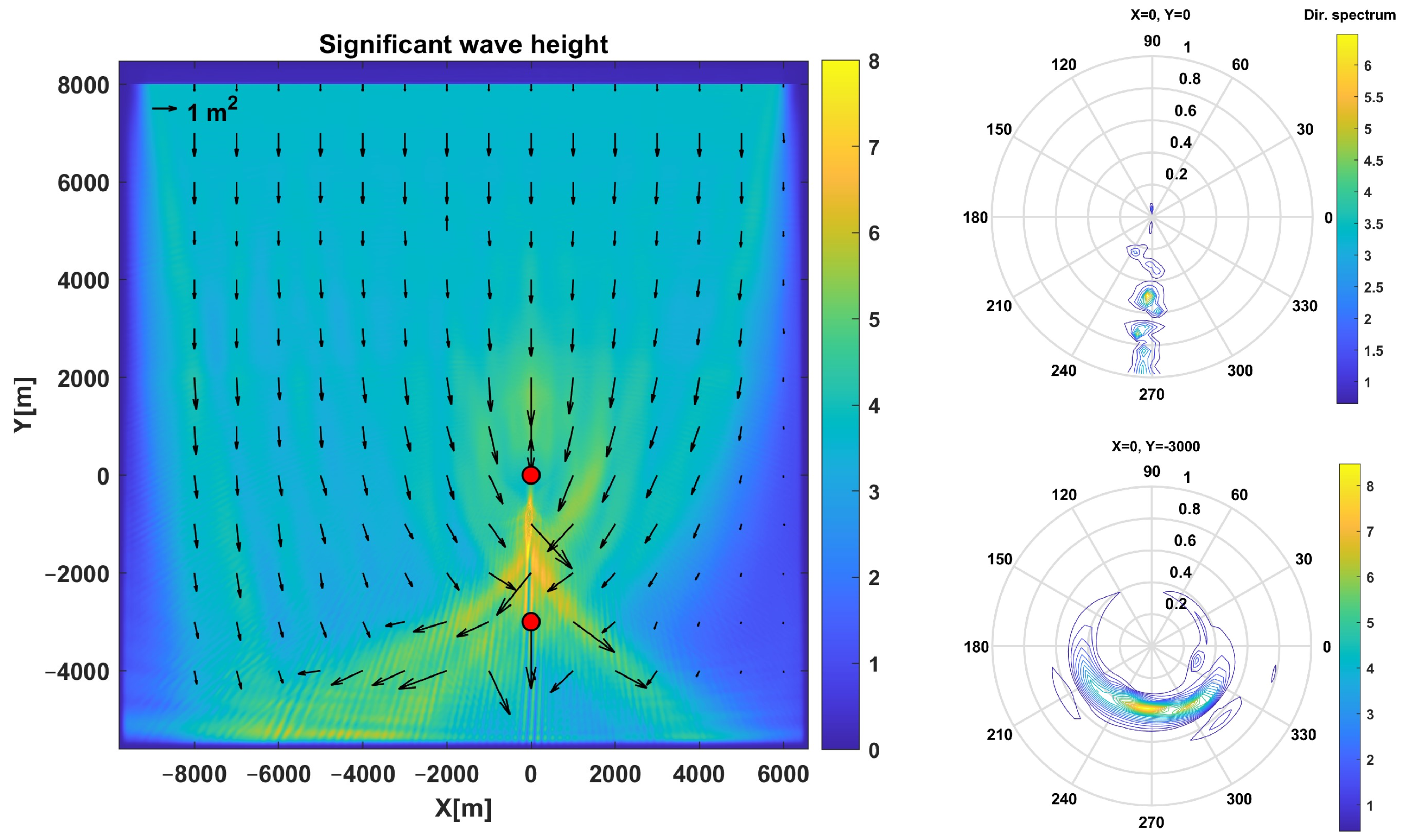
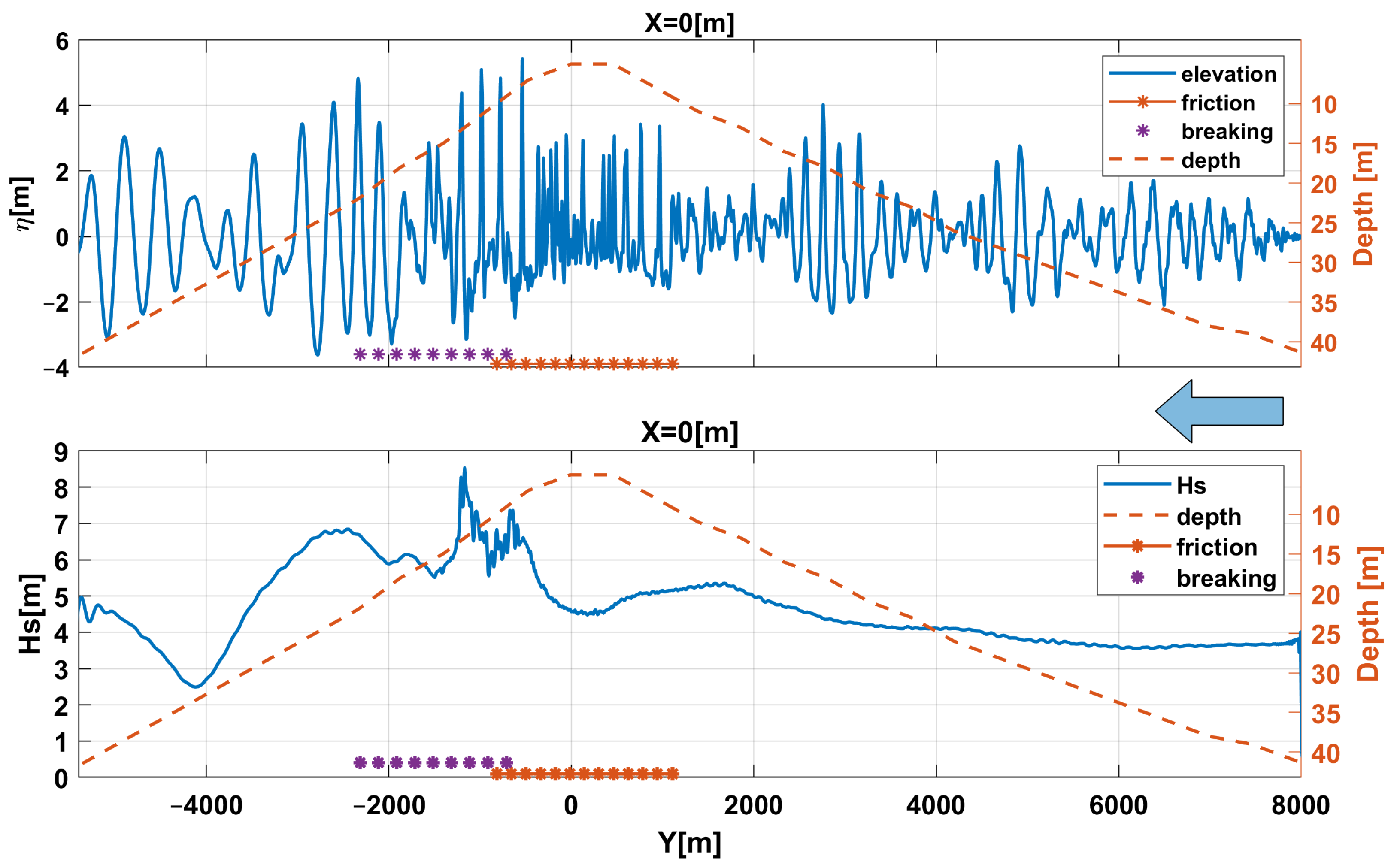
3. Case 1: Waves over the Glagah Seamount to the Coast

3.1. Domain and Numerical Setting
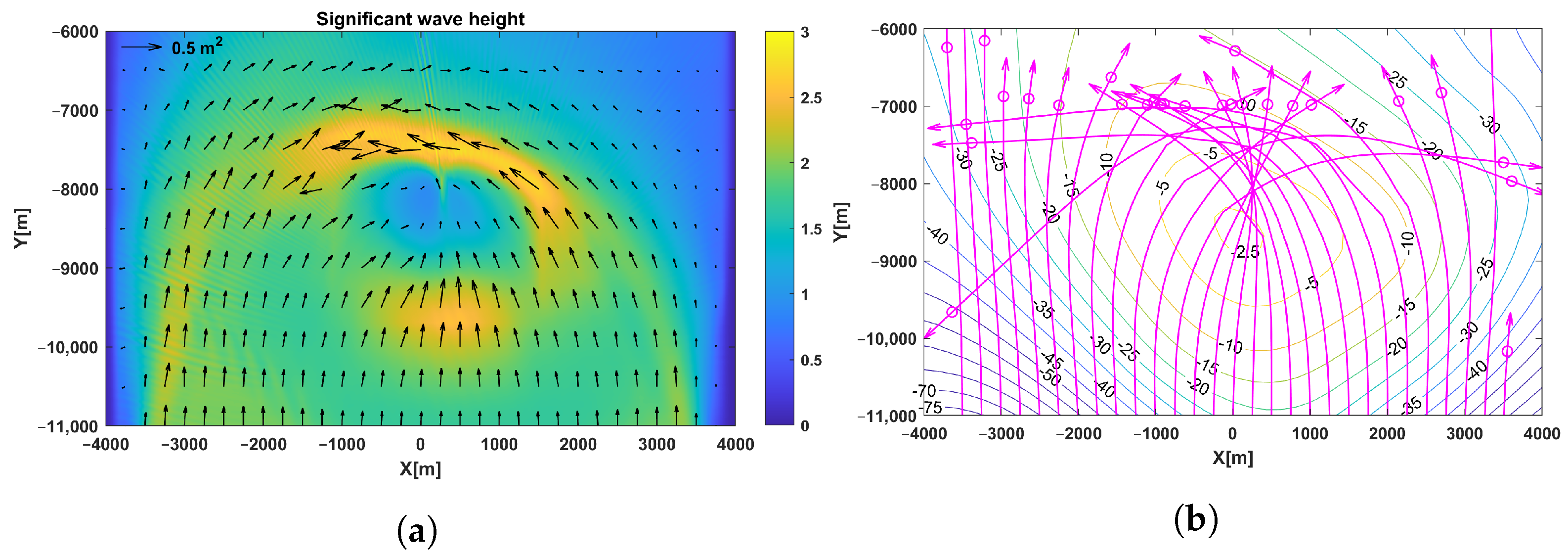
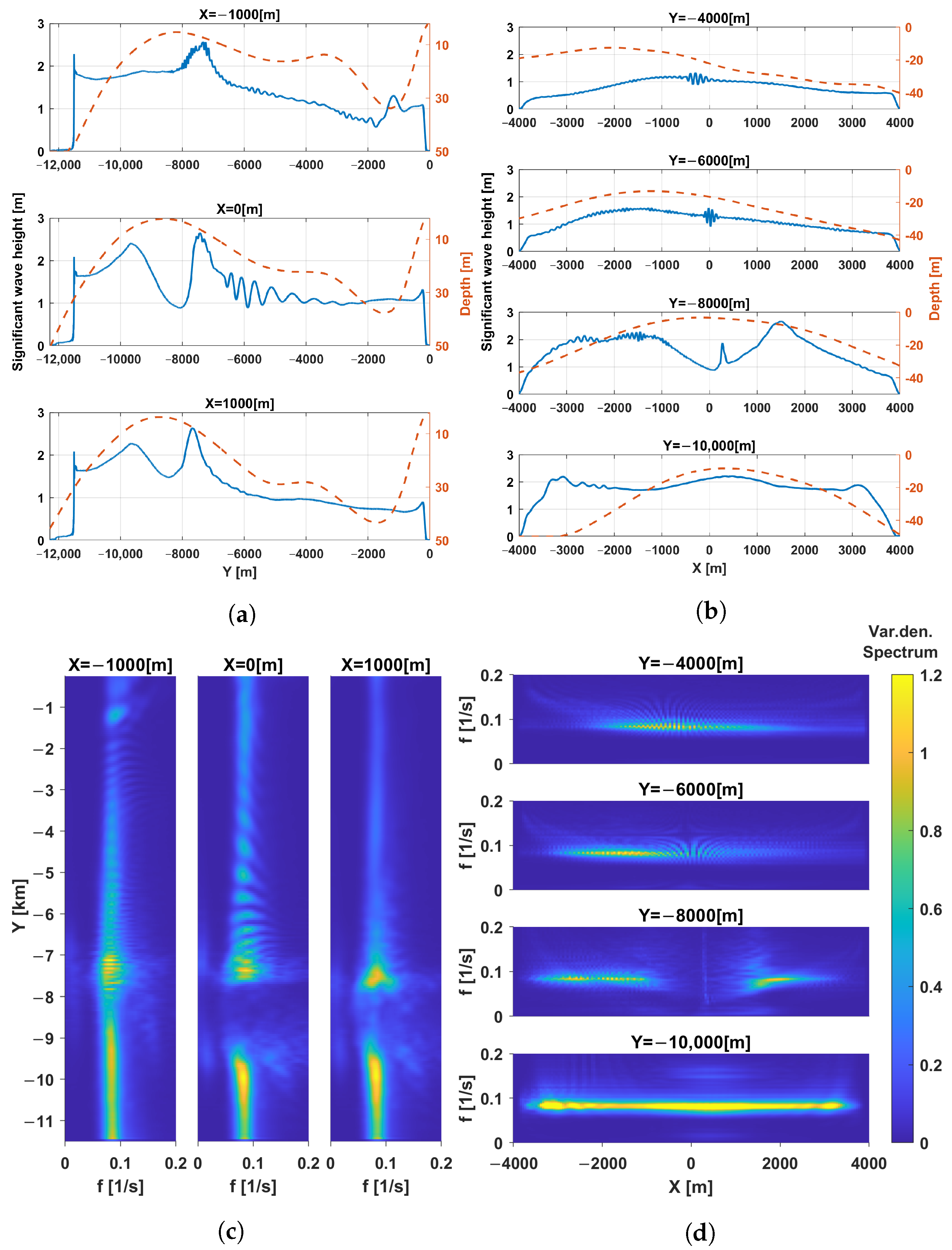
The topography map from the Indonesian Geospatial Information Agency BIG (https://tanahair.indonesia.go.id/portal-web/, accessed on 1 November 2021) in Figure 2 shows the top of the seamount some 8 km seaward of a small harbor, Glagah Port, that will serve as the origin of the coordinate system, ( x , y ) = ( 0 , 0 ) . To consider the environmental wave input in the main prevailing wave direction from southwest to the coastline, a rotation of about 23 degrees counter-clockwise is applied, as illustrated in Figure 2; the chosen simulation domain then extends about 8 km along the coastline and 12 km seaward from the coastline. After the rotation, the domain is described with x ( 4000 , 4000 ) m in the direction along the coast and y (−12,500, 0) m perpendicular to the coastline. The seamount is near ( x , y ) = ( 0 , 8500 ) m in the simulation domain. In the direction from bottom to top, the bathymetry over the cross-section through the top increases from a depth of 60 m to 2 m at the top, followed by a decrease to nearly 40 m, and then increases to the shoreline. The converging and diverging level lines are expected to cause substantial diffraction and refraction.
The choice of the orientation of the domain is partly determined by the dominant wave direction from the ocean in the area, but partly also for numerical reasons, to reduce the realistic energy outflow through the boundaries as much as possible. To prevent periodic looping, damping zones with widths of 296 m are added along all boundaries; therefore, outgoing waves will reduce the total energy in the area without compensation for incoming waves from outside the simulation area.
Referring to the bathymetry plot in Figure 2, we used the rotated domain with a total area of 96 km 2 that is covered by a grid with a size of 4 m in the x-direction and y-direction, resulting in 2048 × 3072 grid points in the simulation domain. Waves were simulated over a total time of 4800 s, in which the main waves fill the domain and reach the coastal area in approximately 20 min; all statistical quantities are calculated for the last 3600 s.
The influx properties are determined by a Jonswap spectrum with γ = 3.3 , peak period T p = 12 s or wave frequency f = 0.083 Hz, and significant wave height H s = 2 m. The waves are influxed without spreading along the line that has a length of −7600 m, x ( 3800 , 3800 ) m at y = −11,500 m. We applied damping boundary conditions so that the outflow smoothly vanishes at all boundaries. The damping zones along the domain boundary have a width of 296 m. We used bottom friction with the coefficient F = 0.05 around the seamount x ( 1100 , 1500 ) m, y ( 9700 , 7400 ) m.

3.2. Wave Elevation

In this section, we present the numerical wave simulation results over the whole domain and zoom in near the seamount. Figure 3a gives a snapshot view of the wave elevation at a time of 2400 s, while Figure 3b shows the significant wave height with contour levels of the bathymetry. The zoomed versions are presented in Figure 3b,c. The significant wave height from the numerical simulation is computed from the surface wave elevation H s = 4 σ , where σ is the standard deviation of the surface wave elevation. The highest significant wave height is 2.97 m, i.e., 1.49 times the influx H s , near ( x , y ) = ( 188 , 7432 ) downstream of the seamount.
The depth contour lines, as shown in Figure 3b, and Fermat’s principle guide the understanding of the energy propagation over the area. From the influx at the bottom, the bent contour lines will cause the waves to focus strongly and embrace the mount. As the waves approach the top of the seamount, waves from the sides of the simulation domain are refracted strongly toward the top. Because there is no influx from the left (and right) vertical boundary in the simulation downstream to the west of the mount, the waves nearly vanish and are small towards the east. This creates, at the west side, an area towards the beach with very few waves, so that the effects of a second mount with a top of 10 m below the surface at (−2000, −3000) is hardly noticeable. From Figure 3b, we also observe that the significant wave height H s shows substantial changes due to depth differences; for instance, the value of H s = 1 m at the top of the seamount is only one-third of the value in the ring-shaped yellow area that is caused by strong diffracting surrounding waves.
Figure 4 shows snapshots of the waves moving from deep water toward the coast (left to right) over three cross-sections, at x = 1000 , 0 , and 1000 m. The wave elevation at a certain time already shows the wavelength changes due to the seamount; shorter waves are generated when waves approach the top of the seamount.

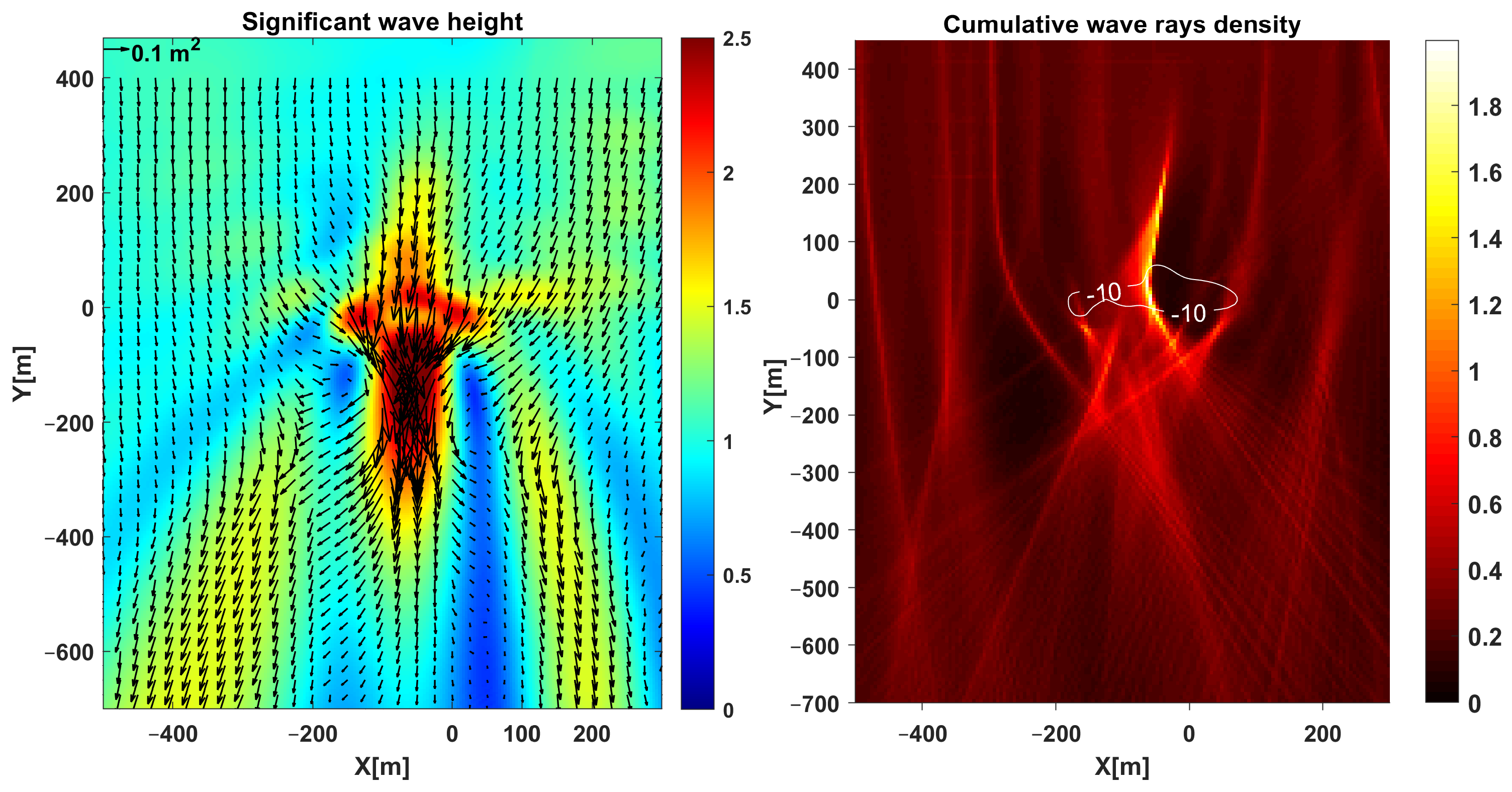
3.3. Main Wave Directions (Wave Rays)

The numerical simulation in Figure 5a describes the main wave direction near the seamount computed from the wave spectrum roses. The length of the vector indicates the wave’s potential energy, V a r ( η 2 ) , proportional to the significant wave height, which is also spatially presented as the background color. Meanwhile, Figure 5b shows the analytical wave ray tracing for comparison. The plots show that the seamount acts like a convex lens in optics, where incoming light waves are focused on a focal point behind it. The wave tracing shown in Figure 5b is obtained by applying Snell’s law based on the wave group velocity at peak frequency. The theoretical ray tracing starts by calculating at each point of the domain the group velocity V ( x , y ) from the local peak wave frequency and depth [38]. For the chosen contour spacing d V , contour lines of the group velocity are determined, and the averaged value between two successive contour lines provides the discretized V ( x , y ) . For the given initial position and propagation direction, at each ray-crossing, the propagation direction is adjusted according to Snell’s Law; for the velocity spacing d V , we took 1% of the maximum group speed, approximately 0.1 m/s.

3.4. Wave Spectra

The wave transformation over the Glagah seamount can also be investigated from the changes in the wave spectra. Figure 6c,d shows the 2D wave spectra corresponding to the significant wave height in Figure 6a,b.
Observe from Figure 6 the initially large significant wave height drops to a value of H s = 1 m over the top of the seamount. Even though the waves converge to the summit, the wave shoaling process is limited by the water depth. The low wave height over the shallowest area occurs because of the diffraction and the energy dissipation. The waves then develop a focusing area downstream by a strong refraction process. While we observed significant changes along the x-cross-sections, the waves along the y-cross-sections do not differ so much, except the cross-section over the top. The cross-section at y = 8500 m shows decreasing waves over the summit.
Each plot aims to portray the transformation of the waves in the spatial and frequency domains. Along the line, it not only presents the peak frequency of the waves, but it also exhibits the changes in the distribution of the energy spectral density over the frequency domain. Looking at the spectrum over the vertical line through the top of the seamount ( x = 0 m) (Figure 6c,d), a broadening of the spectrum occurs just before the top, showing the development of short waves and infra-gravity waves during wave shoaling.
Over the top of the seamount, there are no high-energy density spectra, showing that the waves lose energy. Some distance further in the direction of the coast, waves from the sides merge and become visible in the spectrum. From Figure 6d, the wave spectrum along y = −10,000 m still has the same peak frequency with a similar distribution of the energy density, while along y = 8500 m, the waves are only prominent to the sides of the seamount. The gaps in the spectra indicate that the waves transform to a flow towards the top of the seamount; after passing it, undulations grow and transform into down-running waves. After crossing the top of the seamount, the wave spectrum at y = 6000 m describes refracted waves with less energy than the influx, which then run-down in a nearly waveless flow. Less energy reaches the coast due to the dissipation of energy over the top of the seamount and also due to energy outflow through the domain boundaries.

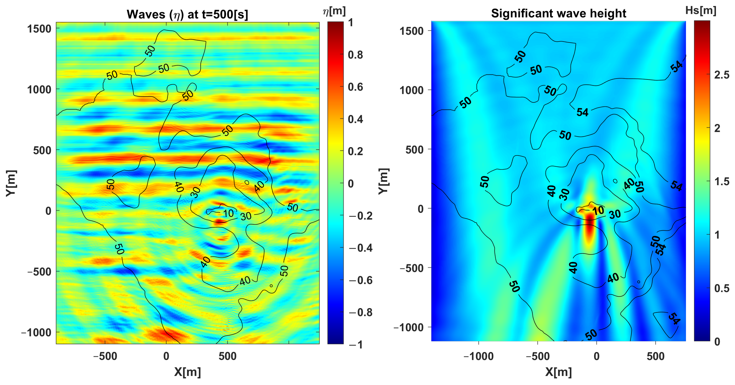
4. Case 2: Waves over the Socotra Rock

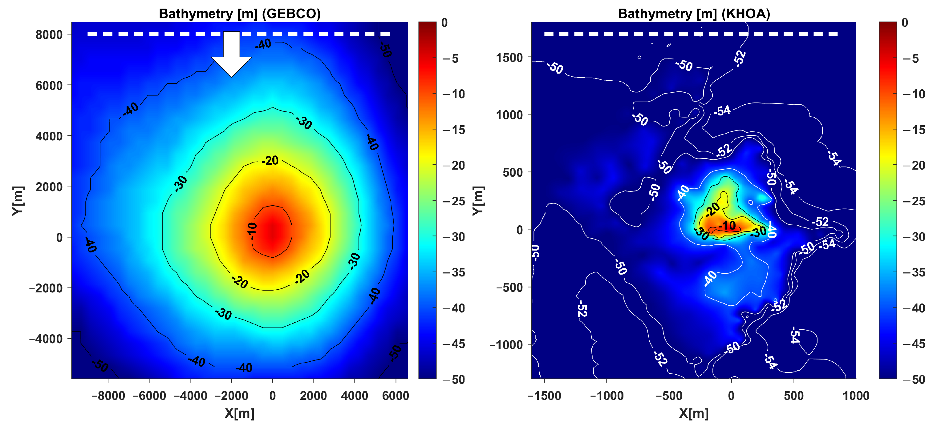
4.1. Domain and Numerical Setting

As a second case, we show results for waves over the Socotra Rock, south of Korea in the East China Sea, with a top 4.6 m under the sea surface, surrounded by 60 m deep water. The rock has a research station with an observation platform; see [39], https://en.wikipedia.org/wiki/Ieodo_Ocean_Research_Station (accessed on 1 November 2021). Simulations with input determined by a Jonswap spectrum are presented in this section to show the deformation of phase-resolved waves over an area of 16 km × 14 km (224 km 2 ). For wave influx, the wave direction distribution is taken from the platform data over one year (March 2021–March 2022), during which most waves propagated from north to south. The selection of the main wave direction and the peak periods is based on the wave data distribution over one year. Waves from the north are simulated above the bathymetry in the large and small domains shown in Figure 7. The domains, with the top of the seamount positioned at the origin (0, 0), are chosen to reduce energy outflow through the boundaries as much as possible. In both the large and small domains, damping boundary conditions are applied, with a width of 200 m as a damping zone along all sides.
For the Socotra Rock case, we conduct two simulations. The first simulation is in a large domain with bathymetry data obtained from the General Bathymetric Chart of the Oceans (GEBCO). The simulation uses a grid size of 8 m in the x- and y-directions (1320 × 1280 grid points) with a friction value of 0.05 applied at depths less than 10 m where the bottom is assumed to be mostly rock at shallower depths. In deeper water, we do not in include friction, to prevent more energy loss approaching the top of the seamount. Wave influx without directional spreading is generated from the north at y = 8000 m to the south. The wave has a typical Jonswap spectrum with T p = 15 s and H s = 4 m for a duration of 80 min (the main wave takes approximately 20 min to fill the area). Looking at the bathymetry changes above Socotra, the waves from the north are expected to converge to the summit. We expect the waves will converge more if we choose no spreading wave as the influx. The expected focusing wave will be higher as it spreads less than the real one.
The second simulation is conducted in a smaller domain (2.5 km by 3 km) using high-resolution bathymetry data obtained from an in situ 2017 survey by the Korea Hydrographic and Oceanographic Agency (KHOA), which is available at http://www.khoa.go.kr/oceanmap/main.do (accessed on 1 November 2021). The domain is x ( 1600 , 959 ) , y ( 1320 , 1796 ) , with damping zones of 200 m along the boundaries. Different from the large domain’s bathymetry that changes smoothly, the bathymetry in the smaller domain changes abruptly. Waves with a large significant wave height will become much steeper and mostly break. To avoid a chaotic wave condition and focus on details of the waves around the rock, a smaller wave height will be chosen for the simulation. Therefore, for wave influx from the north at y = 1580 m, Jonswap spectra are used with significant wave height H s = 1 m, peak wave period T p = 15 s, peak enhancement factor γ = 3.3 , and no directional spreading.

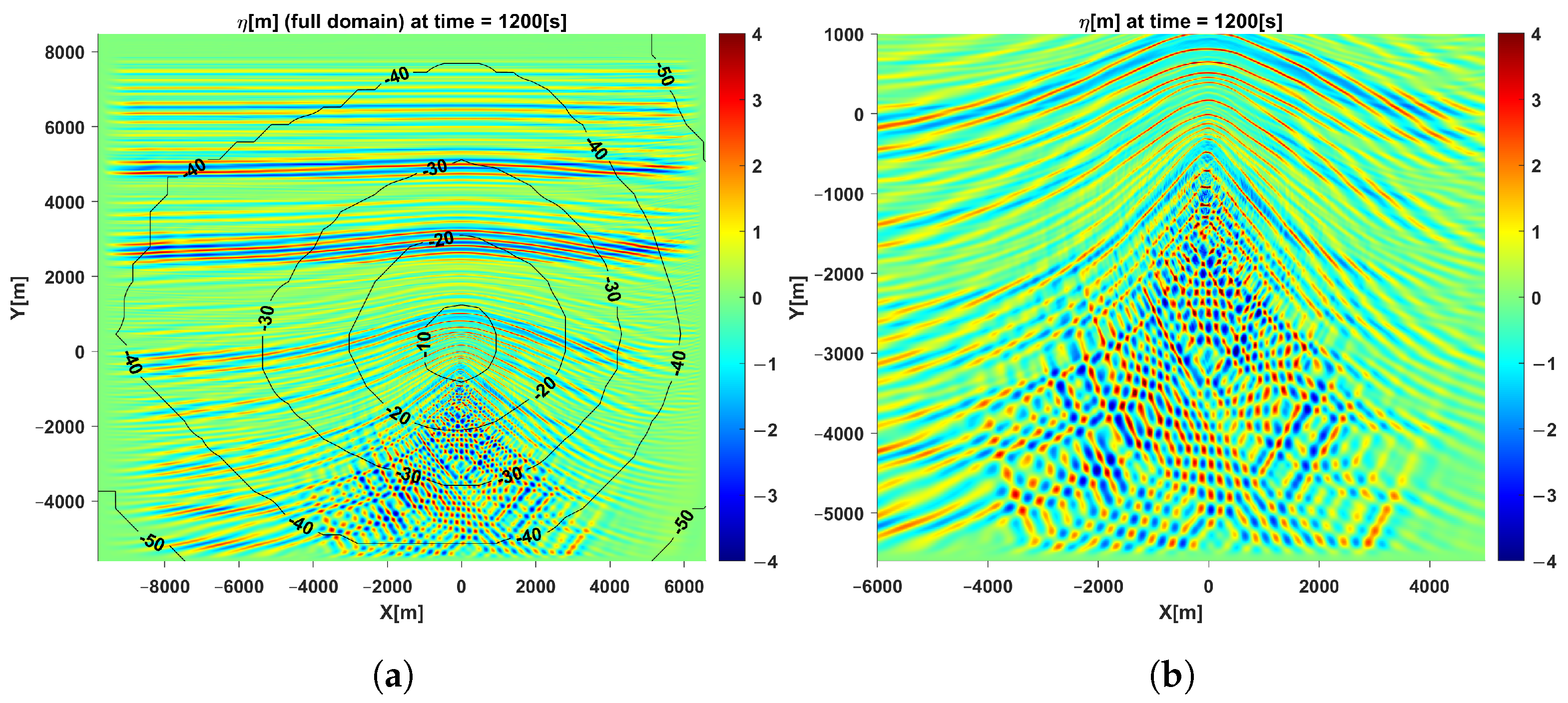
4.2. Waves over the Large Domain (GEBCO)

The snapshot of the wave elevation at t = 1200 s in Figure 8a,b shows a very different pattern between the upstream and downstream regions of the seamount. Interference of the refracted waves downstream of the mount creates a characteristic cross sea, as shown in Figure 8. The cross seas are observed from the wave direction in Figure 9 (left), showing the waves from the right turn to the left and vice versa after passing the mount. The directional spectrum at the mount and downstream in Figure 9 (right) also presents how strong the refraction waves are after crossing the mount; incoming waves with no spreading transform into waves with very wide spreading and turn to crossing waves in the wake of the Socotra Rock.
Figure 10 presents a snapshot of the wave elevation and the significant wave height at t = 1200 s along the top of the mount cross-section. The wavelength changes are observed in the upper plot of Figure 10; short waves appear on top of the mount, while longer waves are observed downstream. A lower wave amplitude over the top also results from friction. We observe peaks before and after the seamount from the significant wave height presented in the lower plot of Figure 10. The first peak before the top is caused by wave shoaling, while the strong wave refraction causes the second peak after the top.

4.3. Waves around the Rock (KHOA)

Unlike the bathymetry used in the large-domain simulation that is mostly ideal circular, the high-resolution bathymetry around the rock is relatively complex with quite steep rock. Therefore, the wave elevation in Figure 11 (left) shows that the crossing sea pattern downstream is less visible here. Waves from the north over the Socotra Rock show strong refraction effects creating focusing waves downstream. The incoming waves with a significant wave height of 1 m develop a focusing wave with a significant wave height up to almost three times that after passing the top of the seamount; see Figure 11 (right).
The zoomed version of the significant wave height in Figure 12 (left) shows the wave shoaling phenomenon when waves approach the top; the decreasing depth up to the top amplifies the wave. Further, the wave amplification is much more significant due to the wave refraction. The simulated and theoretical directional patterns in Figure 12 show a large focusing area with denser arrows, indicating that waves collectively merge into higher waves downstream of the summit, followed by a gradual decrease further downstream. Consequently, flanks are also generated on both sides of the focusing region.
Figure 13 (top) shows the wave elevation at t = 5100 s, while the bottom panel shows the changes in H s over a cross-section passing the focusing point. Like the large-domain simulation results, waves from the north generate at least two local peaks. The wave shoaling generates the first peak when waves approach the top. The second peak, which is much larger, is generated by strong wave refraction behind the top of the seamount.

5. Discussion

Collecting measurement data over seamounts is a challenging task. So, numerical models are invaluable tools to give insight into the expected wave transformations due to the interactions between the surface wave and the seamount. Numerical wave simulations are, therefore, commonly conducted prior to experiments in the field or laboratory, which require more resources. Here, we studied the interactions between surface waves and the seamounts Glagah and Socotra Rock. The validation of the simulations near the seamounts is out of the study scope. Nevertheless, the summary of the model verification sufficiently justifies the model we used.
The numerical wave simulations over Glagah and Socotra Rock show similar physical processes, such as wave shoaling, diffraction–refraction, and shadowing effects downstream. The bathymetry data from GEBCO and KHOA used in the Socotra Rock simulations differ significantly. The GEBCO bathymetry is mostly an ideal circular bathymetry, in which the distance between the top of the seamount to 40 m depth is approximately 5 km, while it is only 500 m in the KHOA data. This different steepness of the slope leads to a different wave transformation. The generated crossing sea in the simulation using GEBCO could cover an area of several kilometers, while the crossing sea over KHOA only covers a small area. The steeper bathymetry in the simulation using KHOA makes the generated downstream focusing wave up to three times the input wave height. In contrast, the maximum significant wave height in the simulation using GEBCO is only two times the input. Compared to the Socotra case, the Glagah bathymetry is less steep, and the amplification is only 1.5 times the input wave.
This study has complemented the work of [40] that simulated the long-crested waves over a cross-section of Glagah. The long-crested wave simulations do not capture the physical wave deformations of diffraction–refraction that are essential in the area near the seamount. The lack of wave diffraction and refraction brings a less reliable approximation of the waves near the shore in the shadow area of the seamount. Here, we presented the importance of diffraction–refraction in the wave transformations over Glagah seamount and Socotra Rock. The numerical wave simulation over Socotra Rock conducted by [3] was based on a phase-averaged wave model. They observed the refraction from the asymmetrical distribution of the significant wave height; downstream wave heights were lower than the input wave. In this study, the refraction is directly observable from the wave rays, in agreement with the wave direction shown in [13]. The coarse resolution in [3] may lead to missing wave-refracted rays. Moreover, the unresolved wave would not show clearly the crossing sea right after the summit, as presented in our study.
In addition, the diffraction–refraction due to the seamount determines the focusing wave and the shadow zone downstream. The seamount acts like a convex lens as the refractive processes alter the incoming waves similarly [13]. The shadowing effect has been shown as being characteristic of a wave’s interaction with an obstacle. The shadow zone is clearly observed in both the Glagah and Socotra cases. The numerical phase-averaged model could also reveal this characteristic as well [3,13]. Similar phenomena have been found to be not only caused by seamounts but also in wind farms’ fields [41] and in swell simulations around islands [42].
In addition to the advantages of the phase-resolved wave model in showing most physical aspects of wave transformation, the model is still computationally demanding as it requires a fine grid to present the wave details. The numerical computation of the phase-resolved wave simulation by [16] took 5–10 times the length of the simulated time period. Even though the HAWASSI model has been claimed as an accurate and efficient model, especially the one-dimensional model, the simulation in two dimensions over a large-scale domain is still less practical unless we reduce the resolution. In this study, the computation time of the wave simulation mainly depends on the grid size. In the simulation of the Socotra Rock in the small domain (with 640 × 780 grid points), the computation takes approximately 23 h for an hour of simulation time. It would be only five hours if we reduced the grid to half of the origin, as the computation time is approximately linearly proportional to the grid size. Optimizing the model solver to reduce the computational cost would make the model more practical for forecasting applications.

6. Conclusions

This paper presents numerical phase-resolved wave simulations over two shallow seamounts. The detailed results in both cases show that the mounts act like an optical lens, refracting and diffracting the waves considerably, leading to wave crossing downstream of the summit. Two local maxima before and after the summit always occur because of the seamount, shoaling, and refraction phenomena. The direct decrease in the water depth amplifies the wave amplitude and creates a local maximum before the summit. Over the summit, waves dissipate energy because of the breaking and bottom friction effect. Even though the waves lose energy over the summit, wave refraction merges the waves from the right and left of the seamount into another focusing area behind the summit, accompanied by a wake zone ahead. The contour line in Socotra Rock makes the strong refraction from the right and left almost give the same energy; thus, a noticeable cross sea in deeper water is developed downstream of the rock.
In the isolated Glagah seamount, the wave transformations are observed further towards the coast. Towards the coast, a confused sea will result in noticeable effects on waves until the coastline. Although the bathymetry is nearly the same along the coast until a depth of 30 m, the incoming wave energy shows large variations because the mount substantially perturbs the wave directions and determines the waves near the coastline. Therefore, simulations with a sufficiently large domain are required to support structural designs and coastal safety investigations. Improvement and optimization of the model and validation should be considered for more practical applications. Reducing the model’s limitations in the complex breaking phenomena and bottom friction effect would be challenging. Nevertheless, this study provides insights into the detailed wave characteristics of the interactions between surface waves and obstacles in real fields.

Author Contributions

Conceptualization: E.v.G. and A.L.L.; theory: E.v.G. and D.H.; simulations: A.L.L., H.L.H., and D.H.; writing and editing: E.v.G. and A.L.L.; supervision: E.v.G. All authors have read and agreed to the published version of the manuscript.

Funding

This research received no external funding.

Institutional Review Board Statement

Not applicable.

Informed Consent Statement

Not applicable.

Data Availability Statement

The data that support the findings of this study are available from the corresponding author, A.L.L., upon request.

Acknowledgments

We acknowledge the Indonesian National Research and Innovation Agency for the High-Performance Computing facility and thank the Geospatial Information Agency of Indonesia for providing the bathymetry data used in this study.

Conflicts of Interest

The authors declare no conflict of interest.

References

  1. Nam, S.; Kim, D.J.; Lee, S.W.; Kim, B.G.; Kang, K.M.; Cho, Y.K. Nonlinear internal wave spirals in the northern East China Sea. Sci. Rep. 2018, 8, 3473. [Google Scholar] [CrossRef]
  2. Kim, S.-S.; Wessel, P. New global seamount census from altimetry-derived gravity data. Geophys. J. Int. 2011, 186, 615–631. [Google Scholar] [CrossRef]
  3. Sosa, J.; Cavaleri, L.; Portilla-Yandún, J. On the interaction between ocean surface waves and seamounts. Ocean Dyn. 2017, 67, 1553–1565. [Google Scholar] [CrossRef]
  4. Brink, K.H. A Comparison of Long Coastal Trapped Wave Theory with Observations off Peru. J. Phys. Oceanogr. 1982, 12, 897–913. [Google Scholar] [CrossRef]
  5. Brink, K. The effect of stratification on seamount-trapped waves. Deep Sea Res. Part A Oceanogr. Res. Pap. 1989, 36, 825–844. [Google Scholar] [CrossRef]
  6. Niu, X.; Yu, X. Analytic solution of long wave propagation over a submerged hump. Coast. Eng. 2011, 58, 143–150. [Google Scholar] [CrossRef]
  7. Haidvogel, D.B.; Beckmann, A.; Chapman, D.C.; Lin, R.Q. Numerical Simulation of Flow around a Tall Isolated Seamount. Part II: Resonant Generation of Trapped Waves. J. Phys. Oceanogr. 1993, 23, 2373–2391. [Google Scholar] [CrossRef]
  8. Stashchuk, N.; Vlasenko, V. Internal Wave Dynamics Over Isolated Seamount and Its Influence on Coral Larvae Dispersion. Front. Mar. Sci. 2021, 8, 735358. [Google Scholar] [CrossRef]
  9. Zhang, L.; Buijsman, M.C.; Comino, E.; Swinney, H.L. Internal wave generation by tidal flow over periodically and randomly distributed seamounts. J. Geophys. Res. Ocean. 2017, 122, 5063–5074. [Google Scholar] [CrossRef]
  10. Chapman, D.C.; Haidvogel, D.B. Formation of Taylor caps over a tall isolated seamount in a stratified ocean. Geophys. Astrophys. Fluid Dyn. 1992, 64, 31–65. [Google Scholar] [CrossRef]
  11. Perfect, B.; Kumar, N.; Riley, J.J. Vortex Structures in the Wake of an Idealized Seamount in Rotating, Stratified Flow. Geophys. Res. Lett. 2018, 45, 9098–9105. [Google Scholar] [CrossRef]
  12. Perfect, B.; Kumar, N.; Riley, J.J. Energetics of Seamount Wakes. Part I: Energy Exchange. J. Phys. Oceanogr. 2020, 50, 1365–1382. [Google Scholar] [CrossRef]
  13. Biolchi, L.G.; Farina, L.; Perotto, H. The influence of seamounts on ocean surface wave propagation in Northeast Brazil. Deep Sea Res. Part I Oceanogr. Res. Pap. 2020, 156, 103185. [Google Scholar] [CrossRef]
  14. Thomas, T.J.; Dwarakish, G. Numerical Wave Modelling—A Review. Aquat. Procedia 2015, 4, 443–448. [Google Scholar] [CrossRef]
  15. Fergstad, D.; Økland, O.; Stefanakos, C.; Stansberg, C.T.; Croonenborghs, E.; Eliassen, L.; Eidnes, G. LFCS Review Report—Environmental Conditions; Technical Report; SINTEF Ocean: Trondheim, Norway, 2018. [Google Scholar]
  16. Wang, W.; Pákozdi, C.; Kamath, A.; Bihs, H. Fully nonlinear phase-resolved wave modelling in the Norwegian fjords for floating bridges along the E39 coastal highway. J. Ocean Eng. Mar. Energy 2023, 9, 567–586. [Google Scholar] [CrossRef]
  17. Buckley, M.; Lowe, R.; Hansen, J. Evaluation of nearshore wave models in steep reef environments. Ocean Dyn. 2014, 64, 847–862. [Google Scholar] [CrossRef]
  18. Junwoo, C. Numerical Simulations of Rip Currents Under Phase-Resolved Directional Random Wave Conditions. J. Korean Soc. Coast. Ocean Eng. 2015, 27, 238–245. [Google Scholar] [CrossRef]
  19. Henderson, C.S.; Fiedler, J.W.; Merrifield, M.A.; Guza, R.; Young, A.P. Phase resolving runup and overtopping field validation of SWASH. Coast. Eng. 2022, 175, 104128. [Google Scholar] [CrossRef]
  20. Nguyen, Q.T.; Mao, M.; Xia, M. Numerical Modeling of Nearshore Wave Transformation and Breaking Processes in the Yellow River Delta with FUNWAVE-TVD Wave Model. J. Mar. Sci. Eng. 2023, 11, 1380. [Google Scholar] [CrossRef]
  21. Zakharov, V.E. Stability of periodic waves of finite amplitude on the surface of a deep fluid. J. Appl. Mech. Tech. Phys. 1972, 9, 190–194. [Google Scholar] [CrossRef]
  22. Broer, L.J.F. On the hamiltonian theory of surface waves. Appl. Sci. Res. 1974, 29, 430–446. [Google Scholar] [CrossRef]
  23. Kurnia, R.; van Groesen, E. High order Hamiltonian water wave models with wave-breaking mechanism. Coast. Eng. 2014, 93, 55–70. [Google Scholar] [CrossRef]
  24. van Groesen, E.; van der Kroon, I. Fully dispersive dynamic models for surface water waves above varying bottom, Part 2: Hybrid spatial-spectral implementations. Wave Motion 2012, 49, 198–211. [Google Scholar] [CrossRef]
  25. She Liam, L.; Adytia, D.; van Groesen, E. Embedded wave generation for dispersive surface wave models. Ocean Eng. 2014, 80, 73–83. [Google Scholar] [CrossRef]
  26. Bühler, O.; Jacobson, T.E. Wave-driven currents and vortex dynamics on barred beaches. J. Fluid Mech. 2001, 449, 313–339. [Google Scholar] [CrossRef]
  27. Kennedy, A.B.; Chen, Q.; Kirby, J.T.; Dalrymple, R.A. Boussinesq Modeling of Wave Transformation, Breaking, and Runup. I: 1D. J. Waterw. Port Coast. Ocean Eng. 2000, 126, 39–47. [Google Scholar] [CrossRef]
  28. Kurnia, R.; van Groesen, E. Spatial-spectral Hamiltonian Boussinesq wave simulations. In Advances in Computational and Experimental Marine Hydrodynamics (ACEMH 2014); IIT Madras: Chennai, India, 2014. [Google Scholar]
  29. Kurnia, R.; van den Munckhof, T.; Poot, C.P.; Naaijen, P.; Huijsmans, R.H.M.; van Groesen, E. Simulations for Design and Reconstruction of Breaking Waves in a Wavetank. In Proceedings of the ASME 2015 34th International Conference on Ocean, Offshore and Arctic Engineering, St. John’s, NL, Canada, 31 May–5 June 2015; Volume 1. [Google Scholar] [CrossRef]
  30. Kurnia, R.; van Groesen, E. Localization for spatial–spectral implementations of 1D Analytic Boussinesq equations. Wave Motion 2017, 72, 113–132. [Google Scholar] [CrossRef]
  31. Latifah, A.L.; Handri, D.; Shabrina, A.; Hariyanto, H.; van Groesen, E. Statistics of Simulated Storm Waves over Bathymetry. J. Mar. Sci. Eng. 2021, 9, 784. [Google Scholar] [CrossRef]
  32. Kurnia, R.; Badriana, M.R.; van Groesen, E. Hamiltonian Boussinesq Simulations for Waves Entering a Harbor with Access Channel. J. Waterw. Port Coast. Ocean Eng. 2018, 144, 04017047. [Google Scholar] [CrossRef]
  33. Kurnia, R.; Turnip, P.; van Groesen, E. Spectral AB Simulations for Coastal and Ocean Engineering Applications. In Proceedings of the Fourth International Conference in Ocean Engineering (ICOE2018); Murali, K., Sriram, V., Samad, A., Saha, N., Eds.; Springer: Singapore, 2019; pp. 207–217. [Google Scholar]
  34. van Groesen, E.; Andonowati. Hamiltonian Boussinesq formulation of wave–ship interactions. Appl. Math. Model. 2017, 42, 133–144. [Google Scholar] [CrossRef]
  35. Bouscasse, B.; Ducrozet, G.; Kim, J.W.; Lim, H.; Choi, Y.M.; Bockman, A.; Pakozdi, C.; Croonenborghs, E.; Bihs, H. Development of a Protocol to Couple Wave and CFD Solvers Towards Reproducible CFD Modeling Practices for Offshore Applications. In Proceedings of the ASME 2020 39th International Conference on Ocean, Offshore and Arctic Engineering, Virtual, 3–7 August 2020. [Google Scholar]
  36. Kim, J.; Jang, H.; Lim, H.J.; Lai, L.; Latifah, A.; Auburtin, E.; Tcherniguin, N.; Petrie, F. Numerical Ocean Wave-Basin (NOW): A Numerical Solution for FSRU Mooring Design Analysis. In Proceedings of the ASME 2021 40th International Conference on Ocean, Offshore and Arctic Engineering, Virtual, 21–30 June 2021; Volume 1, p. V001T01A034. [Google Scholar] [CrossRef]
  37. Fouques, S.; Croonenborghs, E.; Koop, A.; Lim, H.J.; Kim, J.; Zhao, B.; Canard, M.; Ducrozet, G.; Bouscasse, B.; Wang, W.; et al. Qualification Criteria for the Verification of Numerical Waves—Part 1: Potential-Based Numerical Wave Tank (PNWT). In Proceedings of the SME 2021 40th International Conference on Ocean, Offshore and Arctic Engineering, Virtual, 21–30 June 2021. [Google Scholar]
  38. Waltham, D.A. Two-point ray tracing using Fermat’s principle. Geophys. J. 1988, 93, 575–582. [Google Scholar] [CrossRef]
  39. Kim, B.-N.; Jung, S.-K.; Choi, B.K.; Km, B.-C.; Shim, J. Long-term observation of underwater ambient noise at the Ieodo Ocean Research Station in Korea. In Proceedings of the 2015 IEEE Underwater Technology (UT), Chennai, India, 23–25 February 2015; pp. 1–3. [Google Scholar] [CrossRef]
  40. Latifah, A.; Shabrina, A.; Handri, D. Simulations of long-crested wind waves over the shallow seamount at Glagah. Appl. Ocean Res. 2022, 129, 103366. [Google Scholar] [CrossRef]
  41. Ponce de León, S.; Bettencourt, J.; Kjerstad, N. Simulation of irregular waves in an offshore wind farm with a spectral wave model. Cont. Shelf Res. 2011, 31, 1541–1557. [Google Scholar] [CrossRef]
  42. Humeniuk, J.F.; de León, S.P.; Violante-Carvalho, N.; de Carvalho, L.M.; Soares, C.G. Sheltering effect of islands on the Pacific swell. In Developments in Maritime Transportation and Exploitation of Sea Resources; CRC Press: London, UK, 2013. [Google Scholar]
Figure 1. Illustration of wave variables in x-direction. Free surface elevation η , surface tangential velocity v, water depth D, friction coefficient F, acceleration due to gravity g, wavelength λ , wave amplitude A, and wave height H. The red arrow illustrates the bottom friction.
Jmse 11 01765 g001
Figure 2. Simulation domain of case 1, in which the left plot is for waves from the southwest, rotated to show waves from bottom to top in the right plot. The black dashed lines are the boundaries of the simulation domain with a damping zone.
Jmse 11 01765 g002
Figure 3. (a) Wave elevation at t = 2400 s with the dashed line in the south showing the influx line. (b) The bathymetry level lines over the domain; the background color is determined by the significant wave height H s . (c,d) The zoomed versions of (a,b), respectively, near the seamount.
Jmse 11 01765 g003
Figure 4. Snapshots of the wave elevations at t = 2400 s on three vertical cross-sections (from top down at x = 1000 , 0 , 1000 m); the bathymetry is indicated with a dashed line with the depth on the right-hand axis.
Jmse 11 01765 g004
Figure 5. (a) Main wave directions near the seamount, in which the background color indicates the significant wave height and the vector length indicates the wave energy. (b) The wave trajectories constructed with Snell’s law at peak frequency.
Jmse 11 01765 g005
Figure 6. (a) H s along cross-sections x = 1000 , 0 , 1000 m with the bathymetry as a dashed line (right-hand axis), and (b) along y = −10,000, 8000 , 6000 , 4000 m. (c,d) The corresponding wave spectra.
Jmse 11 01765 g006
Figure 7. (left) Plot shows the bathymetry around Socotra Rock from GEBCO over the large-domain simulation with the dashed line represent the influx line and an arrow shows the wave influx diretion. (right) Plot shows the high-resolution bathymetry over the small-domain simulation.
Jmse 11 01765 g007
Figure 8. (a) Shows at t = 1200 s waves from the north creating a cross sea downstream of the mount shown in (b).
Jmse 11 01765 g008
Figure 9. (left) Plot shows the main wave directions with the value of H s as background. The length of the vector indicates the wave energy. (right) Plot shows the 2D spectra for the two positions indicated in the left plot.
Jmse 11 01765 g009
Figure 10. Wave elevation at a time of 1200 s (upper panel) and significant wave height (lower panel) over a cross-section ( x = 0 m). The intervals with the orange and purple stars represent the locations of the friction and the breaking, respectively. The dashed line indicates the bathymetry.
Jmse 11 01765 g010
Figure 11. A snapshot of the wave elevation at t = 5100 s (left) and the significant wave height (right). The contour lines in both plots shows the bathymetry.
Jmse 11 01765 g011
Figure 12. The significant wave height (left) with arrows representing the wave direction. (right) Plot shows the wave tracing using Snell’s Law with 10 m bathymetry level line.
Jmse 11 01765 g012
Figure 13. The upper plot shows the wave elevation over a cross-section ( x = 60 m) at t = 5100 s. The lower plot shows the significant wave height. The dashed line indicates the bathymetry.
Jmse 11 01765 g013
Disclaimer/Publisher’s Note: The statements, opinions and data contained in all publications are solely those of the individual author(s) and contributor(s) and not of MDPI and/or the editor(s). MDPI and/or the editor(s) disclaim responsibility for any injury to people or property resulting from any ideas, methods, instructions or products referred to in the content.

