Research on Ship Trajectory Prediction Method Based on Difference Long Short-Term Memory

Abstract

This study proposes a solution to the problem of inaccurate and time-consuming ship trajectory prediction caused by frequent ship maneuvering in complex waterways. The proposed solution is a ship trajectory prediction model that uses a difference long short-term memory neural network (D-LSTM). To improve prediction performance and reduce time dependence, the model combines the other variables of dynamic time features in the ship’s Automatic Identification System (AIS) data with nonlinear elements in the sequence data. The effectiveness of this method is demonstrated by comparing its accuracy to other commonly used time series modeling techniques. The results show that the proposed model significantly reduces training time and improves prediction accuracy.

1. Introduction

As an important component of global trade and transport, maritime traffic plays a key role in promoting international economic development and the progress of human civilization. However, with the growing number of ships and the complexity of the navigational environment, the management of maritime traffic is facing more and more challenges. The frequent occurrence of ship accidents and the increased risk of ship collision have brought great safety hazards to marine traffic. In order to ensure navigation safety, optimize ship routes, and improve the efficiency of marine traffic, ship trajectory prediction has become an important technical means of ensuring the safety of marine traffic and improving the efficiency of navigation.

1.1. Related Work

Ship trajectory prediction is primarily based on analyzing AIS data from past ship trajectories as well as environmental and other relevant factors to forecast future ship movements. This is an essential field of study that enhances the efficiency and safety of ship transportation. Domestic and international research on ship trajectory prediction can be grouped into various categories. The most common is the statistical model-based approach. With this method, probability or regression models are built using historical data for statistical analysis in order to forecast future ship paths. The mean, variance, and frequency distribution of the trajectory data can be calculated and used to create predictions. Typical statistical models include linear regression, the Kalman filter, and ARIMA (autoregressive integrated moving average). This approach typically presupposes specific correlations and patterns between potential future trajectories and past trajectories, and it captures these correlations and patterns through statistical analysis. It is mainly suitable for forecasting short- and small-range ship trajectories. Fan Jinghong [1] characterized the changing trend of ship positioning navigation and ship paths by incorporating big data technology into the mathematical model of ship positioning and trajectory prediction. The ship trajectory was predicted and smoothed using the Kalman filter approach by Xu et al. [2]. Jiang et al. [3] created an enhanced polynomial Kalman filter technique, with which one can obtain real-time estimation and prediction of a ship’s motion state by making up for missing information in the ship’s trajectory data. Using location, velocity, and direction to build a transfer matrix and a third-order Markov chain, Guo et al. [4] examined the impact of various parameters and orders on the uncertainty of ship trajectories. In order to apply the Gaussian process to describe the ship with lateral uncertainty and to predict the future position by probability, Rong et al. [5] divided the ship’s position into lateral and vertical parts. Qiao et al. [6] proposed a hidden Markov model that can adapt to the change in a ship’s speed and automatically select the corresponding parameters and extract the hidden and observed states from the trajectory data to determine the probability of state transfer to predict the ship’s position information, speed, and acceleration. Murray et al. [7] analyzed and investigated a data-driven approach to ship trajectory prediction using AIS data and proposed a single-point neighborhood search algorithm for ship trajectory prediction which predicts the next trajectory point by searching for the ship’s previous trajectories.

Methods based on classical machine learning: Through the learning and modeling of historical ship trajectory data, characteristics are derived and models are constructed to produce predictions. The engineering of the features of the data is initially required for this kind of technique; this entails choosing and extracting features relevant to trajectory prediction, such as position, speed, acceleration, heading, etc. Then, using several variables, including the ship’s navigation environment, the weather, the ship type, the crew experience, etc., the extracted characteristics are trained and learned using machine learning algorithms. The models can be decision trees, random forests, support vector machines, etc. By using equation constraints for support vector regression optimization and the particle swarm optimization approach to choose the best parameters to construct a least squares support vector regression model, Wang Jundang et al. [8] predicted trajectories. Mazzarella et al. [9] constructed a knowledge-based particle filtering (KB-PF) model for prediction. They provided the relevant confidence level by extracting features related to ship trajectory prediction using domain expert knowledge and combining it with conventional particle filtering (PF). In order to lessen the need for human involvement in trajectory prediction, Qi et al. [10] added characteristics relating to ship motion to the spatial clustering method and support vector machine classifier. In order to overcome the issues of uneven ship trajectory data and low similarity recognition, Jin [11] suggested an improved multiclassification logistic regression approach. The fuzzy C-mean (FCM) algorithm was used by Gan et al. [12] to segment historical trajectories and cluster them into smaller groups and then to weigh the clustered trajectories to determine predicted trajectory lengths in order to lower traffic signal mistakes in the Yangtze River. Hexeberg et al. [13] used the k-means clustering algorithm (K-Means) to group historical AIS trajectories in the Yangtze River; then, they built a ship trajectory prediction model with artificial neural networks based on the clustering results, ship speed, load and deadweight, etc. However, the experimental results of this method were only applicable to specific waters. Combining federated learning and spectral clustering algorithms, Lu et al. [14] proposed a federated spectral clustering (FSC) algorithm framework to analyze the main routes of waterborne vessels by clustering the ship AIS trajectory data under the premise of guaranteeing data privacy.

Deep learning-based methods: Deep neural network models are used to learn and model large-scale historical ship track data. Such methods can handle sequential data and have robust solid feature extraction and modeling capabilities. For example, recurrent neural networks (RNN) and their variants, such as the long short-term memory (LSTM) network and the gated recurrent unit (GRU) network, can perform temporal modeling of trajectory data to capture long-term dependencies and nonlinear relationships in time series for accurate prediction. They are especially suitable for long-term and large-scale trajectory prediction. Xu et al. [15] learned ship motion patterns from the existing environment and performed track prediction using the learning capabilities of a backpropagation (BP) neural network. This method avoids the intricate modeling procedure used in conventional algorithms, and the built-in realism is guaranteed. To understand the ship motion patterns at the Guangzhou port, Quan et al. [16] employed an LSTM model, which avoids the complicated modeling procedure in conventional prediction approaches and fits the practical requirements for ship trajectory prediction. Hu et al. [17] used the symmetric segmented path distance method to select a subset of data with similar characteristics to the target path in the data preprocessing stage to eliminate noise and acoustic redundancy data and construct a gated recurrent unit network model for effective prediction of ship trajectories. Suo et al. [18] applied the density-based spatial clustering of applications with noise (DBSCAN) algorithm to obtain the main trajectories; they used the symmetric segmented path distance algorithm to optimize the incoming trajectories and used the GRU model for prediction. By creating a bidirectional gated recurrent unit (Bi-GRU) forecasting model that saves both past and future data, Ma et al. [19] addressed the issue of the limited feature capacity of standard time series forecasting models. Gao et al. [20] introduce prior knowledge, with the assumption that the future trajectory is a cubic spline curve, to reduce the forecasting complexity; they combined this with the LSTM model for forecasting. By combining the social force concept with the LSTM network and reconstructing the loss function, Liu et al. [21] improved prediction performance by taking into account not only the offset distance between the predicted points and the real points but also the offset direction. Jiang et al. [22] integrated the LSTM structure on the basis of the transformer algorithm framework and compensated for LSTM’s lack of ability to capture sequence information at a long distance through the self-attention mechanism in a transformer, thus realizing the complementary advantages of the fusion model in terms of the long-range dependence of spatial and temporal features in the training of track sequences. Altan et al. [23] proposed a five-step learning approach comprising interpolation, annotation, preprocessing, training, and evaluation, which combines transformer and interpolation techniques to improve the accuracy of the estimation of waypoints on a given AIS trajectory. The problem addressed is the challenge of accurately detecting waypoints at sea using AIS data.

1.2. Contribution

LSTM can automatically extract and learn complicated correlations between input characteristics, efficiently capture and model long-term dependencies in time series, and preserve and use historical trajectory data that may be crucial for making predictions in the future. However, it is unable to show how the dynamic changes in inputs and outputs relate to one another. Due to more curved navigation, heavy traffic, and different geographic characteristics, it is hard to estimate a ship’s trajectory in a timely and effective manner for complicated waterways. In this research, a new D-LSTM unit is created by adding difference variables to an existing LSTM unit to make a new difference long short-term memory (D-LSTM) network unit. Each D-LSTM unit accepts input and difference variables, with the difference variables being utilized to improve the capacity to simulate trends and periodicity in time series. The main contributions of this article are summarized as follows:

• Ship trajectory prediction faces the complexity of time series data, and the navigation patterns and trajectory features of ships may be different in different time periods. The D-LSTM model can automatically learn and extract the dynamic time series features so that the model can adapt to the changes in the data in the complex voyage segments and better predict the ship’s future trajectory.
• The recent deep learning-based ship trajectory prediction model is compared with the D-LSTM model to demonstrate the effectiveness of D-LSTM in solving the inaccurate and time-consuming trajectory prediction problem caused by frequent ship maneuvering in complex waterways.

This paper is structured as follows: Section 2 describes the data preprocessing process and the D-LSTM model in detail. Section 3 verifies the proposed method’s effectiveness by comparing each model’s prediction results. Finally, Section 4 concludes the paper.

2. Model Construction

The three components of the ship trajectory prediction model developed in this paper are depicted in Figure 1. The maritime mobile service identity (MMSI), timestamp, longitude (LON), latitude (LAT), speed over ground (SOG), and course over ground (COG) of the ship are the six features of the AIS data used in the first module, which is the AIS database. It increases the model’s training effectiveness and lowers the danger of overfitting. Before being input into the model, the collected data are subjected to a variety of preprocessing techniques in the second module to guarantee that they have a consistent feature representation and the proper data distribution. This enhances the model’s performance and generalization capacity. To confirm the developed model’s efficacy, it is used to make ship trajectory predictions, and the results are compared to those obtained using other widely used neural network models.

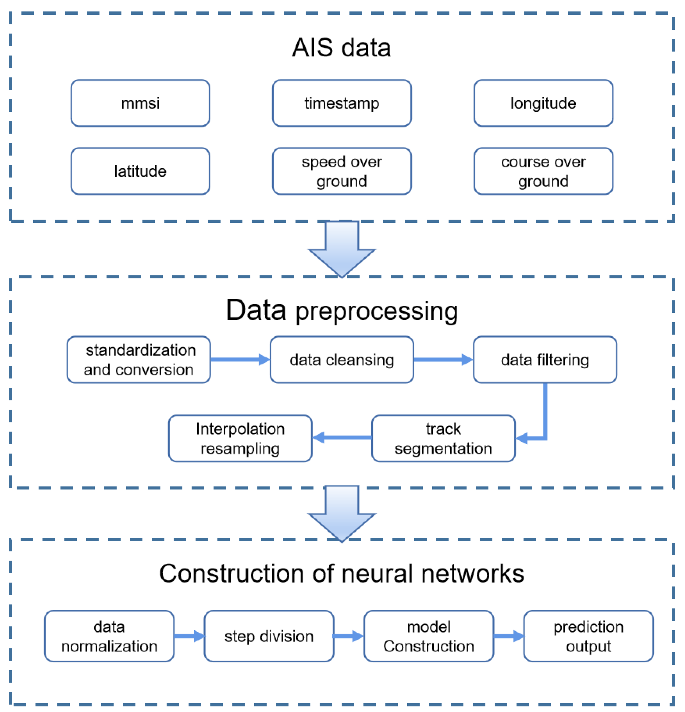
2.1. Data Preprocessing

A ship’s trajectory consists of multiple trajectory points, each containing information {MMSI, TimeStamp, LAT, LON, SOG, COG, VesselType, …, Navigational Status, Draft, Dimension}. In some cases, the ship’s AIS equipment may fail to send complete data or have missing data due to malfunction, signal interference, positional occlusion, etc. In addition, the quality of a ship’s AIS data may be affected by factors such as the performance of the ship’s AIS equipment, the installation location, and the equipment settings, which may lead to inconsistencies in the quality of the data collected. Therefore, data preprocessing is required. Suppose the AIS trajectory of a ship is $T_i=\left\{p_1,p_2,\cdots p_i,\cdots ,p_j\right\}$, where $p_i$ denotes a single trajectory point containing the information {MMSI, TimeStamp, LAT, LON, SOG, COG, VesselType, …, Navigational Status, Draft, Dimension}. Denoting all ship trajectories by $T$, the ship trajectories can then be expressed as $T=\left\{T_1,T_2,\cdots ,T_i\right\}$. The data processing procedure is as follows:

• Data standardization and conversion: In order to reduce data size and improve transmission efficiency, the AIS data are encoded or scaled in some way during transmission and need to be transformed and normalized for subsequent analysis and modeling. For example, the raw data for an automatic identification system are the true latitude and longitude values multiplied by a fixed multiple (usually 600,000), which has the advantage of reducing the data storage space by converting floating-point numbers to integers so that an inverse operation involving dividing by the exact multiple is required to recover the true latitude and longitude values. The timestamps in the AIS raw data are encoded in UNIX timestamps (in seconds from 1 January 1970) and therefore need to be converted to datetime format.
• Data cleansing: inaccurate, incomplete, or invalid data are removed by performing data cleansing. Dealing with missing values, outliers, and duplicates is part of this. Among them, duplicate values or the existence of missing values of a feature in a single trajectory point can be directly deleted for processing. Outliers are detected and processed using thresholds; for example, according to the ITU Radiocommunication Sector M.1371-4 Recommendation points with a heading value greater than 155.2 are deleted, and the points with an SOG > 51.1 are also meaningless because they belong to the noise data and are deleted.
• Data filtering: According to the experimental requirements of this paper, the data features related to trajectory prediction $\left\{t_i,la{t}_i,lo{n}_i,s_i,c_i\right\}$ are denoted TimeStamp, LAT, LON, SOG, and COG. Specific ship types, sailing states, and sailing regions are chosen for filtering to lessen the impact of unimportant factors on the prediction model.
• Track segmentation: Track segmentation is necessary to prevent track drift issues brought on by round trips or other factors. The time interval between successive AIS signals from the same vessel is detected to evaluate whether segmentation is required. When there is a gap of more than six minutes between two pieces of data, segmentation is interrupted, and the track segment with the fewest track points is deleted.
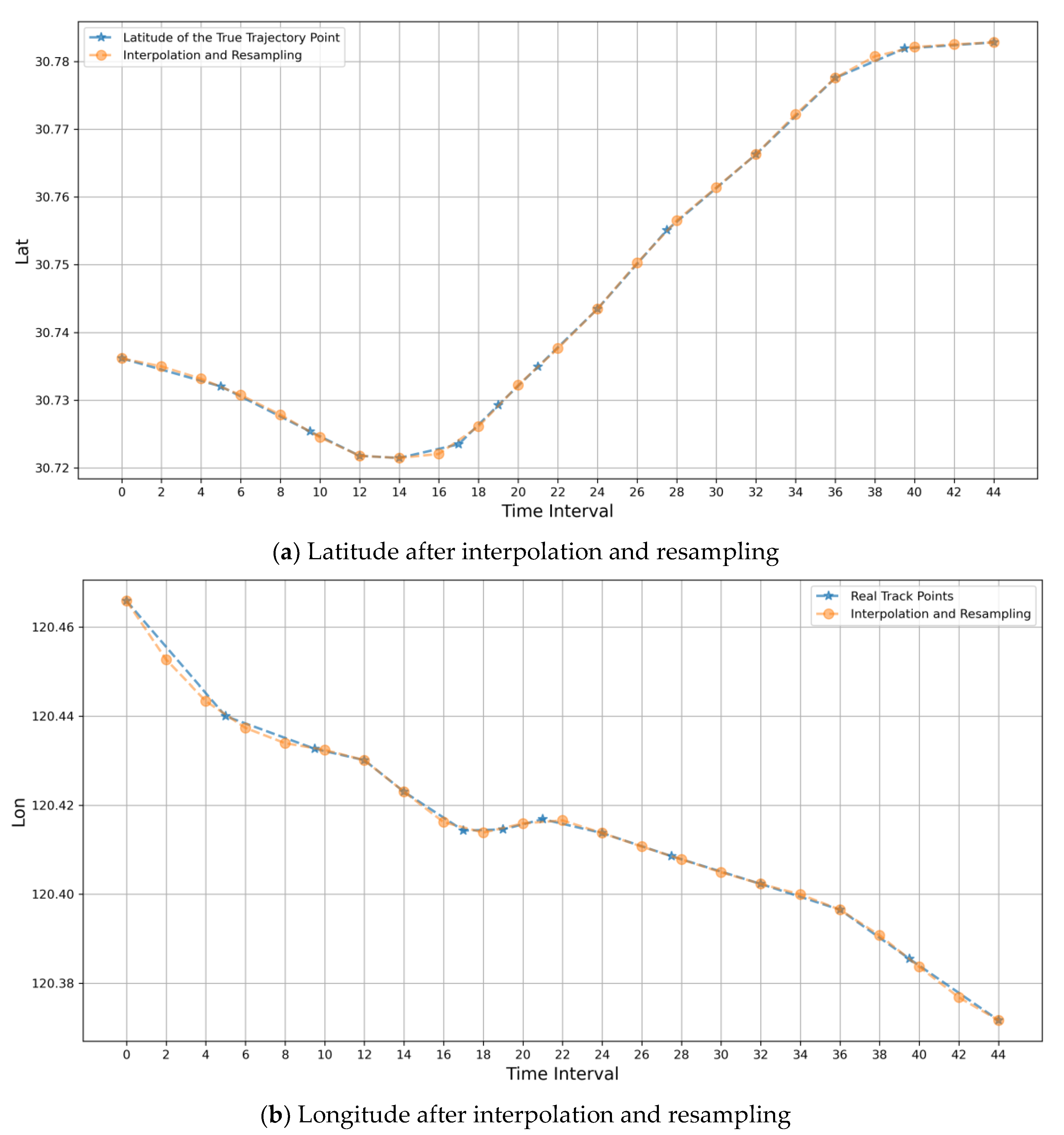
• Interpolation resampling: Because each ship’s AIS data for each trajectory segment are not distributed at equal time intervals, they need to be interpolated. Currently, the most widely used methods are Lagrangian interpolation and spline interpolation. Although Lagrange interpolation passes through all known points as a polynomial function, as the order of the polynomials gets higher and more computationally intensive the interpolation accuracy does not get better and better; on the contrary, the function curve oscillates violently, i.e., the Runge phenomenon. Therefore, to make the function curve able to pass through all the known points and avoid Runge phenomenon, this paper adopts the segmented function; that is, the trajectory points in the trajectory segment are divided into a number of segments; each segment corresponds to an interpolating function. To avoid jittering the curves of functions of too high an order too drastically and creating poor curve fitting with too low an order, cubic spline interpolation is taken to finally obtain an interpolating function sequence, and resampling occurs at two-minute intervals between each track point.

Figure 2 demonstrates the results after cubic spline interpolation and the resampling of latitude and longitude in a trajectory segment; according to the figure, we can observe that this trajectory has a total of 14 trajectory points from 0 to 44 min. The time intervals between neighboring track points are not the same, but the time interval between every two neighboring track points is kept within 6 min. The goal of cubic spline interpolation is to construct a cubic function between every two neighboring trajectory points and to ensure that these cubic functions have continuity at the connection, including 0th-order continuity, first-order derivative continuity, and second-order derivative continuity, so as to achieve the effect of smooth articulation and, ultimately, to obtain a sequence of interpolating functions. And the time is resampled at equal two-minute time intervals; so, the track points are changed from the original 14 to 23, and they generate latitude and longitude 23 accordingly.

2.2. Neural Network Model

2.2.1. LSTM Model

LSTM (long short-term memory) is a recurrent neural network (RNN) variant specifically designed for processing and predicting time series data. Compared with the traditional RNN structure, LSTM introduces a gating mechanism to control the flow of information through gating units, thus effectively solving the problems of traditional RNN in long-term dependency modeling.

The three key gates of the LSTM—the input gate ($i_t$), forget gate ($f_t$), and output gate ($o_t$)—are its central concept. These gates’ functions include controlling information input, forgetting, and output, as well as determining which information should be discarded or retained for the input, state, and output of the current time step. Figure 3 depicts the unit structure of the LSTM, where $c_{t-1}$ denotes the cell state at the previous moment, $h_{t-1}$ denotes the output value at the previous moment, $x_t$ denotes the input at the current moment, $h_t$ denotes the output value at the current moment, $c_t$ denotes the cell state at the current moment, $⨀$ denotes multiplication by elements, $\sigma$ denotes the sigmoid activation function, $w$ is the weight matrix of various gates, and $b$ is the bias term of the corresponding gate.

Specifically, the LSTM works in the following manner:

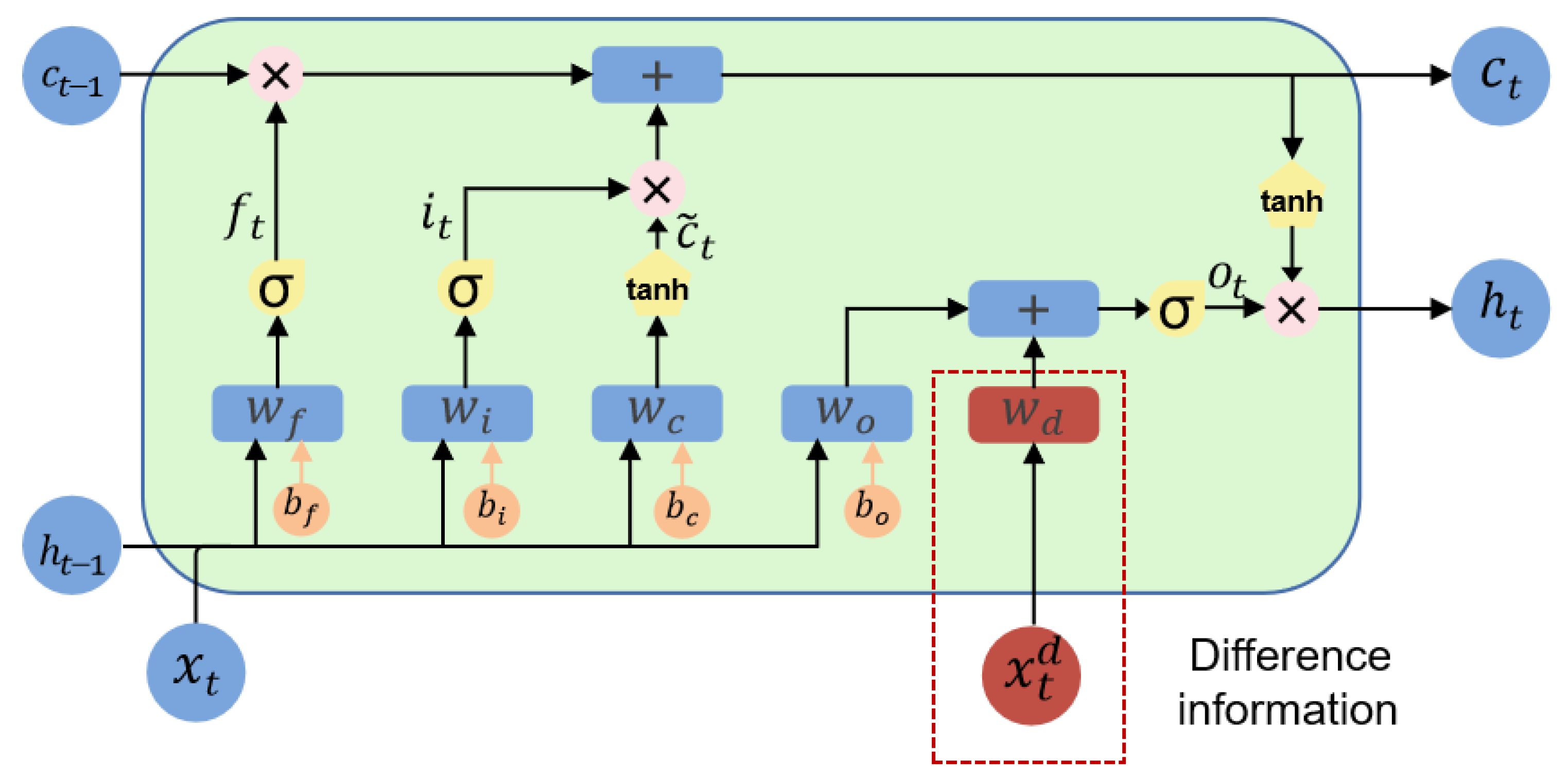
• Input gate: It manages the preservation of input data only in certain areas. It makes a Sigmoid function-based decision regarding how much input data should be incorporated into the cell state for the current time step.

  $$i_t=\sigma (w_i\cdot [h_{t-1},x_t]+b_i)$$

  (1)
• Forget gate: The amount of data from the previous cell state to be forgotten is determined by a sigmoid function. More historical knowledge is lost when the value is closer to 0, whereas more historical knowledge is kept when the value is closer to 1.

  $$f_t=\sigma (w_f\cdot [h_{t-1},x_t]+b_f)$$

  (2)
• Update of the cell state: The tanh activation function processes the output from the previous instant and the input from the current moment to create the input activation vector c. The cell state is then updated by first multiplying the previous moment’s cell state by the forgetting gate by the elements; this is followed by the multiplication of the current input activation vector c by the input gate by the elements.

  $${\tilde{c}}_t=\tanh (w_c\cdot [h_{t-1},x_t]+b_c)$$

  (3)

  $$c_t=c_{t-1}\odot f_t+i_t\odot {\tilde{c}}_t$$

  (4)
• Output gate: This regulates the selective exposure of the output data. The amount of data from the cell state that should be output is determined using a sigmoid function.

  $$o_t=\sigma (w_o\cdot \left[h_{t-1},x_t\right]+b_o)$$

  (5)
• Output: The cell state is processed using the tanh activation function to determine the output of the current time step, which is then multiplied by the output gate’s outcome.

  $$h_t=o_t\odot \tanh (c_t)$$

  (6)

The benefit of an LSTM network is that it can effectively manage long-term dependencies; that is, it can retain information over long periods of time and transmit it when required. In many sequence modeling applications, including speech recognition, natural language processing, and stock price prediction, this enables LSTM to perform effectively.

2.2.2. D-LSTM Model

The difference LSTM (D-LSTM) [24] is an improvement of the traditional LSTM, and the D-LSTM cell is an LSTM cell with difference variables added to the input of the output gate of the LSTM cell, i.e., the difference between the input of the current moment and the input of the previous moment is added. Its model is shown in Figure 4:

The improvement of the D-LSTM over the LSTM lies in the fact that the output gate is calculated as follows:

$$o_t=\sigma (w_o\cdot \left[h_{t-1},x_t\right]+w_d\cdot x_t^d+b_o)$$

(7)

$$x_t^d=x_t-x_{t-1}$$

(8)

where $x_t^d$ is the weight matrix of the difference variable and $w_d$ is the difference variable. D-LSTM emphasizes the use of spatial information more than the regular LSTM does. In order to accurately capture the spatial properties of trajectories, the difference variables used in the trajectory prediction can offer details on the changes in latitude, longitude, speed, and course between trajectory sites. As a result, D-LSTM can predict trajectory more precisely by better integrating temporal and spatial information.

Figure 5 intuitively illustrates the information flow in a three-layer D-LSTM network. Assuming that the dimensions of the original input variables and the difference variables are (1, 4) and that the numbers of neurons in the three layers are 30, 20, and 10, respectively, the total inputs to layer 1 of the D-LSTM are (1, 8). After the information flow through difference layer 1, the output dimension becomes (1, 30); this result is concatenated with the difference information, and its dimension becomes (1, 34). The same is carried out for the third layer. Finally, the output layer is fully connected and contains one unit with output dimension (1).

3. Experimental Results and Analysis

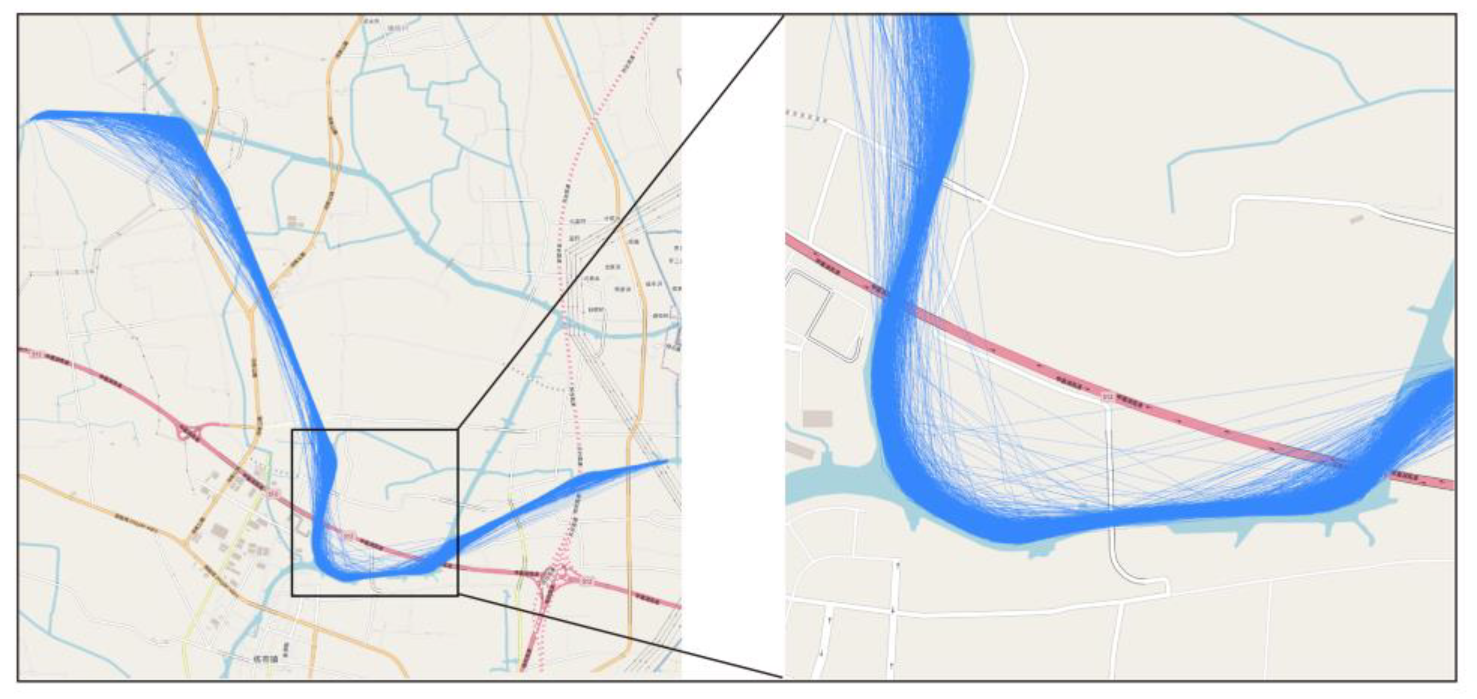
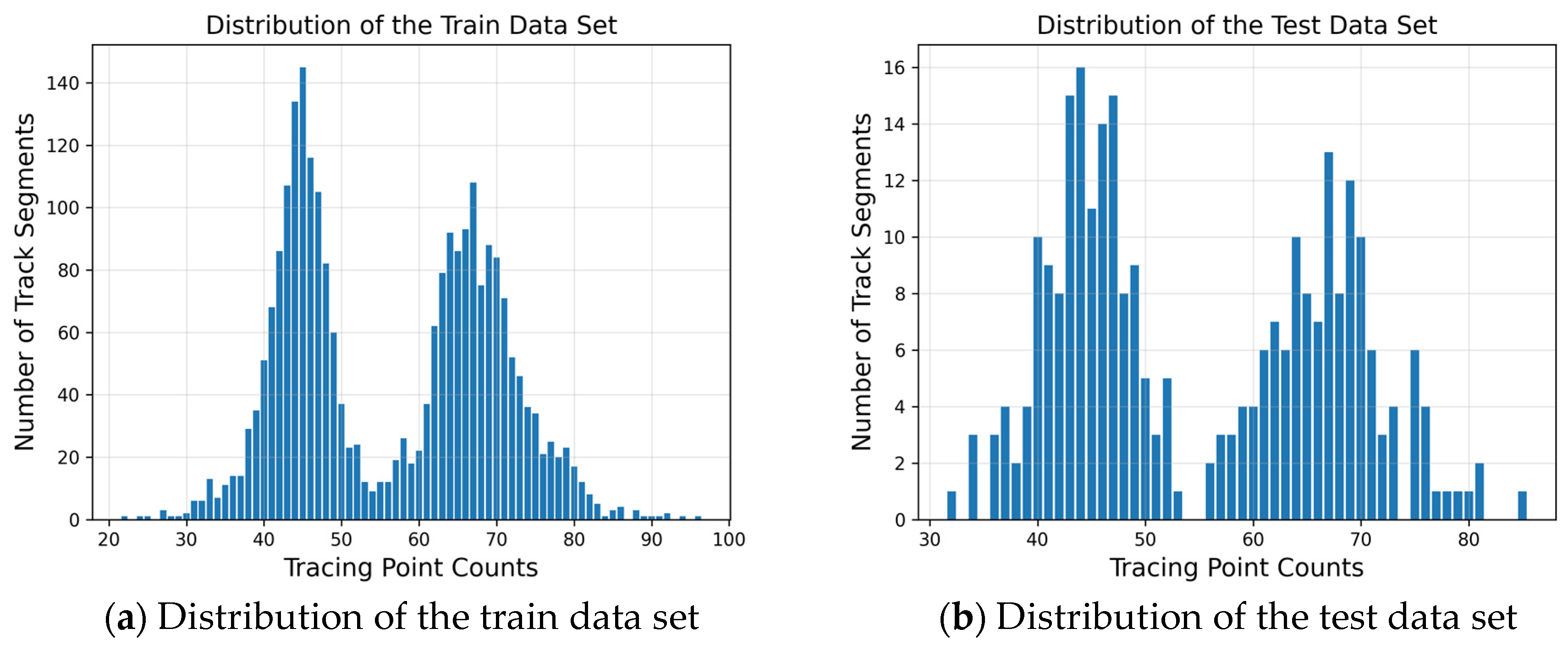
3.1. Data Selection

In this paper, the AIS data of the ships in the Beijing-Hangzhou Canal from September to November 2021 were selected, and the experimental water in the section of Tangjiawan through Beilianli to Nanniwan was selected; it has a wide waterway depth and can accommodate various types of ships and provide better navigational conditions for the ships. However, some curved channel portions in this watershed can affect the navigation efficiency and safety of the ships during the turning process; so, it is crucial to predict and plan the ship voyage. D-LSTM can better capture the spatial attributes of the trajectory points, and it is applicable to both straight and curved channels. It is still difficult for traditional ship prediction algorithms to predict the impact of curved channels. In this paper, D-LSTM was chosen as the research method for trajectory prediction with cargo ships in the region as the research object. Figure 6 shows the ship trajectory map after preprocessing. As can be seen from the figure, there are multiple waterways with large turning angles. The lines appearing on the land at the turn in the figure are there because some ships travel fast and undergo a faster change of position at the turn, resulting in larger intervals between trajectory points of equal time intervals.

The data were normalized to ensure the generality and robustness of the training model and to expedite the model’s training because the range of values for the various aspects of the AIS data varies substantially. In this experimental scenario, the water current greatly impacts the ship’s sailing speed. As a vessel travels downstream in a river, the current provides additional power to the ship, increasing the speed at which the ship moves relative to the ground or seabed. Therefore, when sailing downstream, the ship’s SOG will be relatively high, the sailing time of the same route section will be shorter, and the number of trajectory points after interpolating and resampling them into equal time intervals will be less. Conversely, when sailing against the current, the ship’s SOG will be relatively low, the sailing time in the same section of the route will be longer, and the number of trajectory points after interpolating and resampling them into equal time intervals will be higher. This leads to differences in the number of trajectory points in different segments. As a result, Figure 7 below shows the distribution of the number of trajectory points and trajectory segments in the dataset used for this study. The horizontal axis represents the number of trajectory points, and the vertical axis represents the number of trajectory segments containing that number of trajectory points. There are two peaks in each graph; the first peak has fewer track points because most vessels go downstream and spend less time traveling the same distance, and when the time interval is split, there are fewer track points. The second peak indicates that the ship is sailing against the current, taking longer and having more trajectory points. The training set has 2505 ships, making up 90% of the dataset; there are 141,726 trajectory points. The test set has 279 ships, making up 10% of the dataset; there are 15,386 trajectory points. Each trajectory in the model is given its longitude, latitude, course over ground, and speed over ground as input to a neural network. The neural network performs single-step prediction by using the first ten trajectory points to forecast the eleventh trajectory point.

3.2. Evaluation Metrics

In order to verify the effectiveness of the model, the D-LSTM trajectory prediction model in this study uses three assessment metrics: mean absolute error (MAE), mean square error (MSE), and goodness of fit $R^2$. The higher prediction accuracy of the model is indicated by the decreased values of the MAE and MSE. The model fails to explain the variability of the dependent variable when $R^2$, also known as r equals 0, is present. In other words, the prediction effect of the independent variable on the dependent variable is identical to that of using the mean directly. When $R^2$ is equal to 1, the model fits very well and properly explains the variability of the dependent variable. If $R^2$ is negative, the model fits poorly and its ability to predict outcomes is inferior to that of using the mean directly. The following is the calculation for the three evaluation indicators:

$$MAE=\frac{1}{n}{\displaystyle \sum _{i=1}^n\left|y_i-{\widehat{y}}_i\right|}$$

(9)

$$MSE=\frac{1}{n}{\displaystyle \sum _{i=1}^n{(y_i-{\widehat{y}}_i)}^2}$$

(10)

$$R^2=1-\frac{{\displaystyle {\sum }_{i=1}^n{({\widehat{y}}_i-y_i)}^2}}{{\displaystyle {\sum }_{i=1}^n{(\overline{y}-y_i)}^2}}$$

(11)

where $y_i$ is the true value, ${\widehat{y}}_i$ is the predicted value, $\overline{y}$ is the mean of the true values of the samples in the test set, and $n$ is the number of samples.

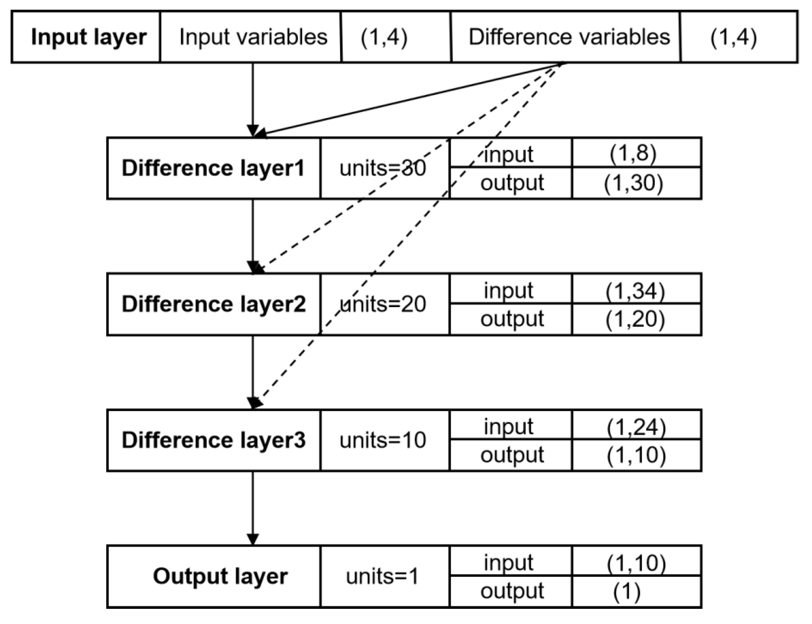
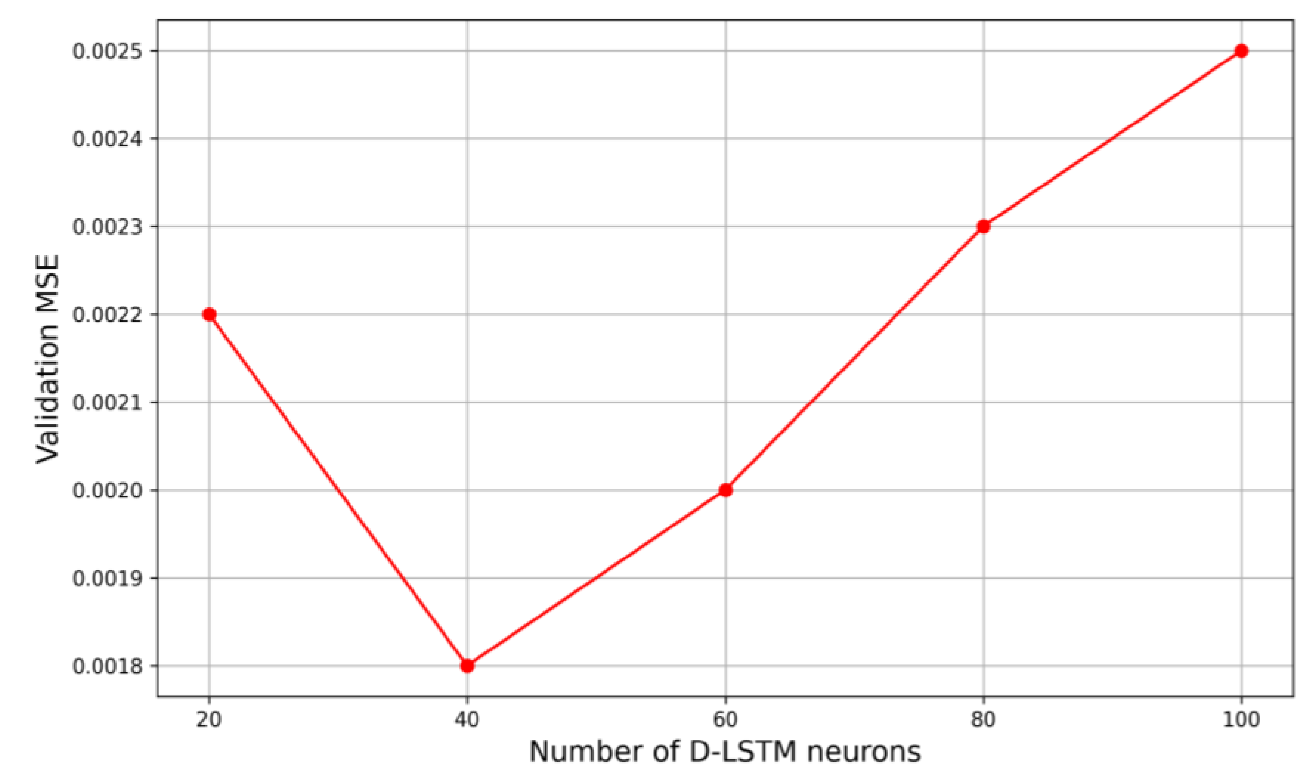
3.3. D-LSTM Architecture and Comparison Models

To construct the optimal D-LSTM model, we compared the D-LSTM model with one, two, and three hidden layers. We found that the prediction of the D-LSTM model with two and three hidden layers was not very good, and the possible reason is that D-LSTM has a more complex structure and is prone to overfitting. Therefore, the D-LSTM model in this experiment consists of a three-layer network divided into an input layer, a D-LSTM layer, and an output layer. We used grid search to train and validate the D-LSTM model from candidate sets 20, 40, 60, 80, and 100 to select the optimal number of hidden units. The validation MSEs for the different neuron numbers are shown in Figure 8. When the neuron number equals 40, the D-LSTM model achieves the best MSE of the validation set.

In this study, we built a D-LSTM neural network model to forecast the ship’s path via the Beijing-Hangzhou Canal from Tangjiawan to Nanniaba via Beilianli. We compared the prediction outcomes with those of the prevalent neural network models currently being utilized in ship trajectory prediction in order to confirm the dependability and accuracy of the created model. Backpropagation (BP), recurrent neural network (RNN), long short-term memory (LSTM), bidirectional long short-term memory (Bi-LSTM), gated recurrent unit (GRU), and bidirectional gated recurrent unit (Bi-GRU) are the six models for the prediction that were chosen.

The detailed parameters of each model are the same, as shown in

Table 1. Neural network training parameters.

validation_split	monitor	loss	optimizer
0.1	val_loss	MSE	Adam
batch_size	learning_rate	factor	min_lr
32	0.01	0.5	0.001

. According to the model’s validation_split = 0.1 setting, 90% of the training dataset is used to learn the parameters and optimize the model. In comparison, the remaining 10% is used as the validation dataset during training to assess the model’s performance and modify its hyperparameters. The loss function of the model is the MSE, which is used to measure the gap between the predicted and true values. The performance of the model is monitored by the loss values on the validation set. Adam was chosen as the optimizer with a batch_size of 32 because it performs well in many deep learning tasks. The learning rate starts out at 0.01 with a lower bound of 0.001 and a learning rate decay factor of 0.5. The learning rate decay approach, the ReduceLROnPlateau callback function, increases the model’s convergence rate and prevents irrational learning rate settings. A learning rate reduction factor is multiplied by the learning rate once the metrics stop improving. The simulation processes were accomplished in a personal computer in Python3.7, with a 64-bit operating system, 8.00 GB of RAM, and Intel(R) Core (T M) i7-6500 [email protected].

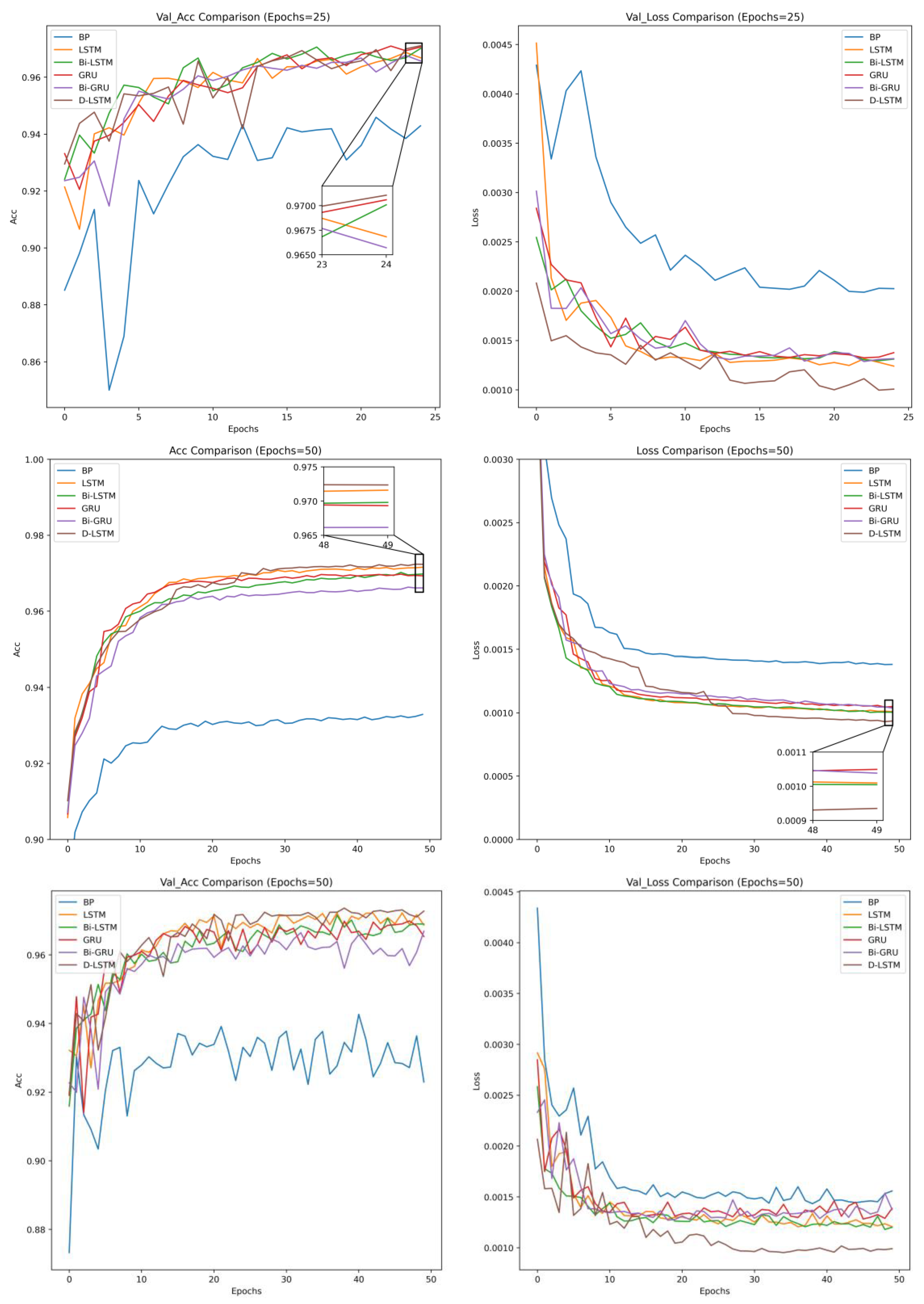
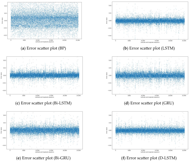
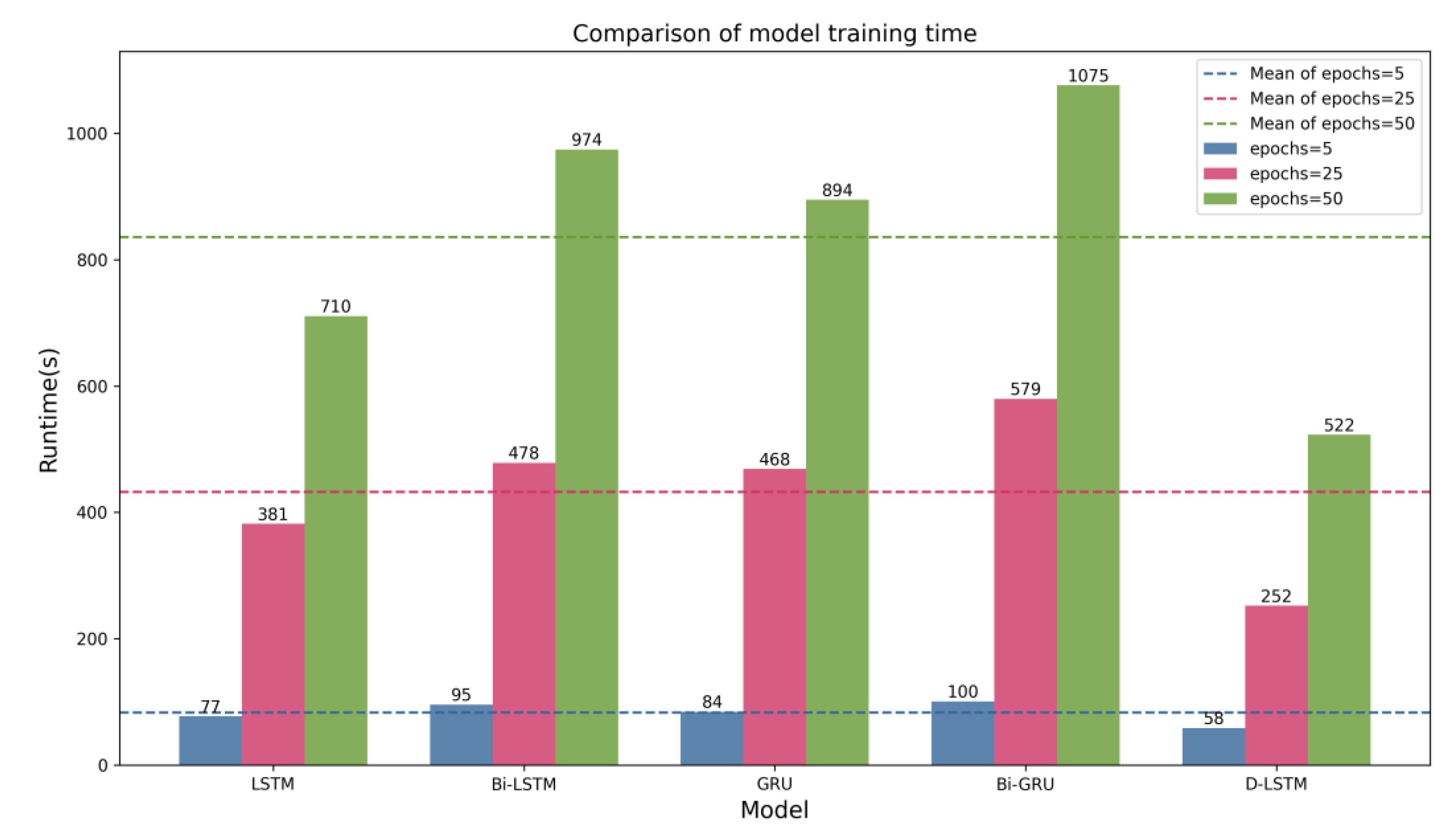
3.4. Analysis of Results

In this paper, the epochs in the model were set to a maximum of 100, and in order to avoid overfitting the model, training was stopped when the validation loss was not decreasing in five consecutive training cycles. It was found that the D-LSTM model had the best fit when epochs = 25. In order to objectively compare the advantages and disadvantages of various models in solving the ship trajectory prediction problem, the prediction performance of each model was compared at the different iterations of 5, 25, and 50. The error metric suggested in 3.2 and the metric of the model training time were used to assess the prediction performance of the models. The neural network’s training parameters are shown in Table 1, where the inputs for the latitude, longitude, heading, and speed of the first 10 trajectory points are used to predict the latitude, longitude, heading, and speed of the eleventh trajectory point. The D-LSTM model has the most minor errors and the best fit compared to other models with smaller errors and better fit, and the model training time of D-LSTM is the lowest. The primary reason may be that the difference variables make the model converge faster; therefore, the training time is lower.

Table 2. Comparison of prediction results and training time of each neural network model.

Model	Epochs	$\mathbf{MAE} (\times {10}^{-2}$)	$\mathbf{MSE} (\times {10}^{-2}$)	${\mathit{R}}^2$	Runtime (s)
BP	5	2.0991	0.2498	0.9604	25.7735
RNN	5	12.5483	6.9686	−0.1043	43.4832
LSTM	5	1.3127	0.1492	0.9764	77.2647
Bi-LSTM	5	1.5549	0.1800	0.9715	95.8038
GRU	5	1.3585	0.1589	0.9748	84.5002
Bi-GRU	5	1.4595	0.1677	0.9734	100.9159
D-LSTM	5	1.2505	0.1435	0.9772	58.8807
BP	25	1.7917	0.2072	0.9672	127.3508
RNN	25	1.4989	0.1667	0.9736	222.0595
LSTM	25	1.0147	0.1232	0.9805	381.7424
Bi-LSTM	25	1.0072	0.1275	0.9798	478.4366
GRU	25	1.0824	0.1352	0.9786	468.6859
Bi-GRU	25	1.0925	0.1303	0.9794	579.7488
D-LSTM	25	0.9982	0.1200	0.9810	252.3140
BP	50	1.7229	0.1533	0.9757	304.3560
RNN	50	34.1576	20.8596	−2.3055	394.6542
LSTM	50	0.9982	0.1243	0.9803	710.7541
Bi-LSTM	50	0.9594	0.1170	0.9815	974.3503
GRU	50	1.0218	0.1338	0.9788	894.6607
Bi-GRU	50	1.0648	0.1362	0.9784	1075.7852
D-LSTM	50	0.9644	0.1203	0.9809	522.9541

lists the prediction performances of each neural network model under different numbers of iterations. It can be seen from the table that the worst fit of RNN is negative when epochs = 5. Each model’s ability to reduce errors and enhance fitting is enhanced when epochs = 25, and the D-LSTM model outperforms the other models in every metric, with epochs = 25 showing the best fit at different numbers of iterations. The D-LSTM model does not have the lowest MAE metric at epochs = 25, most likely because the model oscillates or stagnates as the loss function shrinks, which might be a result of the optimization algorithm’s design. In comparison with other models with high prediction accuracy, the D-LSTM model not only has the most excellent fit and the lowest error, it also has the most pronounced advantage in terms of requiring less training time.

The accuracy and loss values of the training and validation sets are compared in Figure 9 below for each model’s training process with a different number of iterations. Accuracy and loss values are represented as acc and loss for the training set and val_acc and val_loss for the validation set, respectively. Due to its inconsistent performance and significant inaccuracy during the training phase, the RNN model is not shown in the image. According to the figure, each model is still learning with epochs = 5, as seen by the growing trends in acc and val_acc and the lowering trends in loss and val_loss. This suggests that epochs should be increased to continue optimization. The BP model converges slowly, and the accuracy and loss are unacceptable when epochs = 25 or 50, the training and validation sets, respectively. The accuracy and loss of each model level out after 25 iterations; however the D-LSTM model surpasses the others in terms of accuracy and loss values overall.

Figure 10 shows the scatter plot of the latitude and longitude errors of the prediction results of each model when epochs = 25. Because latitude and longitude form a two-dimensional data structure, it is spread into one dimension for the convenience of comparison, and the vertical coordinate of each point indicates the error between the predicted value and the actual observed value; thus, we can observe the distribution of errors between the different models. The closer the vertical coordinate is to 0, the more accurate the prediction results. First, the prediction results of the BP neural network model have too large an error margin, and the distribution of points needs to be more balanced to keep the error within an effective range. This may be due to the limitations of the BP neural network model in handling complex data, resulting in poor prediction performance. Although the LSTM and Bi-LSTM models have smaller errors overall, they still have higher errors than the D-LSTM model, according to the error metrics in Table 2. This may be because the D-LSTM model fuses the difference variables of the dynamic temporal features with the nonlinear features in the serial data; the model effectively utilizes the differential information and enables the error of most of the predicted values to be controlled in the range of −0.002 to 0.002.

The training time for each epoch is calculated and the training times for all the epochs are added to obtain the total training time. Figure 11 below shows that when the training times and mean values of the five models with the most significant predictive performances—LSTM, Bi-LSTM, GRU, Bi-GRU, and D-LSTM—are compared for three different numbers of iterations, it becomes clear that D-LSTM performs the best. The training time of D-LSTM is significantly shorter than that of other models and much smaller than the mean time for all the iterations. Especially at higher iteration numbers, D-LSTM shows a more efficient training speed compared to the other models. Compared to the LSTM, the Bi-LSTM, GRU, and Bi-GRU models, the D-LSTM model’s training time is decreased by 24.7, 38.9, 31.0, and 42.0 percent, respectively, when epochs = 5. When epochs = 25, the D-LSTM model’s training time is reduced by 33.9%, 47.3%, 46.2%, and 56.5%, respectively, when compared to the LSTM, Bi-LSTM, GRU, and Bi-GRU models. When epochs = 50, the training time of the D-LSTM model is less than that of the LSTM, Bi-LSTM, GRU, and Bi-GRU models by 26.5, 46.4, 41.6, and 51.4%, respectively. This demonstrates that D-LSTM offers great optimization capabilities and computational efficiency in ship trajectory prediction models, enabling it to guarantee high-quality prediction performance and drastically shorten training time.

4. Conclusions

By adding differential information between the current moment and the previous moment based on the original data and the previous hidden unit state input, this paper proposes a difference LSTM-based ship trajectory prediction method that addresses the shortcomings of traditional neural network models with low prediction accuracy and long training times. This method captures differences and trends in the sequence data and speeds up model convergence to reduce training time and improve model prediction accuracy. The training procedure and prediction outcomes of the D-LSTM model are then contrasted with those of other deep learning-based ship trajectory prediction models. The findings demonstrate that the proposed method has significantly shorter running times and more accurate ship trajectory predictions. The model’s limitation, however, is that multistep predictions are always subject to low accuracy. This might be because multistep predictions involve predicting a number of future time steps, and the differential operation may cause prediction errors to accumulate at each time step, decreasing accuracy. As a result, the model primarily focuses on short-term changes during the training process. This is interesting for applications in scenarios such as real-time ship navigation, efficient fleet scheduling, ship accident investigation and risk assessment, early warning, and safety management.

References

1. Fan, J. Research on ship positioning navigation and track prediction based on big data technology. Ship Sci. Technol. 2018, 40, 31–33. [Google Scholar]
2. Xu, T.; Cai, F.; Hu, Q.; Yang, C. Research on estimation of AIS vessel trajectory data based on Kalman filter algorithm. Mod. Electron. Tech. 2014, 37, 97–100+104. [Google Scholar] [CrossRef]
3. Jiang, B.; Guan, J.; Zhou, W.; Chen, X. Vessel trajectory prediction algorithm based on polynomial fitting kalman filtering. J. Signal Process. 2019, 35, 741–746. [Google Scholar] [CrossRef]
4. Guo, S.; Liu, C.; Guo, Z.; Feng, Y.; Hong, F.; Huang, H. Trajectory prediction for ocean vessels base on k-order multivariate markov chain. In Wireless Algorithms, Systems, and Applications; Chellappan, S., Cheng, W., Li, W., Eds.; Springer International Publishing: Cham, Vietnam, 2018; pp. 140–150. [Google Scholar] [CrossRef]
5. Rong, H.; Teixeira, A.P.; Guedes Soares, C. Ship trajectory uncertainty prediction based on a gaussian process model. Ocean. Eng. 2019, 182, 499–511. [Google Scholar] [CrossRef]
6. Qiao, S.; Shen, D.; Wang, X.; Han, N.; Zhu, W. A self-adaptive parameter selection trajectory prediction approach via hidden markov models. IEEE Trans. Intell. Transp. Syst. 2015, 16, 284–296. [Google Scholar] [CrossRef]
7. Murray, B.; Perera, L.P. A data-driven approach to vessel trajectory prediction for safe autonomous ship operations. In Proceedings of the Thirteenth International Conference on Digital Information Management (ICDIM), Berlin, Germany, 24–26 September 2018. [Google Scholar] [CrossRef]
8. Wang, J.; Ding, H.; Hu, B. Ship trajectory prediction model based on sliding window PSO-LSSVR. J. Wuhan Univ. Technol. 2022, 44, 35–43+59. [Google Scholar]
9. Mazzarella, F.; Fernandez Arguedas, V.; Vespe, M. Knowledge-based vessel position prediction using historical ais data. In Proceedings of the 2015 Sensor Data Fusion: Trends, Solutions, Applications (SDF), Bonn, Germany, 6–8 October 2015. [Google Scholar] [CrossRef]
10. Qi, L.; Zheng, Z. Trajectory prediction of vessels based on data mining and machine learning. J. Digit. Inf. Manag. 2016, 14, 33–40. [Google Scholar]
11. Jin, X. Analysisand Prediction Method of Vessel Trajectory; Beijing University of Posts and Telecommunications: Beijing, China, 2018. [Google Scholar]
12. Gan, S.; Liang, S.; Li, K.; Deng, J.; Cheng, T. Trajectory length prediction for intelligent traffic signaling: A data-driven approach. IEEE Trans. Intell. Transp. Syst. 2018, 19, 426–435. [Google Scholar] [CrossRef]
13. Hexeberg, S.; Flaten, A.L.; Eriksen, B.-O.H.; Brekke, E.F. AIS-based vessel trajectory prediction. In Proceedings of the 2017 20th International Conference on Information Fusion (Fusion), Xi′an, China, 10–13 July 2017. [Google Scholar] [CrossRef]
14. Lv, G.; Hu, X.; Zhang, Q.; Wei, J. Federated spectral clustering algorithm for ship AIS trajectory AIS. Appl. Res. Comput. 2022, 39, 70–74+89. [Google Scholar] [CrossRef]
15. Xu, T.; Liu, X.; Yang, X. BP neural network-based ship track real-time prediction. J. Dalian Marit. Univ. 2012, 38, 9–11. [Google Scholar] [CrossRef]
16. Quan, B.; Yang, B.; Hu, K.; Guo, C.; Li, Q. Prediction model of ship trajectory based on LSTM. Comput. Sci. 2018, 45 (Suppl. S2), 126–131. [Google Scholar]
17. Hu, Y.; Xia, W.; Hu, X.; Sun, H.; Wang, Y. Vessel trajectory prediction based on recurrent neural network. Syst. Eng. Electron. 2020, 42, 871–877. [Google Scholar]
18. Suo, Y.; Chen, W.; Claramunt, C.; Yang, S. A ship trajectory prediction framework based on a recurrent neural network. Sensors 2020, 20, 5133. [Google Scholar] [CrossRef] [PubMed]
19. Ma, Q.; Zhang, D.; Wang, P.; Liu, Z. Application of bidirectional gated cycle unit in ship trajectory prediction. J. Saf. Environ. 2023, 23, 1–10. [Google Scholar] [CrossRef]
20. Gao, D.; Zhu, Y.; Zhang, J.; He, Y.; Yan, K.; Yan, B. A novel mp-lstm method for ship trajectory prediction based on ais data. Ocean. Eng. 2021, 228, 108956. [Google Scholar] [CrossRef]
21. Liu, R.W.; Liang, M.; Nie, J.; Lim, W.Y.B.; Zhang, Y.; Guizani, M. Deep learning-powered vessel trajectory prediction for improving smart traffic services in maritime internet of things. IEEE Trans. Netw. Sci. Eng. 2022, 9, 3080–3094. [Google Scholar] [CrossRef]
22. Jiang, D.; Shi, G.; Li, N.; Ma, L.; Li, W.; Shi, J. TRFM-ls: Transformer-based deep learning method for vessel trajectory prediction. J. Mar. Sci. Eng. 2023, 11, 880. [Google Scholar] [CrossRef]
23. Altan, D.; Marijan, D.; Kholodna, T. SafeWay: Improving the safety of autonomous waypoint detection in maritime using transformer and interpolation. Marit. Transp. Res. 2023, 4, 100086. [Google Scholar] [CrossRef]
24. Zhou, J.; Wang, X.; Yang, C.; Xiong, W. A novel soft sensor modeling approach based on difference-lstm for complex industrial process. IEEE Trans. Ind. Inform. 2022, 18, 2955–2964. [Google Scholar] [CrossRef]
Figure 1. Ship trajectory prediction flow chart.
Jmse 11 01731 g001
Figure 2. Interpolated latitude and longitude.
Jmse 11 01731 g002
Figure 3. Structure of the LSTM unit.
Jmse 11 01731 g003
Figure 4. Structure of the D-LSTM unit.
Jmse 11 01731 g004
Figure 5. Information flow of a three-layer D-LSTM.
Jmse 11 01731 g005
Figure 6. Vessel trajectory map after preprocessing.
Jmse 11 01731 g006
Figure 7. Training set and test set data distribution.
Jmse 11 01731 g007
Figure 8. Validation MSEs of D-LSTM for different neuron numbers.
Jmse 11 01731 g008
Figure 9. Comparison of accuracy and loss values between the training and validation sets during the training process of each model.
Jmse 11 01731 g009aJmse 11 01731 g009b
Figure 10. Latitude and longitude error scatter plots (epochs = 25).
Jmse 11 01731 g010
Figure 11. Model training time comparison.
Jmse 11 01731 g011