Article

Modulation Effects of Internal-Wave Evolution on Acoustic Modal Intensity Fluctuations in a Shallow-Water Waveguide

1
School of Marine Science and Technology, Northwestern Polytechnical University, Xi’an 710072, China
2
Shaanxi Key Laboratory of Underwater Information Technology, Xi’an 710072, China
3
Qingdao Research Institute, Northwestern Polytechnical University, Qingdao 266200, China
4
Frontiers Science Center for Deep Ocean Multispheres and Earth System and Physical Oceanography Laboratory, Ocean University of China, Qingdao 266100, China
5
Sanya Oceanographic Institution and Key Laboratory of Ocean Observation and Information of Hainan Province, Ocean University of China, Sanya 572024, China
6
Laoshan Laboratory, Qingdao 266237, China
*
Author to whom correspondence should be addressed.
J. Mar. Sci. Eng. 2023, 11(9), 1686; https://doi.org/10.3390/jmse11091686
Submission received: 18 July 2023 / Revised: 18 August 2023 / Accepted: 25 August 2023 / Published: 26 August 2023

Abstract

:
Internal solitary waves evolving with time in shallow water are known to affect sound propagation significantly. Unlike prior work studying the acoustic effects of individual internal-wave properties separately, this paper elucidates and evaluates the influence of a complete evolution process of internal waves on acoustic fields both theoretically and by the coupled ocean-acoustic simulation. Two evolving wave properties considered here are shape deformations including the variations of wave amplitudes and widths and packet dispersion manifested as the increasing wavelength (i.e., the distance between successive solitons). The acoustic modal intensity expressed by the Dyson series solution is reformulated to explicitly reveal the modulation effects induced by the deformation and dispersion of internal waves. Dispersion leads to modal interference and causes the intensity envelope to oscillate with the varying wavelength. Deformation modulates intensity in a non-oscillatory manner that is less predictable due to the complexity of amplitude and width variations. In the environment reconstructed from the field observations of internal waves in the South China Sea, the modal intensity simulated by the parabolic-equation model exhibits pronounced modulation effects, where the modal interference due to dispersion dominates the intensity-envelope shape, and deformation affects the extremum positions of envelopes.

1. Introduction

Acoustic propagation in shallow water is susceptible to internal solitary waves (ISWs) [1] that can induce large perturbations into thermohaline structures and sound speeds [2,3,4]. From generation to dissipation, internal waves usually undergo a complex evolution process [5,6,7], in which shape deformations [8] and packet dispersion [9,10] are known to have substantial impacts on acoustic fields [11,12]. Here, the variations of wave shapes (e.g., amplitudes and characteristic widths) are termed deformations. Since individual solitons within the same packet typically propagate at different speeds [13], the wavelengths of internal waves change with time, which is called dispersion. Following the terminology used in physical oceanography, wavelength is defined as the distance between successive solitons [13].
Up to this point, the relationship between acoustic variability and individual properties of internal waves have been investigated extensively. The pioneer work conducted by Zhou et al. 1991 [11] attributed the observed anomalously large sound transmission loss to the resonant mode coupling that heavily depended on the wavelength of internal waves. Preisig and Duda (1997) [12] approximated a solitary wave by a square wave and explained the dependence of acoustic mode couplings on the width and amplitude of ISWs. Frank et al. 2004 [14] analyzed the sensitivity of the temporal intensity fluctuations of broadband airgun signals to the width and wavelength of ISWs. As a summary and extension of the previous work, Colosi (2008) [15] used the Dyson series solution [16] to the stochastic coupled mode equation [17,18] to derive a theoretical expression of acoustic modal intensity as a function of internal-wave parameters. The effects of amplitude, width, and wavelength on modal intensity were studied separately. Recently, Jiang et al. 2022 [19] considered the influence of irregular bathymetry on the propagation speed of ISWs in the environmental modeling and studied the fluctuations of sound intensity in the continental slope/shelf region. Gao et al. 2023 [20] investigated the acoustic temporal coherence in the presence of nonlinear internal waves and found that the correlation coefficients exhibited quasi-periodicity, the dominant period of which was the same as the periods of ISWs.
However, evolution actually involves the simultaneous changes of various properties of internal waves following physical rules, and the dependence of acoustic variability on the time-varying ISW parameters during a complete evolution process of internal waves remains to be studied. This paper features internal-wave evolution as an integral process rather than the isolated variations of individual wave properties. As a further refinement to the work in Colosi (2008) [15], we reformulate the Dyson-series representation of modal intensity to provide insights into the joint modulation effects of both shape deformation and packet dispersion on sound propagation. The different physical mechanisms by which deformation and dispersion affect the envelope of intensity fluctuations are analyzed, which are further confirmed in the modal intensity simulated by the parabolic-Equation (PE) model in an environment reproduced from an observed ISW packet in the South China Sea (SCS). In turn, the envelope variation of modal intensity obtained from acoustic data can be used to invert the dispersion rate of an ISW train.
The outline of this paper is as follows. In Section 2, we derive the expression of modal intensity as a function of internal-wave parameters using the Dyson series and elucidate the physical mechanisms by which deformation and dispersion modulate the intensity fluctuation. In Section 3, we describe the evolution process of an internal wave event observed in the SCS, and the sound–speed fields perturbed by ISWs are reconstructed for acoustic simulations. In Section 4, the sound fields during internal-wave evolution are calculated by the PE model, and the simulated modal intensity is analyzed to illustrate the modulation effect. In Section 5, we explain the modulation effects of deformation, dispersion, and both of them on modal intensity in the context of the Dyson-series representation obtained in Section 2. Finally, the conclusions of this paper are presented in Section 6.

2. Theoretical Derivation of Modulation Effects in Modal Intensity Fluctuations

2.1. Stochastic Coupled Mode Equation and Its Dyson Series Solution

Following the notations in Dozier and Tappert (1978a) [17] and Colosi (2008) [15], the Dyson-series representation of modal intensity in the single-scattering approximation is first derived in this section. The Helmholtz equation in the cylindrical coordinate system takes the form:
1 r r r p r , z r + ρ ¯ z z 1 ρ ¯ z p r , z z + ω 2 c 2 r , z p r , z = 0 ,
where p ( r , z ) is the complex acoustic pressure, ρ ¯ ( z ) is the background density profile, ω is the acoustic angular frequency, and c ( r , z ) is the sound–speed field. Moreover, p ( r , z ) satisfies (1) the pressure-release boundary condition at the sea surface and (2) the continuity of pressure and vertical particle velocity at the water/bottom interface. Assuming that internal waves cause sound–speed perturbations δ c ( r , z ) to the background profile c ¯ ( z ) , the range-dependent c ( r , z ) is given by:
c r , z = c ¯ z + δ c r , z .
The pressure p ( r , z ) in Equation (1) can be written in terms of normal modes, that is:
p r , z = n = 1 N a n r k n r ϕ n z ,
where a n ( r ) and k n are the range-dependent modal coefficient and the real part of the horizontal wavenumber of the nth mode, respectively, N is the number of acoustic modes, and ϕ n ( z ) is the modal function in the background environment. Then, the rapidly oscillating phasor exp ( i l n r ) is removed from a n ( r ) to get the demodulated modal coefficient a ˜ n ( r ) , i.e., the complex envelope of a n ( r ) :
a ˜ n r = a n r exp i l n r ,
where l n = k n + i α n is the horizontal wavenumber of mode n and the imagery part α n accounting for sound attenuation can be estimated by the perturbation theory [21]. The range evolution of a ˜ n ( r ) is governed by the stochastic coupled mode equation [17,18]:
d a ˜ n r d r = i m = 1 N R n , m r exp i l m , n r a ˜ m r , l m , n = l m l n ,
where
R n , m r = k 0 2 k n k m 0 δ c r , z c 0 ϕ n z ϕ m z ρ ¯ z d z
is the coupling matrix, c 0 is the reference sound speed, and k 0 = ω / c 0 is the reference wavenumber.
Equation (5) does not have an exact analytical solution. We now approximate a ˜ n ( r ) by the Dyson series [16] and expand a ˜ n ( r ) at a receiver range r = r RX to the first order, yielding:
a ˜ n r RX = a ˜ n 0 + i m = 1 N S n , m 1 a ˜ m 0 ,
where a ˜ n ( 0 ) is the modal coefficient at the source range r = 0 , and S n , m ( 1 ) is the first-order scattering matrix:
S n , m 1 = d k R n , m k 0 r RX d r exp i l m , n k r .
where R n , m ( k ) in the scattering matrix is the Fourier transform of R n , m ( r ) . The modal intensity | a n ( r RX ) | 2 is defined as the squared modulus of the modal coefficient a n ( r RX ) [22]. Combining Equations (4) and (7) and keeping | a n ( r RX ) | 2 to the first order, the modal intensity in the Dyson-series form is written as:
a n r RX 2 = a n 0 2 + 2 m = 1 N a n 0 a m 0 Im S n , m 1 exp 2 α n r RX .
To obtain an analytical form of Equation (9), Colosi (2008) [15] used the Gaussian wave packet as the waveform of ISWs:
A r ; t = j = 1 J η t ; j exp r r p t ; j Δ t ; j 2 ,
where J is the total number of individual solitons within the packet and η ( t ; j ) , r p ( t ; j ) , and Δ ( t ; j ) denote the wave amplitude, peak position, and characteristic width of soliton j varying with time t, respectively. The sound–speed perturbation δ c ( r , z , t ) caused by internal waves is expressed as:
δ c r , z ; t = c 0 d c d z ptnl W 1 z A r ; t ,
where ( d c / d z ) ptnl is the potential sound–speed gradient [15,23] and W 1 ( z ) is the first-order internal-wave modal functionsatisfying the Taylor–Goldstein equation and the rigid-lid boundary condition [24]. Under the condition that the receiver range is large ( r RX ), and that the modal attenuation is small ( α n , α m 0 ), substituting Equation (11) into Equation (9) with some manipulations yields the analytical form of modal intensity, that is:
a n r RX ; t 2 = a n 0 2 + m = 1 N j = 1 J F n , m t ; j sin k m , n r p t ; j ×   exp 2 α n r RX , k m , n = k m k n ,
where
F n , m t ; j = 2 π a n 0 a m 0 Q n , m t ; j Δ t ; j exp k m , n 2 Δ 2 t ; j 4 ,
and
Q n , m t ; j = η t ; j c 0 k 0 2 k n k m 0 d c d z ptnl W 1 z ϕ n z ϕ m z ρ ¯ z d z .

2.2. Modulation of Evolving ISWs on Modal Intensity Fluctuations

For clarity, the contribution from an arbitrary single incident mode m in Equation (12) is taken to discuss the influence of internal-wave evolution. The interference between the received mode n and the incident mode m is described by:
G n , m t = j = 1 J G n , m t ; j = j = 1 J F n , m t ; j sin k m , n r p t ; j ,
and is further expanded in the ascending order as to the soliton numbering j:
G n , m t = F n , m t ; 1 sin k m , n r p t ; 1 + F n , m t ; 2 sin k m , n r p t ; 2 +   F n , m t ; 3 sin k m , n r p t ; 3 + + F n , m t ; J sin k m , n r p t ; J .
Equation (16) provides information about the dependence of the mode-coupling strength on the wavelength of internal waves. That is, the fluctuation magnitude of G n , m ( t ) reaches to the maximum when the distance between successive solitons is equal to an integer multiple of the interference length L n , m determined by modes n and m, that is:
r p t ; j r p t ; j + 1 = L n , m = 2 q π k m , n , q = 1 , 2 , ,
which is called the resonant mode coupling [3,11,15].
However, the influence of packet dispersion on G n , m ( t ) remains implicit in Equation (16) and is not integrated with the effect of shape deformation reflected in F n , m ( t ; j ) . The modulation effects of deformation and dispersion on modal intensity can be made explicit by the following mathematical manipulations. Using trigonometric identities, the superposition of any two successive terms (e.g., j and j + 1 ) in Equation (16) can be written as:
G n , m t ; j , j + 1 = F n , m t ; j sin k m , n r p t ; j + F n , m t ; j + 1 sin k m , n r p t ; j + 1 = 2 F n , m t ; j cos k m , n Λ p t ; j , j + 1 2 sin k m , n r c t ; j , j + 1 Polychromatic term : p o l y n , m t ; j , j + 1 +   F n , m t ; j + 1 F n , m t ; j sin k m , n r p t ; j + 1 Monochromatic term : m o n o n , m t ; j , j + 1 ,
where
r c t ; j , j + 1 = r p t ; j + r p t ; j + 1 2
is the position of the geometric center (also called the centroid) of the “dual-wave packet” composed of the two successive solitons j and j + 1 , and
Λ p t ; j , j + 1 = r p t ; j r p t ; j + 1
is the distance between solitons, i.e., the wavelength of the dual-wave packet.
As formulated in Equation (18), G n , m ( t ; j , j + 1 ) is decomposed into the superposition of the polychromatic term:
p o l y n , m t ; j , j + 1 = 2 F n , m t ; j Deformation-dependent amplitude cos k m , n Λ p t ; j , j + 1 2 Dispersion-dependent interference Polychromatic envelope ×   sin k m , n r c t ; j , j + 1 Carrier wave
and the monochromatic term:
m o n o n , m t ; j , j + 1 = F n , m t ; j + 1 F n , m t ; j Monochromatic envelope sin k m , n r p t ; j + 1 Carrier wave .
Equation (21) shows that p o l y n , m ( t ; j , j + 1 ) can be thought of as a high-frequency carrier wave with amplitude modulation. Typically, the centroid moves at speed d r c / d t of order 1   m / s , whereas the dispersion rate of a dual-wave train is d Λ p ( t ) / d t of much smaller order 0.1   m / s . Therefore, the movement of the centroid is responsible for the rapidly varying modal interference indicated by sin ( k m , n r c ( t ) ) in Equation (21).
Regarding the polychromatic envelope, there are two factors modulating the carrier wave together: one is dependent on packet dispersion; the other is associated with shape deformations. As the dual-wave packet disperses with time, the increasing Λ p ( t ) gives rise to the interference between modes n and m. Thus, the carrier wave is modulated in the form of harmonic oscillation indicated by cos ( k m , n Λ p ( t ) / 2 ) in Equation (21). In contrast to the dispersion typically manifested as the increase in wavelength, the variations of amplitude and width are heavily dependent on the environmental factors (e.g., stratification, topography, etc) of a specific sea area. Consequently, the modulation effect due to deformation may not be as regular as that caused by dispersion and is less predictable.
The composition of m o n o n , m ( t ; j , j + 1 ) in Equation (22) is simpler than that of p o l y n , m ( t ; j , j + 1 ) . It is clear that only the movement of soliton j + 1 (i.e., the last wave in the dual-wave packet) leads to the modal interference at a single frequency, and that only deformation contributes to the amplitude modulation.
Applying the manipulation described by Equation (18) to Equation (16), we obtain another form of G n , m ( t ) :
G n , m t = p o l y n , m t + m o n o n , m t ,
where p o l y n , m ( t ) is the polychromatic component:
p o l y n , m t = J = 1 J 1 1 J 2 j = 1 J 1 j F n , m t ; j Deformation-dependent amplitude   cos k m , n Λ p t ; J , J + 1 2 Dispersion-dependent interference Polychromatic envelope ×   sin k m , n r c t ; J , J + 1 Carrier wave ,
and m o n o n , m ( t ) is the monochromatic component:
m o n o n , m t = 1 J j = 1 J 1 j F n , m t ; j Monochromatic envelope   sin k m , n r p t ; J Carrier wave .
By comparing Equation (16) with Equations (23)–(25), it is found that the use of trigonometric identities transforms G n , m ( t ) from the superposition form (see Equation (16)) into a form containing the product representation (see Equation (24)), thus accentuating the effect of dual-wave packets rather than individual solitons on acoustic intensity. Based on the above derivation, we next focus on the evolution process of a typical internal wave event observed in the SCS and investigate how shape deformations and packet dispersion modulate the acoustic intensity fluctuations in reality.

3. Sea-Trial Observation and Sound–Speed Reconstruction

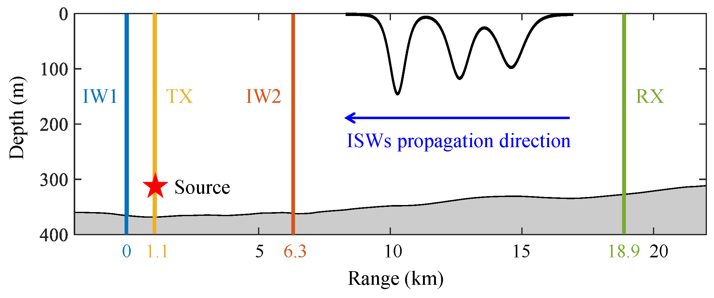
3.1. Experiment Description

The 2019 joint oceanographic-acoustic observation experiment was conducted on the continental shelf in the SCS. The mooring positions and the topography along the track are shown in Figure 1, and the bathymetry data used in this paper are from the GEBCO database [25]. There were a total of four moorings deployed along the track, and two of them were oceanographic moorings IW1 and IW2 equipped with temperature-pressure (TP) sensors, which were deployed 6.3 km apart. One was an acoustic mooring TX positioned 1.1 km away from IW1, on which a transducer was installed at 330.5-m depth and emitted five cycles of linear frequency-modulated (LFM) pulses sweeping from 400 to 500 Hz with a 10-s duration and a 20-s period every hour. The last one was a hybrid mooring RX equipped with both hydrophones and TP sensors and was deployed 18.9 km away from IW1.
The water depth decreased from 365 m (IW1) to 327 m (RX) with a mean value of 349 m and a mild slope of 0.1°. Internal waves propagated from RX to IW1, and sound transmission was in the opposite direction.

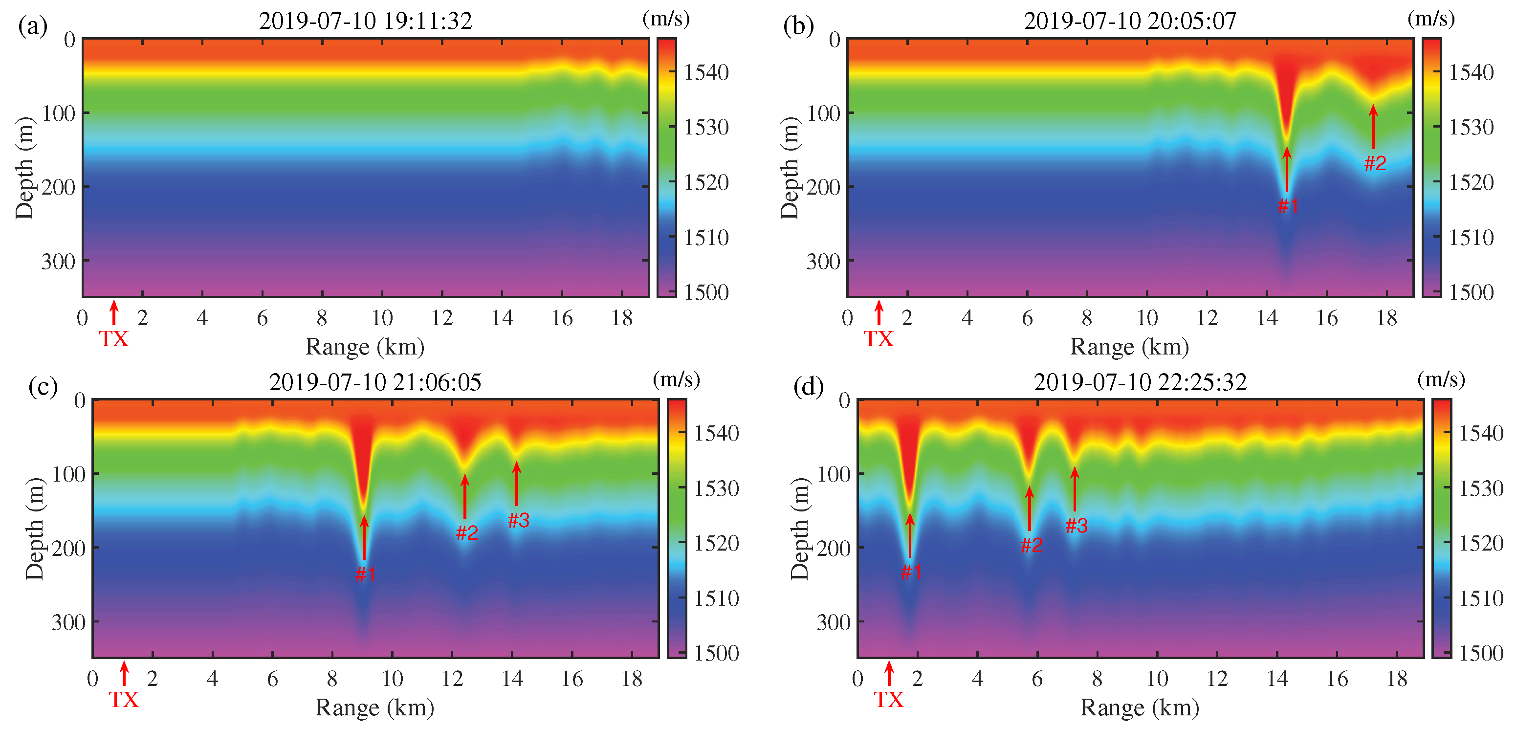
3.2. Oceanographic Observation

A total of 25 groups of internal waves were captured in the experiment, among which the fourth internal wave event (hereafter called Event 4) underwent a typical evolution process and is chosen for analysis in this paper. The temperature profiles measured at IW1, IW2, and RX during Event 4 are shown in Figure 2a–c, respectively, along with the 22.5   ° C isotherms denoted by blue lines. The individual solitons identified from data are annotated by red arrows. The in situ sound–speed profiles (SSPs) at IW1, IW2, and RX are displayed in Figure 2d–f, correspondingly.
The comparison of observations at IW1, IW2, and RX reveals that the internal waves exhibited shape deformations and packet dispersion as they propagated. The deformations were manifested as (1) the variations of wave amplitudes among moorings evidenced by the isothermal displacements and (2) the decreasing width of soliton #2. The dispersion can be seen from the increase in arrival time difference between solitons #1 and #2.

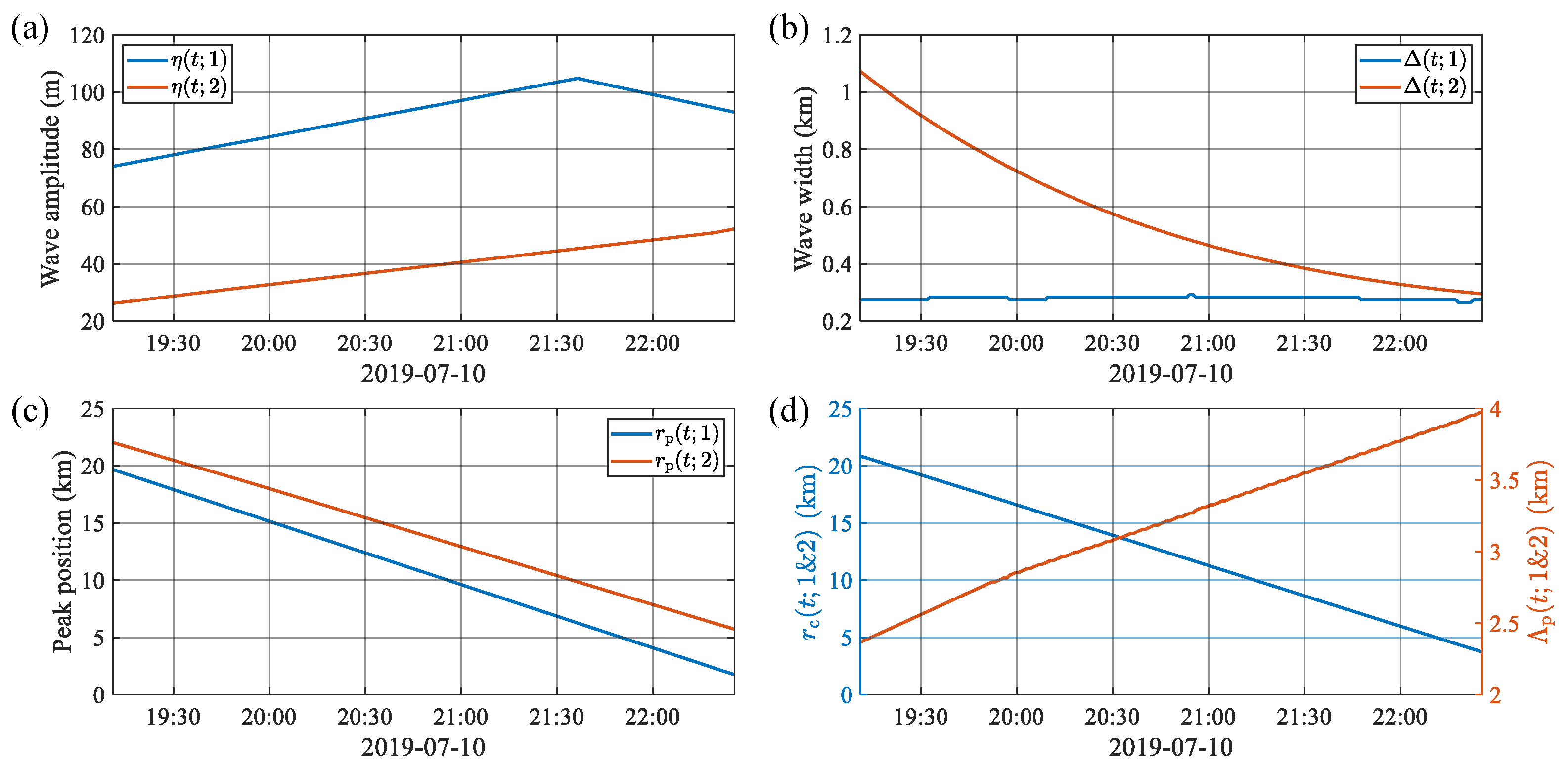
3.3. Reconstruction of Sound–Speed Fields

Before studying the sound propagation through internal-wave fields, we need to reconstruct the acoustic environment with high resolution in horizontal range and full coverage in vertical depth. Note that the time-independence of the modal coefficient a n ( 0 ) at range r = 0 in Equation (12) makes this Dyson-series representation only applicable to the case where the environment at the source position is time-invariant. In view of this, we are concerned with the propagation of internal waves between 19:11 and 22:25, during which the leading edge of the wave packet has not reached mooring IW1 so that the SSP at the source position can be assumed not to change with time.
The dispersive evolutionary propagated thermistor string (DEPTS) method [26] is applied to reconstruct the sound speeds perturbed by Event 4. The modeled sound–speed fields at 19:11:00, 20:05:07, 21:06:05, and 22:25:32 are depicted in Figure 3a–d as examples, respectively, where the individual solitons and the acoustic source position are denoted by red arrows. The topography in calculations is assumed to be flat with a water depth of H = 349   m . These reproduced sound–speed fields will be used as input parameters to the acoustic simulation performed in the next section.

4. PE Simulation and Phenomenon Analysis of Modulation Effects

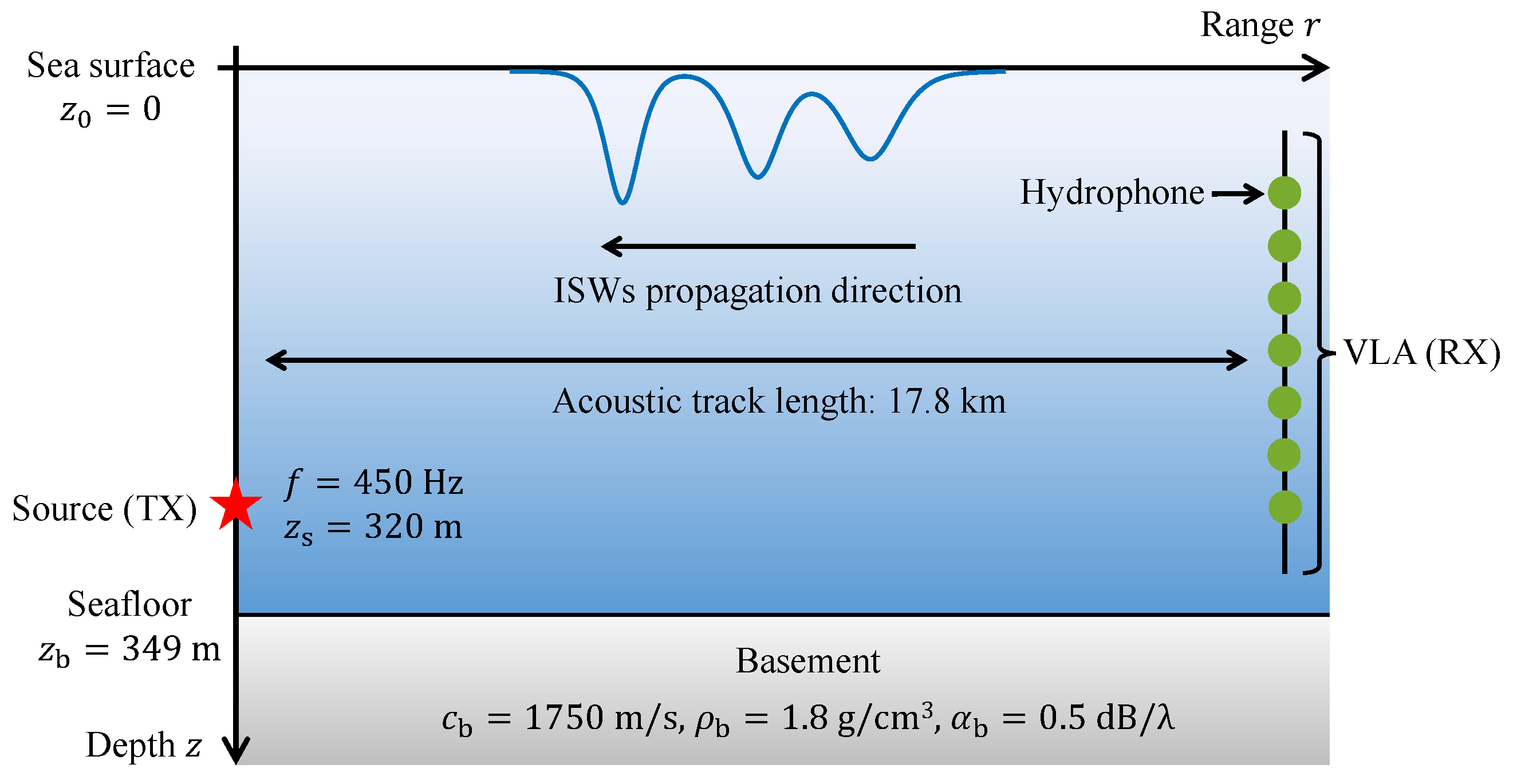
4.1. Configuration and Method

The schematic of the waveguide model used in this paper is depicted in Figure 4 with simulation parameters and is in general agreement with the experimental environment. The continuous-wave (CW) signals at 450 Hz are emitted by a source near the seafloor of depth z b = 349   m and are received by a vertical line array (VLA) equipped with hydrophones at a distance of 17.8 km. Since a flat bottom is adopted in the simulation, the modeled source depth is scaled from the actual value z s , obs = 330.5   m to z s = z s , obs z b / z b , obs 320   m , where z b , obs = 360.5   m is the actual water depth at mooring TX. The bottom is modeled as a homogeneous halfspace with sound speed c b = 1750   m / s , density ρ b = 1.8   g / c m 3 , and attenuation rate α b = 0.5   d B / λ [27], where λ denotes the acoustic wavelength.
With the sound speeds modeled by DEPTS being input parameters, acoustic fields p ( r , z ; t ) are calculated by the computer code IFD [28] based on the PE model. Next, using the orthonormality relation of normal modes [23], mode decomposition is applied to the pressure p ( r RX , z ; t ) received by the VLA at range r = r RX to obtain the modal intensity:
a n r RX ; t PE 2 = k n r RX 0 p r RX , z ; t ϕ n z ρ ¯ z d z 2 ,
where modal functions ϕ n ( z ) are calculated by the KRAKEN program [29].

4.2. Simulation Results and Analysis

A case study of the modulation effect in the first-order modal intensity | a 1 ( r RX ; t ) | PE 2 is carried out in this section. Figure 5a shows the | a 1 ( r RX ; t ) | PE 2 (blue) as a function of time (the bottom x-axis) and of the centroid position (the top x-axis). Here, the geometric center of the dual-wave packet composed of solitons #1 and #2 is designated as the centroid since these two solitons are the most prominent in the wave train, and the following solitons are not well-developed until 22:25:32 as shown in Figure 3d. The upper and lower envelopes are denoted by red-dashed lines. The peak-to-peak values (PPVs) defined as the difference between the upper and lower envelopes are used to quantify the fluctuation magnitude and are displayed by the green line on the right y-axis. It can be seen that | a 1 ( r RX ; t ) | PE 2 exhibits quasi-periodicity with a dominant period of about 30 min. The high-frequency oscillation is modulated by a slowly varying process as evidenced by the envelopes. The PPVs suggest that the fluctuation magnitude increases since internal waves enter the track at 19:11 and reaches its maximum at 20:25, after which it starts to decrease.
With regard to the range scale on the top x-axis in Figure 5a, it was found that after | a 1 ( r RX ; t ) | PE 2 oscillates at the dominant frequency for one cycle, the centroid moves about 2.65 km, close to the interference length L 1 , 2 = 2 π / | k 1 k 2 | = 2.84   km determined by the received mode n = 1 and the incident mode m = 2 . The wavenumber spectrum of | a 1 ( r RX ; t ) | PE 2 is shown in Figure 5b with three pronounced peaks. The first spectral peak appears at k = 2.21 × 10 2   rad / m , close to the horizontal wavenumber difference k 1 , 2 = k 1 k 2 , and thus, represents the interference between modes n = 1 and m = 2 , which is annotated by “Modes 1 & 2 ” in Figure 5b. Similarly, the other two peaks corresponding to the interference between modes 1 & 3 and between modes 1 & 4 are also identified, and it is clear that the first peak is at least 7 dB higher than others.
The above analyses in both the range and wavenumber domains demonstrate that the interference between modes 1 and 2 contributes most to the intensity fluctuation, and thus, the modulation effect found in the time domain. The formation mechanism of the highly variable fluctuation magnitude shown in Figure 5a will be investigated in the next section.

5. Mechanism Study of Modulation Effects Caused by Deformation and Dispersion

5.1. Study Approach

The following simplifications are made here to facilitate the theoretical interpretation of the modulation effect found in Figure 5. Since the interference between modes 1 and 2 dominates the intensity fluctuation, the Dyson-series representation in Equation (12) only including G 1 , 2 ( t ) is calculated to explain the physical mechanism behind the modulation effect in the above PE-simulation results. Besides, the entire ISW train observed in the experiment is approximated by a Gaussian wave packet consisting of the two most prominent leading waves (i.e., solitons #1 and #2 in Figure 3).
We now express the modal intensity | a 1 ( r RX ) | 2 in the partial-Dyson series form:
a 1 r RX ; t Dyson : 2 2 = a 1 0 2 + G 1 , 2 t exp 2 α 1 r RX = a 1 0 2 + j = 1 2 G 1 , 2 t ; j exp 2 α 1 r RX ,
where only the contribution from the incident mode 2 is included in the series. Referring to Equations (23)–(25), G 1 , 2 ( t ) in Equation (27) is rewritten as:
G 1 , 2 t = p o l y 1 , 2 t + m o n o 1 , 2 t ,
where
p o l y 1 , 2 t = 2 F 1 , 2 t ; 1 Deformation-dependent amplitude cos k m , n Λ p t ; 1 , 2 2 Dispersion-dependent interference Polychromatic envelope ×   sin k 2 , 1 r c t ; 1 , 2 Carrier wave
is the polychromatic component, and
m o n o 1 , 2 t = F 1 , 2 t ; 2 F 1 , 2 t ; 1 Monochromatic envelope sin k 2 , 1 r p t ; 2 Carrier wave
is the monochromatic component.
The wave parameters of Event 4 are output from the DEPTS model [26] and are used to calculate the Dyson-series representation given by Equation (27). The wave amplitudes η ( t ; j ) , characteristic widths Δ ( t ; j ) , and crest positions r p ( t ; j ) of solitons j = 1 , 2 are presented in Figure 6a–c, respectively. The centroid position r c ( t ; 1 , 2 ) and the wavelength Λ p ( t ; 1 , 2 ) are shown in Figure 6d. It is clear that as the wave packet propagates along the track, η ( t ; 2 ) keeps increasing while η ( t ; 1 ) starts to decrease after reaching its maximum at 21:36; Δ ( t ; 2 ) keeps decreasing while Δ ( t ; 1 ) are much more stable; soliton #1 moves faster than soliton #2, and hence, Λ p ( t ; 1 , 2 ) keeps increasing. In addition, Figure 7a,b illustrate the potential sound–speed gradient ( d c / d z ) ptnl and the first-order modal function W 1 ( z ) of internal waves, respectively, used to calculate the sound–speed perturbation δ c ( r , z ; t ) given by Equation (11).
Next, we first analyze the influence of deformation and dispersion separately and then discuss the joint modulation effect of these two factors on modal intensity from the perspective of a complete ISW evolution process observed in reality.

5.2. Modulation Effect Induced by Deformation

To study the influence of deformation exclusively, packet dispersion is neglected in this section by setting Λ p ( t ; 1 , 2 ) to remain constant after 20:05 when soliton #2 has entered the track. The modal intensities calculated by the PE model ( | a 1 ( r RX ; t ) | PE 2 ) and by the partial Dyson series ( | a 1 ( r RX ; t ) | Dyson : 2 2 ) are shown in Figure 8a by the blue and red lines, respectively. The PPVs of | a 1 ( r RX ; t ) | PE 2 and | a 1 ( r RX ; t ) | Dyson : 2 2 are given in Figure 8b with the same color scheme. It can be seen from Figure 8a that the two solutions have similar dominant frequencies, whereas the temporal variations of envelopes are different. Figure 8b shows that the relative change in the PPV of the Dyson series solution after 20:05 is only 0.12 / 0.1 = 1.2 , obviously smaller than that of the PE result ( 0.115 / 0.03 3.8 ). Consequently, the fluctuation magnitude of | a 1 ( r RX ; t ) | Dyson : 2 2 is less variable than that of | a 1 ( r RX ; t ) | PE 2 , and the modulation effect caused only by deformation is less pronounced.
To explain the above observations, the interactions among the individual terms annotated in Equations (29) and (30) are examined in more details. Figure 9a,c depict the envelope (purple-solid) and carrier wave (green) of p o l y 1 , 2 ( t ) , respectively, where the deformation-dependent amplitude 2 F 1 , 2 ( t ; 1 ) (purple-dashed) and the dispersion-dependent interference cos ( k 2 , 1 Λ p ( t ) / 2 ) (orange) are also given. The envelope and carrier of m o n o 1 , 2 ( t ) are shown in Figure 9b,d, respectively. The superposition of p o l y 1 , 2 ( t ) (blue) and m o n o 1 , 2 ( t ) (yellow) and the resulting G 1 , 2 ( t ) (red) are illustrated in Figure 9e.
The comparison between Figure 9a,b indicates that the magnitude of the monochromatic envelop is smaller than that of the polychromatic one. Therefore, the modulation effect in G 1 , 2 ( t ) is mainly determined by the polychromatic envelope, as shown in Figure 9e. It is clear from Figure 9a that since Λ p ( t ) no longer changes with time after 20:05, cos ( k 2 , 1 Λ p ( t ) / 2 ) stops oscillating and remains constant. Next, deformation starts to solely determine the polychromatic envelope that drops to its minimum at 21:40 and then increases with only a minor variation. Consequently, the modulation effect in | a 1 ( r RX ; t ) | Dyson : 2 2 governed by the polychromatic envelope is different from that in | a 1 ( r RX ; t ) | PE 2 .
The above discussion reveals that the modulation effect induced by deformation only is not pronounced as compared to the PE result. Referring to Equation (13), the coupling between modes n and m is significant when the wave width satisfies the following condition [15]:
Δ t ; j = L n , m 2 π .
However, in reality, the significance and manifestation of the modulation effect induced by shape deformations are less predictable. This is because remarkable discrepancies may occur in the variations of widths for different solitons in the packet. The condition given by Equation (31) is hard to hold for all solitons simultaneously. Additionally, as formulated in Equations (13) and (14), the variations of wave amplitudes η ( t ; j ) during a long-term evolution process also introduce uncertainties into the modulation effect. Specific to our case here, Figure 10 shows the oscillation amplitudes F 1 , 2 ( t ; j ) of the interference components G 1 , 2 ( t ; j ) for solitons j = 1 , 2 . By comparing Figure 6a,b with Figure 10, it can be seen that η ( t ; 1 ) dominates F 1 , 2 ( t ; 1 ) more than Δ ( t ; 1 ) because Δ ( t ; 1 ) only has a small relative change in its value. In contrast, for soliton 2, both η ( t ; 2 ) and Δ ( t ; 2 ) change with time significantly so that both together affect F 1 , 2 ( t ; 2 ) .

5.3. Modulation Effect Induced by Dispersion

To study the effect of dispersion exclusively, shape deformations are neglected in this section by setting η ( t ; j ) and Δ ( t ; j ) ( j = 1 , 2 ) to remain constant after 20:05. Figure 11a depicts the modal intensities calculated by the PE model and the Dyson series, and Figure 11b shows the PPVs of intensity fluctuations. As shown in Figure 11a, | a 1 ( r RX ; t ) | PE 2 and | a 1 ( r RX ; t ) | Dyson : 2 2 show good agreement in both the dominant frequency and the envelope variation. Figure 11b reveals the qualitative agreement in the trends of the fluctuation magnitudes of the two solutions. As compared to Figure 8b, the relative change in the PPVs of | a 1 ( r RX ; t ) | Dyson : 2 2 after 20:05 is 0.1 / 0.04 = 2.5 in Figure 11b, closer to that of the PE solution ( 0.115 / 0.03 3.8 ), which leads to a more apparent modulation effect in | a 1 ( r RX ; t ) | Dyson : 2 2 , as shown in Figure 11a.
The terms annotated in Equations (29) and (30) are presented in Figure 12 with the same format as Figure 9. The polychromatic envelope in Figure 12a is larger than the monochromatic one in Figure 12b, and thus, dominates the modulation effect in G 1 , 2 ( t ) and | a 1 ( r RX ; t ) | Dyson : 2 2 . η ( t ; j ) and Δ ( t ; j ) have stopped changing since 20:05, after which F 1 , 2 ( t ; 1 ) , F 1 , 2 ( t ; 2 ) , and F 1 , 2 ( t ; 2 ) F 1 , 2 ( t ; 1 ) also remain constant, as indicated by the purple-dashed line in Figure 12a and by the purple line in Figure 12b. Then, the modal interference caused by packet dispersion starts to solely control the polychromatic envelope. The increment in Λ p ( t ) between 20:05 and 22:25 is less than half of the interference length L 1 , 2 , and cos ( k 2 , 1 Λ p ( t ) ) increases monotonically during this period with a notable relative change larger than ( 1 ) / ( 0.4 ) = 2.5 . The polychromatic envelope is similar to the temporal trend of the fluctuation magnitude of | a 1 ( r RX ; t ) | PE 2 given in Figure 11b, which reveals the dominant role of the dispersion-dependent interference in modulating the intensity fluctuation.

5.4. Modulation Effects Induced by Both Deformation and Dispersion

In this section, both shape deformations and packet dispersion shown in Figure 6 are considered when calculating the Dyson-series representation of modal intensity denoted by Equation (27). The modal intensities calculated by the PE model and by the Dyson series are shown in Figure 13a, and the PPVs are given in Figure 13b, both of which are in the same format as Figure 8 and Figure 11. Figure 13a shows the qualitative agreement in both the oscillation patterns and the envelope variations between the numerical and theoretical results. Figure 13b suggests that the relative change in the PPVs of | a 1 ( r RX ; t ) | Dyson : 2 2 after 20:05 is 0.105 / 0.04 = 2.63 , close to that of | a 1 ( r RX ; t ) | PE 2 ( 0.115 / 0.03 3.8 ).
The individual terms annotated in Equations (29) and (30) are shown in Figure 14. Furthermore, its enlargement is shown with the orange and purple arrows in Figure 14a, denoting the trough positions of the dispersion-dependent interference and the polychromatic envelope, respectively. Similar to Figure 9 and Figure 12, the polychromatic envelope here still dominates the modulation effects in G 1 , 2 ( t ) and | a 1 ( r RX ; t ) | Dyson : 2 2 . However, unlike the above two cases, the zoom plot in Figure 14a reveals that the minimum of the polychromatic envelope is delayed backward by about 30 min compared to that of cos ( k 2 , 1 Λ p ( t ) ) . This is because 2 F 1 , 2 ( t ; 1 ) contributes to the polychromatic envelope at the same time by multiplying cos ( k 2 , 1 Λ p ( t ) ) and then shifts its trough position originally at 20:00. It can be seen that the modal interference resulting from dispersion governs the envelope shape of the intensity fluctuation, while deformation affects some fine structures in the envelope, such as extremum positions.

6. Conclusions and Discussions

An analytical expression of modal intensity is reformulated based on the Dyson-series representation in this paper to describe the joint modulation effects of the shape deformation and packet dispersion of internal waves on sound propagation. Dispersion modulates modal intensity fluctuations by causing the interference between acoustic modes so that the intensity envelope exhibits a regular pattern of harmonic oscillation. Deformation modulates sound intensity in a non-oscillating manner, and the envelope may be irregular and less predictable due to the difficulty in fully understanding the realistic evolution process of internal-wave amplitude and width.
A coupled ocean-acoustic simulation is performed by first reconstructing the sound–speed fields from the experimental observations in the SCS and then modeling sound propagation using the PE model. The simulated modal intensity oscillates in a quasi-periodical pattern, and the dominant frequency is related to the interference length determined by the two modes with the most pronounced coupling strength. The modulation effect is manifested as the highly variable envelope of intensity fluctuations. The dispersion of ISW packets causes the periodical modal interference and governs the envelope shape, whereas internal-wave deformation is less irregular and affects the extremum positions of the envelope.
Due to the insufficient transmission of acoustic signals in the experiment (i.e., only one emission containing five pulses per hour), both the modal intensity fluctuation and the modulation effect are hard to detect in the acoustic data. A direct model/data comparison is currently unavailable and is not the objective of this study. Nevertheless, the high-fidelity sound–speed fields reconstructed from the experimental observations make the acoustic simulation not impractical. This paper provides a priori physical information for the target detection in dynamic marine environments and shows the possibility of inverting the internal-wave dispersion process from the envelope of acoustic intensity fluctuations. A joint oceanographic-acoustic experiment with intensive transmissions of sound pulses is still needed in the future to investigate the fine structure of the fluctuating acoustic field caused by internal waves.

Author Contributions

Conceptualization, Q.L. and C.S.; methodology, Q.L.; software, Q.L.; validation, Q.L. and L.X.; formal analysis, Q.L.; investigation, Q.L.; resources, X.H.; data curation, X.H.; writing—original draft preparation, Q.L.; writing—review and editing, C.S.; visualization, Q.L. and X.H.; supervision, C.S.; project administration, C.S.; funding acquisition, C.S. All authors have read and agreed to the published version of the manuscript.

Funding

This work was supported by the National Natural Science Foundation of China (Grant No. 11534009).

Institutional Review Board Statement

Not applicable.

Informed Consent Statement

Not applicable.

Data Availability Statement

Not applicable.

Acknowledgments

The authors would like to thank all participants working for the experiment. Their great efforts contributed to the valuable data for this paper. The authors also thank the GEBCO Compilation Group (2023) GEBCO 2023 Grid (accessed on 15 April 2023) (https://doi.org/10.5285/f98b053b-0cbc-6c23-e053-6c86abc0af7b) for providing the bathymetry data.

Conflicts of Interest

The authors declare no conflict of interest.

Abbreviations

The following abbreviations are used in this manuscript:
CWContinuous wave
DEPTSDispersive evolutionary propagated thermistor string
ISWInternal solitary wave
LFMLinear frequency-modulated
PEParabolic equation
PPVPeak-to-peak value
SCSSouth China Sea
SSPSound–speed profile
TPTemperature-pressure
VLAVertical line array

References

  1. Gerkema, T.; Zimmerman, J.T.F. An Introduction to Internal Waves. Lecture Notes, Royal Netherlands Institute for Sea Research. 2008. Available online: https://www.vliz.be/imisdocs/publications/ocrd/60/307760.pdf (accessed on 3 March 2023).
  2. Apel, J.R.; Badiey, M.; Chiu, C.S.; Finette, S.; Headrick, R.; Kemp, J.; Lynch, J.F.; Newhall, A.; Orr, M.H.; Pasewark, B.H.; et al. An overview of the 1995 SWARM shallow-water internal wave acoustic scattering experiment. IEEE J. Ocean. Eng. 1997, 22, 465–500. [Google Scholar] [CrossRef]
  3. Apel, J.R.; Ostrovsky, L.A.; Stepanyants, Y.A.; Lynch, J.F. Internal solitons in the ocean and their effect on underwater sound. J. Acoust. Soc. Am. 2007, 121, 695–722. [Google Scholar] [CrossRef]
  4. Colosi, J.A.; Duda, T.F.; Lin, Y.T.; Lynch, J.F.; Newhall, A.E.; Cornuelle, B.D. Observations of sound-speed fluctuations on the New Jersey continental shelf in the summer of 2006. J. Acoust. Soc. Am. 2012, 131, 1733–1748. [Google Scholar] [CrossRef] [PubMed]
  5. Simmons, H.; Chang, M.H.; Chang, Y.T.; Chao, S.Y.; Fringer, O.; Jackson, C.R.; Ko, D.S. Modeling and prediction of internal waves in the South China Sea. Oceanography 2011, 24, 88–99. [Google Scholar] [CrossRef]
  6. Farmer, D.M.; Alford, M.H.; Lien, R.C.; Yang, Y.J.; Chang, M.H.; Li, Q. From Luzon Strait to Dongsha Plateau: Stages in the life of an internal wave. Oceanography 2011, 24, 64–77. [Google Scholar] [CrossRef]
  7. Alford, M.H.; Peacock, T.; MacKinnon, J.A.; Nash, J.D.; Buijsman, M.C.; Centurioni, L.R.; Chao, S.Y.; Chang, M.H.; Farmer, D.M.; Fringer, O.B.; et al. The formation and fate of internal waves in the South China Sea. Nature 2015, 521, 65–69. [Google Scholar] [CrossRef]
  8. Rodriguez, O.C.; Jesus, S.; Stephan, Y.; Demoulin, X.; Porter, M.; Coelho, E. Nonlinear soliton interaction with acoustic signals: Focusing effects. J. Comput. Acoust. 2000, 8, 347–363. [Google Scholar] [CrossRef]
  9. Sagers, J.D. Predicting Acoustic Intensity Fluctuations Induced by Nonlinear Internal Waves in a Shallow Water Waveguide. Ph.D. Thesis, The University of Texas at Austin, Austin, TX, USA, 2012. [Google Scholar]
  10. Rouseff, D.; Turgut, A.; Wolf, S.N.; Finette, S.; Orr, M.H.; Pasewark, B.H.; Apel, J.R.; Badiey, M.; Chiu, C.S.; Headrick, R.H.; et al. Coherence of acoustic modes propagating through shallow water internal waves. J. Acoust. Soc. Am. 2002, 111, 1655–1666. [Google Scholar] [CrossRef] [PubMed]
  11. Zhou, J.X.; Zhang, X.Z.; Rogers, P.H. Resonant interaction of sound wave with internal solitons in the coastal zone. J. Acoust. Soc. Am. 1991, 90, 2042–2054. [Google Scholar] [CrossRef]
  12. Preisig, J.C.; Duda, T.F. Coupled acoustic mode propagation through continental-shelf internal solitary waves. IEEE J. Ocean. Eng. 1997, 22, 256–269. [Google Scholar] [CrossRef]
  13. Apel, J.R. A New Analytical Model for Internal Solitons in the Ocean. J. Phys. Oceanogr. 2003, 33, 2247–2269. [Google Scholar] [CrossRef]
  14. Frank, S.D.; Badiey, M.; Lynch, J.F.; Siegmann, W.L. Analysis and modeling of broadband airgun data influenced by nonlinear internal waves. J. Acoust. Soc. Am. 2004, 116, 3404–3422. [Google Scholar] [CrossRef]
  15. Colosi, J.A. Acoustic mode coupling induced by shallow water nonlinear internal waves: Sensitivity to environmental conditions and space-time scales of internal waves. J. Acoust. Soc. Am. 2008, 124, 1452–1464. [Google Scholar] [CrossRef]
  16. Dyson, F.J. The radiation theories of Tomonaga, Schwinger, and Feynman. Phys. Rev. 1949, 75, 486–502. [Google Scholar] [CrossRef]
  17. Dozier, L.B.; Tappert, F.D. Statistics of normal mode amplitudes in a random ocean. I. Theory. J. Acoust. Soc. Am. 1978, 63, 353–365. [Google Scholar] [CrossRef]
  18. Dozier, L.B.; Tappert, F.D. Statistics of normal mode amplitudes in a random ocean. II. Computations. J. Acoust. Soc. Am. 1978, 64, 533–547. [Google Scholar] [CrossRef]
  19. Jiang, Y.; Grigorev, V.; Katsnelson, B. Sound field fluctuations in shallow water in the presence of moving nonlinear internal waves. J. Mar. Sci. Eng. 2022, 10, 119. [Google Scholar] [CrossRef]
  20. Gao, F.; Hu, P.; Xu, F.; Li, Z.; Qin, J. Effects of Internal Waves on Acoustic Temporal Coherence in the South China Sea. J. Mar. Sci. Eng. 2023, 11, 374. [Google Scholar] [CrossRef]
  21. Jensen, F.B.; Kuperman, W.A.; Porter, M.B.; Schmidt, H. Computational Ocean Acoustics, 2nd ed.; Springer: New York, NY, USA, 2011. [Google Scholar]
  22. Finette, S.; Orr, M.H.; Turgut, A.; Apel, J.R.; Badiey, M.; Chiu, C.S.; Headrick, R.H.; Kemp, J.N.; Lynch, J.F.; Newhall, A.E.; et al. Acoustic field variability induced by time evolving internal wave fields. J. Acoust. Soc. Am. 2000, 108, 957–972. [Google Scholar] [CrossRef]
  23. Colosi, J.A. Sound Propagation through the Stochastic Ocean; Cambridge University Press: New York, NY, USA, 2016. [Google Scholar]
  24. Yang, Y.J.; Fang, Y.C.; Chang, M.H.; Ramp, S.R.; Kao, C.C.; Tang, T.Y. Observations of second baroclinic mode internal solitary waves on the continental slope of the northern South China Sea. J. Geophys. Res. Ocean. 2009, 114, C10003. [Google Scholar] [CrossRef]
  25. Weatherall, P.; Marks, K.M.; Jakobsson, M.; Schmitt, T.; Tani, S.; Arndt, J.E.; Rovere, M.; Chayes, D.; Ferrini, V.; Wigley, R. A new digital bathymetric model of the world’s oceans. Earth Space Sci. 2015, 2, 331–345. [Google Scholar] [CrossRef]
  26. Li, Q.; Sun, C.; Xie, L.; Huang, X. Reconstructions of time-evolving sound-speed fields perturbed by deformed and dispersive internal solitary waves in shallow water. Chin. Phys. B 2023. submitted. [Google Scholar]
  27. Chiu, L.Y.S.; Reeder, D.B.; Chang, Y.Y.; Chen, C.F.; Chiu, C.S.; Lynch, J.F. Enhanced acoustic mode coupling resulting from an internal solitary wave approaching the shelfbreak in the South China Sea. J. Acoust. Soc. Am. 2013, 133, 1306–1319. [Google Scholar] [CrossRef] [PubMed]
  28. Lee, D.; McDaniel, S.T. Ocean acoustic propagation by finite difference methods. Comput. Math. Appl. 1987, 14, 305–423. [Google Scholar]
  29. Porter, M.B. The KRAKEN Normal Mode Program; Technical Report SM-245; SACLANT Undersea Research Centre: La Spezia, Italy, 1991. [Google Scholar]
Figure 1. Mooring positions and bathymetry along the track. Acoustic signals were transmitted by the source at TX and were received by hydrophones at RX. Internal waves propagated from RX to IW1.
Jmse 11 01686 g001
Figure 2. Observed evolution process of Event 4 from 10 July 18:23 to 11 July 02:04 (UTC+8). (ac) Temperature profiles at IW1, IW2, and RX, respectively, along with the 22.5 ° C isotherms denoted by blue lines and the individual solitons annotated by red arrows. (df) Sound–speed profiles at IW1, IW2, and RX, respectively.
Jmse 11 01686 g002
Figure 3. DEPTS-modeled sound–speed fields at (a) 10 July 19:11:32, (b) 20:05:07, (c) 21:06:05, and (d) 22:25:32. The individual solitons and the position of mooring TX are denoted by red arrows.
Jmse 11 01686 g003
Figure 4. Schematic of the waveguide model used in this study, including the source-receiver geometry, the parameters of the acoustic source, and the geoacoustic properties.
Jmse 11 01686 g004
Figure 5. PE simulation results: (a) The first-order modal intensity | a 1 ( r RX ; t ) | PE 2 (blue) as a function of time (the bottom x -axis) and of the centroid position (the top x -axis), the upper and lower envelopes (red-dashed), and the peak-to-peak values (green); (b) Wavenumber spectrum of | a 1 ( r RX ; t ) | PE 2 . The peaks indicating the interference between modes n and m are annotated by “Modes n & m ”.
Jmse 11 01686 g005
Figure 6. Internal-wave parameters as a function of time: (a) wave amplitudes, (b) characteristic widths, (c) peak positions, and (d) centroid position and wavelength.
Jmse 11 01686 g006
Figure 7. (a) Potential sound–speed gradient ( d c / d z ) ptnl and (b) internal–wave modal function W 1 ( z ) .
Jmse 11 01686 g007
Figure 8. Comparison between the PE result and the partial Dyson series solution. (a) The first-order modal intensities calculated by the PE model (blue) and by the Dyson series (red). (b) PPVs obtained from the envelopes of the curves in (a).
Jmse 11 01686 g008
Figure 9. Temporal variations of the individual terms annotated in Equations (29) and (30). (a) The dispersion-dependent interference (orange), the deformation-dependent amplitude (purple-dashed), and the polychromatic modulation (purple-solid). (b) The monochromatic modulation. (c) The carrier wave in the polychromatic component p o l y 1 , 2 ( t ) . (d) The carrier wave in the monochromatic component m o n o 1 , 2 ( t ) . (e) p o l y 1 , 2 ( t ) (blue), m o n o 1 , 2 ( t ) (yellow), and G 1 , 2 ( t ; 1 , 2 ) (red).
Jmse 11 01686 g009
Figure 10. Oscillation amplitudes F 1 , 2 ( t ; j ) of the interference components G 1 , 2 ( t ; j ) for solitons j = 1 (blue) and 2 (red).
Jmse 11 01686 g010
Figure 11. Comparison between the PE result and the partial Dyson series solution. (a) The first-order modal intensities calculated by the PE model (blue) and by the Dyson series (red). (b) PPVs obtained from the envelopes of the curves in (a).
Jmse 11 01686 g011
Figure 12. Temporal variations of the individual terms annotated in Equations (29) and (30). (a) The dispersion-dependent interference (orange), the deformation-dependent amplitude (purple-dashed), and the polychromatic modulation (purple-solid). (b) The monochromatic modulation. (c) The carrier wave in the polychromatic component p o l y 1 , 2 ( t ) . (d) The carrier wave in the monochromatic component m o n o 1 , 2 ( t ) . (e) p o l y 1 , 2 ( t ) (blue), m o n o 1 , 2 ( t ) (yellow), and G 1 , 2 ( t ; 1 , 2 ) (red).
Jmse 11 01686 g012
Figure 13. Comparison between the PE result and the partial Dyson series solution. (a) The first-order modal intensities calculated by the PE model (blue) and by the Dyson series (red). (b) PPVs obtained from the envelopes of the curves in (a).
Jmse 11 01686 g013
Figure 14. Temporal variations of the individual terms annotated in Equations (29) and (30). (a) The dispersion-dependent interference (orange), the deformation-dependent amplitude (purple-dashed), and the polychromatic modulation (purple-solid). (b) The monochromatic modulation. (c) The carrier wave in the polychromatic component p o l y 1 , 2 ( t ) . (d) The carrier wave in the monochromatic component m o n o 1 , 2 ( t ) . (e) p o l y 1 , 2 ( t ) (blue), m o n o 1 , 2 ( t ) (yellow), and G 1 , 2 ( t ; 1 , 2 ) (red). Shown also in (a) is an enlargement, with the orange and purple arrows denoting the trough positions of the dispersion-dependent interference and the polychromatic envelope, respectively.
Jmse 11 01686 g014
Disclaimer/Publisher’s Note: The statements, opinions and data contained in all publications are solely those of the individual author(s) and contributor(s) and not of MDPI and/or the editor(s). MDPI and/or the editor(s) disclaim responsibility for any injury to people or property resulting from any ideas, methods, instructions or products referred to in the content.

