1. Introduction
In response to the rising demand for energy globally, the focus of offshore oil and gas production is moving from shallow to deep water [
1,
2]. Several maritime activities need the precise positioning of vessels, underwater vehicles and floating infrastructures [
3,
4]. The conventional mooring positioning technique is cost-effective; however, it shows poor maneuverability and positioning precision. The procedure of repositioning is more challenging after being anchored. In other words, there are maritime endeavors for which the conventional mooring placement is insufficient. Ships with dynamic positioning systems were developed to meet the requirements for high-level engineering operations [
5,
6,
7,
8,
9]. The term “Positioning system (PS)” [
10] refers to an automated, self-regulating process that calculates the difference between a vessel’s actual course and position and its intended course and position. The positioning system may comprise the following sub-systems: dynamic positioning control system, thruster system, mooring system applicable for moored vessels only, power generation and management system [
11]. It can determine the thrust load necessary to maintain the ship at the intended direction and location by accounting for the influence of external interference (waves, wind, currents and ice) [
12,
13,
14,
15].
The positioning system plays a significant role in floating vessel and platform system design. Traditional positioning approaches include mooring positioning and dynamic positioning. Both approaches have disadvantages. The accuracy of the mooring system will decrease obviously in harsh environments, while the dynamic positioning system has high energy consumption, complex equipment and high cost. Therefore, the mooring-assisted dynamic positioning system has become the main design scheme in the ocean engineering field, which has the advantages of both the mooring system and dynamic positioning, effectively improving the safety of vessels and offshore operations [
16]. The mooring-assisted dynamic positioning system has been developed to some extent. As early as 1974, Sargent and Morgan [
17] introduced a mooring-assisted dynamic positioning system. Their study revealed that the mooring-assisted dynamic positioning system could improve the positioning accuracy of floating structures and reduce the power consumption of dynamic positioning compared with the single dynamic positioning method. Meanwhile, the preliminary design of this kind of positioning system was carried out. Aalbers [
18] developed a hydrodynamic system for a DP-assisted automated self-regulating mooring system. Extensive model tests were carried out for the approval and optimization of the DP-assisted mooring system. The performance of the DP-assisted system was effectively tested, and the hydrodynamic parameters of the model ship were determined under the action of the dynamic positioning system, which produced valuable test results. Tannuri et al. [
19] investigated the dynamic reaction of a shuttle oil tanker’s unloading condition when exposed to the influence of a dynamic positioning system. The results from the numerical code were compared to the full-scale measurements. Good agreement between numerical results and full-scale measurements was observed. Wichers and Van [
20] refined the concept of a dynamic ancillary mooring position system through their research on the use of mooring-aided DPS of a deep-water FPSO. Dynamic positioning systems, as observed by Wang et al. [
21], can significantly decrease the mooring strain in mooring cables, which in turn improves the positioning accuracy of the platform. Song [
22] performed a coupled motion analysis on the dynamic positioning ship during the S-lay installation of the pipeline and discovered that the coupling effect could not be disregarded in the low-frequency waves. Sun et al. [
23] conducted a time domain analysis for the entire coupling dynamic positioning of the S-lay vessel, and they enhanced the PID control method of numerical simulation in which the sequential quadratic programming method was employed to distribute the thrust of the thruster. Srensen et al. [
24] offered new methods and standards for the planning of an FPSO’s dynamic mooring location. The method of thrust allocation based on a combination of torque and power control of the propeller and thruster devices was an attractive and feasible solution to solve positioning problems, resulting in fewer power disturbances on the network and faster and more accurate positioning accuracy. The above research mainly focuses on the interaction between the DP offshore platform and mooring lines [
25,
26,
27,
28].
According to Wang et al. [
21], the presence of a DP system can minimize mooring line stress and increase the positioning accuracy of dynamic positioning ships. However, when the external load and the rigid-flexible coupling degree grow in the rigid-flexible multi-body system, the nonlinearity of the entire system will increase. The combination of DPS with the wharf, mooring shackles, and seawater produces a complex rigid-flexible structural system when it is in the berthing state. The motions of the DP vessel are directly related to strain in the mooring cable. Due to the imposed constraint of the mooring cables, the complex rigid-flexible coupler reaction of location-vessel-cable-wharf is formed under the collective performance of currents, waves and wind. This procedure involves the DP vessel repeatedly running into the wharf. The wharf and ship’s hull will experience severe vibration if the impact load is too high, which will have a detrimental effect on the ship’s structural safety. The dynamic positioning vessel relies on the role of the main propeller, the rudder and the side thruster to keep its level of three degrees of freedom at the predetermined target position [
29]. The dynamic positioning vessel is vulnerable to the environment and other disruptive factors. The second-order wave float dynamism can generate the low-frequency signal of the vessel. The dynamic positioning system will not be able to avoid this form of motion, which makes the effect of external loads on the dynamic positioning vessel more problematic. The first-order wave force leads the vessel to create high-frequency motion, which causes the motion of the vessel to vary regularly at a greater frequency. The motion at this phase might have a certain inhibitory effect on the dynamic positioning system when it is integrated with the mooring system.
As a quick review of the most current study shows, few studies have been conducted to date on this coupling behavior of a dynamically positioned vessel’s mooring cable to its berth, rendering it a technical and industrial requirement to investigate this phenomenon. Martinsen et al. [
30] presented a method for planning and performing docking maneuvers in a confined harbor, which utilizes map data known in advance, as well as sensor data gathered in real time, to iteratively and safely plan a trajectory that brings the vessel to a desired docking pose. This study involved berthing maneuvers; however, it still mainly focused on automatic docking. In this paper, the wharf-cable-DP vessel system’s time-frequency characteristics with lateral thrust and mooring-cable-restoring force are calculated from the system’s hydrodynamic performance. The overall stability of the mooring-assisted DPS is enhanced, and measures are suggested to lessen the vibrational coupling between the system’s many degrees of freedom. The rest of this paper is organized as follows.
Section 2 introduces the DP control method of a berthing vessel.
Section 3 verifies the correctness and reliability of the dynamic analysis model.
Section 4 and
Section 5 present the numerical model establishment, as well as the numerical results. Finally, the conclusions drawn from this paper are presented in
Section 6.
2. Theoretical Framework for DP of a Berthing Vessel
2.1. Physics of Waves
The Hendrickson–Stokes 5th wave theory is widely utilized in theoretical model engineering. By using this technique,
k is expanded in the power series (where
k = 2π/
L indicates the wave number and a is dimensionless amplitude). It cannot converge under situations of sharp waves, which is a drawback. This theory presented by Fenton [
31] using the power—law extension of
kH/2 is more precise.
2.2. DP Vessel Time Domain Coupled Motion Equation
Dynamic placement vessels have the following coupling equation in the time domain:
where
M is the total mass of the vessel,
aij is the matrix of the masses that were just added and
Rij is the time-memory function:
The stiffness of the vessel and the mooring system determines the restoring force, Cij, and the damping, Bij. Wave energy, denoted by the notation Fwj, consists of both first- and second-order components. The mooring force Fmk is specified by the mooring lines. The forces of Fc, the current, and Fw, the wind, are defined. As a result of the PID dynamic allocation mechanism, the overall thrust of the thrusters is the FDP. The overall impact force between the ship and the dock is denoted by FT. Fm and FT represent the combined impact on the dynamic positioning vessel of the wharf’s collision force and the mooring force of the mooring lines. Using the OCIMF-recommended coefficients and methods, the wind load and contemporary load are computed in a time domain (Oil Companies International Marine Forum).
2.3. Dynamic Positioning PID Control
With Python’s powerful type-safety features, it seemed sensible to create a wrapper in Python that could be used to retrieve the underlying functionality of OrcaFlex Dll; it might better improve program performance. Simultaneously, the OrcaFlex object data names could be totally cloned into the Python interface object. Python is the language of choice for building PID dynamic positioning control system programs in conjunction with the OrcaFlex API owing to all of these advantages. Using an external function, the controller method compares the DP vessel’s sway, surge and yaw with the target value. After the calculation of the governing equations, the response force and torque required by the DP vessel are determined, and the drive force is derived using the thrust distribution principle. The thrust commands are as follows:
Both the longitudinal restoring force Fx from surge motion and the lateral restoring force Fy from sway motion contribute to the total restoring resultant force, denoted by Fx,y. Ex is the difference between the actual and desired surge speed, ey is the difference between the actual and desired sway speed and e is the difference between the actual and desired yaw angle of the vessel. aw is the wind angle, vw is the wind speed and Fw is the force or moment of wind acting on the vessel; Kp, KI and KD are the proportional, integral and differential expansion, respectively.
Through the trial-and-error method, the three coefficients of PID control, Kp, KI and KD, are adjusted and calculated. For the DP vessel, after finding a set of control parameters that meet the positioning requirements through the trial-and-error method, Kp, KI and KD are slightly increased by controlling variables. The specific process is as follows. When the initial offset of the DP vessel is large, the proportional gain coefficient Kp is mainly adjusted, and then the integral gain coefficient KI is adjusted after the offset of the vessel reaches a certain degree. After the two coefficients are adjusted, these two coefficients are kept unchanged within a certain range, and then we slightly adjust the differential gain coefficient KD by using the control variable method until the positioning effect reaches a satisfactory level.
2.4. Analysis of the Impact of a Ship Crashing into a Pier
In order to calculate the interaction velocity between the vessel and the wharf, an elastic solid layer must be applied to the vessel hull since OrcaFlex treats the vessel simulation as a rigid body. The elastic solid’s compression is then used to derive the impact’s corresponding force. With OrcaFlex, the deformation of an adaptable solid cannot be calculated in the horizontal direction. Thus, only the deformation in the vertical direction could be calculated (frontal collision between the vessel and the wharf).
where
K is the standard stiffness (20,000 kN/m
3),
Ac is the collisional friction force, the unit is m
2 and
d is the vertical deformations of an elastic-plastic solid.
2.5. RAO and the Frequency Variation of Vessel Waves
The response amplitude operator (RAO) calculates the ship motion frequency wave, while the ship motion solves the response of the mooring line, and the entire QTF matrix algorithm can solve the second-order low-frequency load. The reaction amplitude per unit wave amplitude is used for wave frequency motion and is expressed in length units for heave, sway and surge and in degrees for roll, pitch and yaw. The phase lag is used between when the wave crest crosses the RAO origin and when the highest positive excursion reaches the phase at the RAO origin. This could be expressed mathematically as:
where
x represents the displacement of the vessel (in length units for surge, sway and heave; in degrees for roll, pitch and yaw);
a and
ω represent the wave amplitude (in length) and wave frequency (in radians/second), respectively;
t represents the time (in seconds);
R and
φ represent the RAO amplitude and phase.
2.6. The Second-Order Slow-Drift Force
The mean and slow-drift wave forces are included in the second-order nonlinear force. The formula [
32] for the second-order slow-drift force is:
where the coefficients
and
can be interpreted as second-order transfer functions (QTF) for the different frequency wave loads.
In this work, the RAO and the second-order wave transfer function QTFs were obtained using the hydrodynamic software AQWA and imported into OrcaFlex.
3. Validation
In order to validate the reliability of the numerical method in OrcaFlex, a validation study was carried out. The validation model is a deep-water semi-submersible drilling platform, with main parameters as shown in
Table 1. The draught and the displacement are 19 m and 52,509 t, respectively.
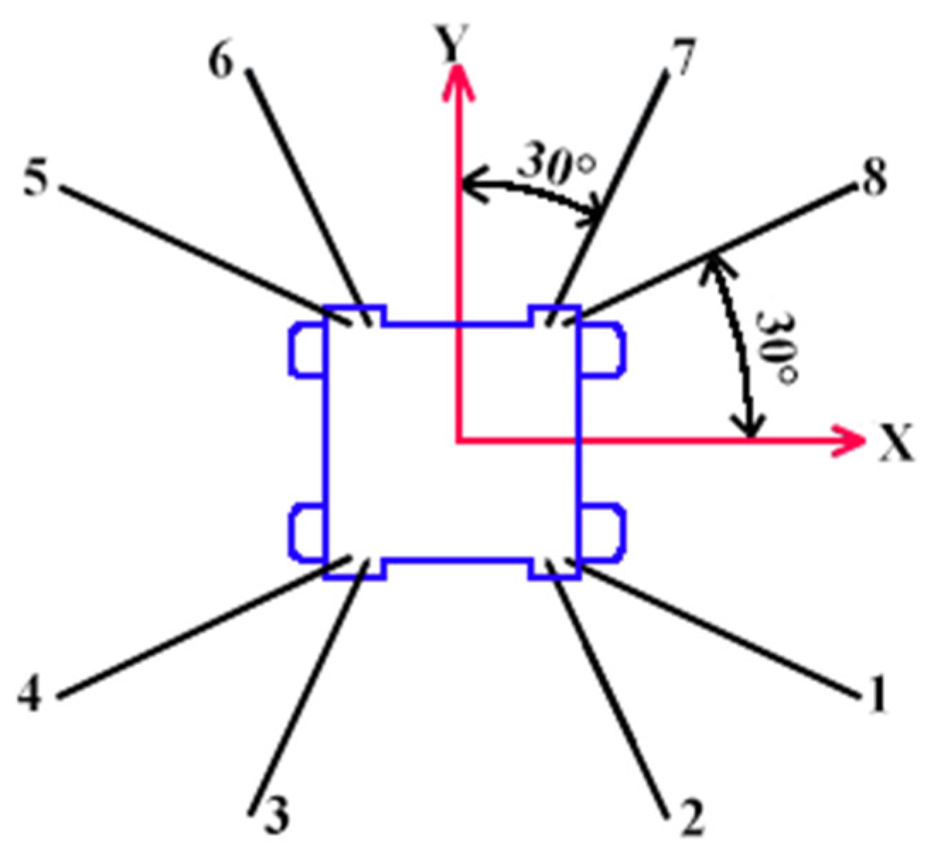
The arrangement of mooring lines in the mooring-aided positioning system is shown in
Figure 1. According to the study of Zhou [
33], the optimal arrangement of mooring lines for this mooring positioning system is that two adjacent mooring lines are 30°, and the angle between one mooring line and the adjacent axis is 30°. Under various wind and wave angles, the platform will not have significant deviation and can maintain high positioning accuracy with directional balance. The water depth is 1500 m. The lengths of the bottom mooring line, intermediate polyester line and top mooring line are 1850 m, 2650 m and 150 m, respectively. The pre-tension of the mooring line is 872 kN. The coordinates of each anchor are depicted in
Table 2. The parameters of the sea environment are as follows. The wave spectrum is JONSWAP, the significant wave height is 3.27 m, the spectral peak period is 13.4 s, the spectral peak factor is 3.3 and the wind and current speeds are 7 m/s and 0.65 m/s, respectively.
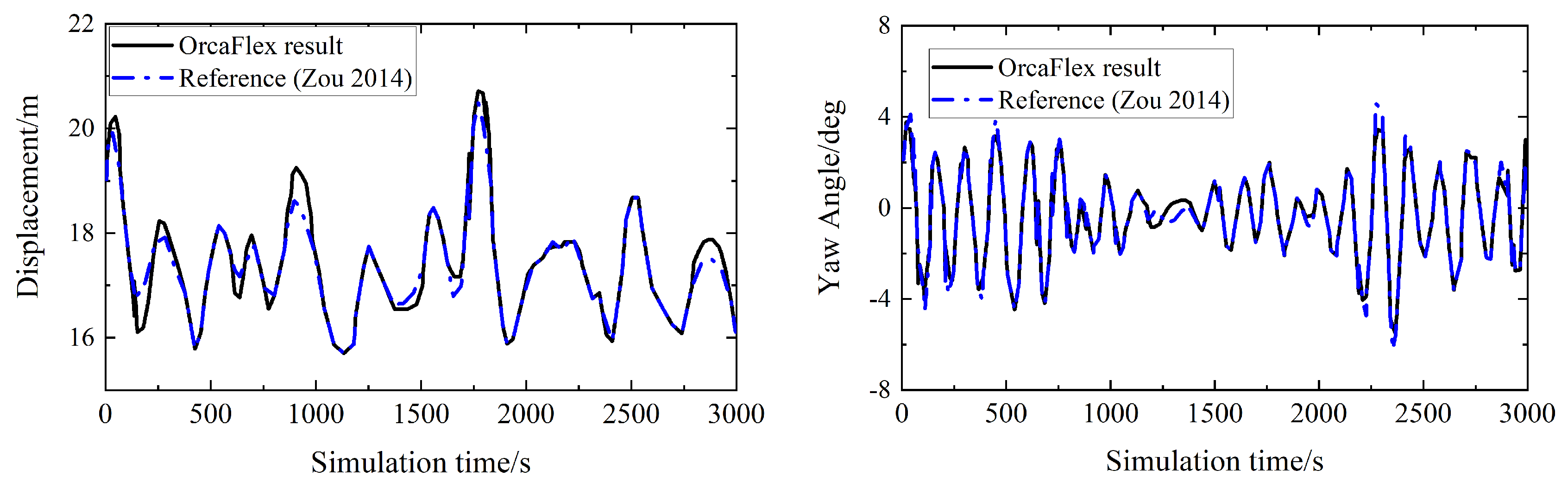
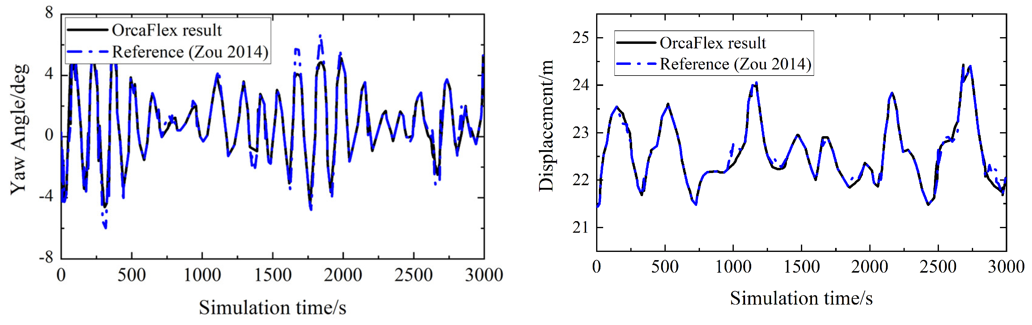
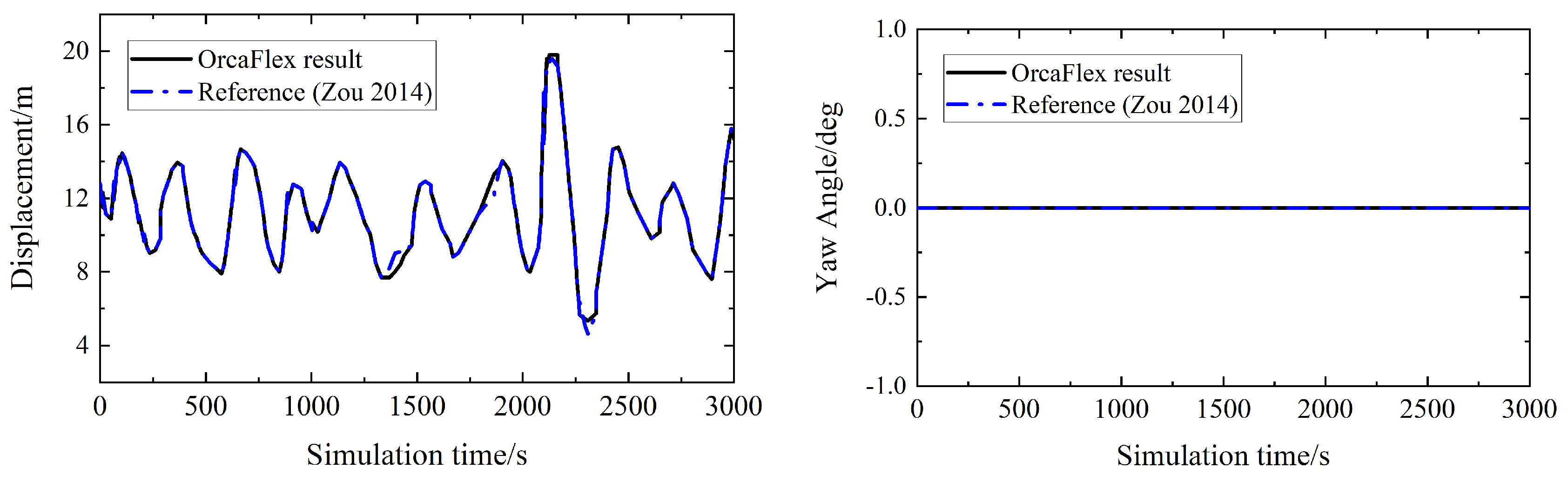
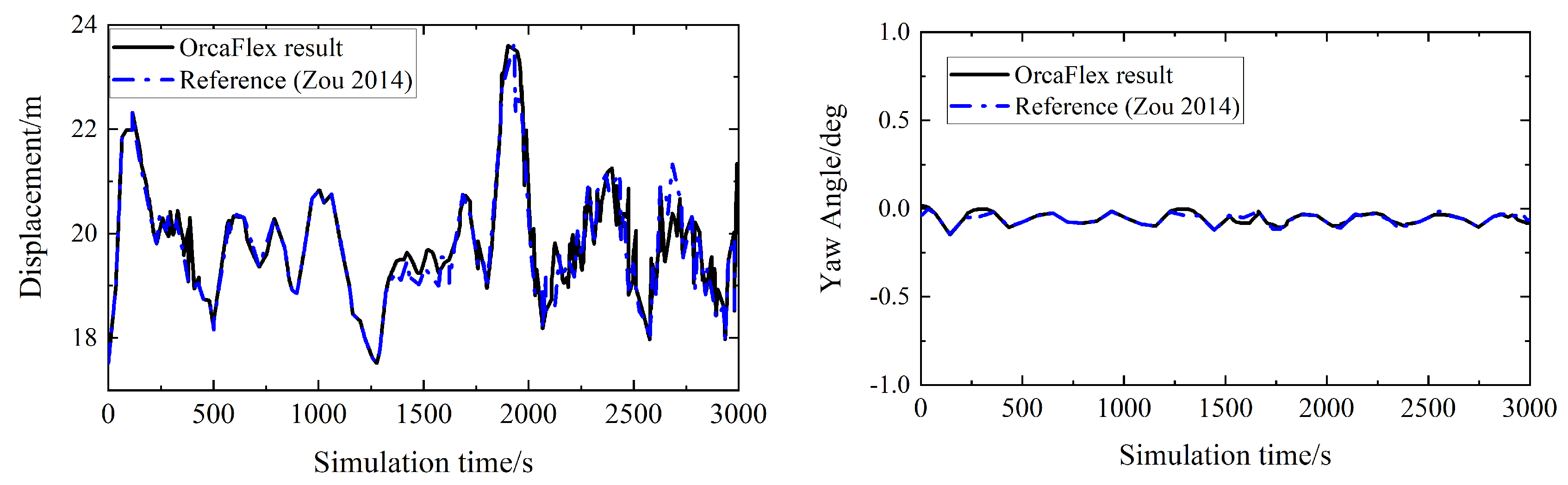
The time domain simulation was carried out with a simulation time of 3000 s. The same directions of wind, waves and currents are selected. Since the mooring positioning system is symmetrically arranged and the platform is also symmetrical, four directions of 180°, 150°, 120° and 90° are selected as the environmental load directions.
Figure 2,
Figure 3,
Figure 4 and
Figure 5 depict the horizontal distance of platform deviation from target position (named Displacement in
Figure 2,
Figure 3,
Figure 4 and
Figure 5) and the yaw angle under four directions. The numerical results are compared with the reference [
33]. It can be seen from
Figure 2,
Figure 3,
Figure 4 and
Figure 5 that the numerical results obtained by OrcaFlex are in good agreement with the reference. In the case of mooring positioning, oblique winds, waves and currents will cause a significant yaw angle of the platform; therefore, the errors become larger. The platform positioned by the mooring system cannot adjust the operating direction, which makes it necessary to assist the mooring system in controlling the heading through thrusters. This is the focus of this paper.
4. Numerical Model Set-Up
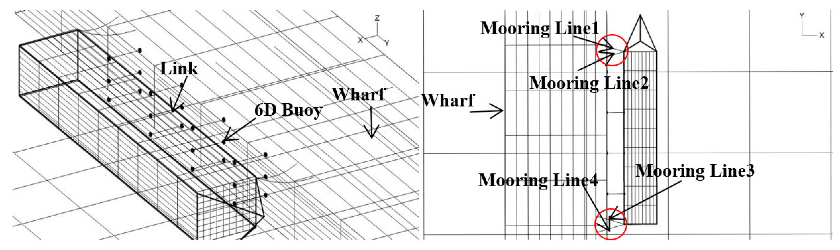
Figure 6 depicts the wharf-cable-dynamic positioning vessel model.
Table 1 shows the vessel’s specifications without a DP system. The global coordinate system is G-xyz, where G is the origin and Gx, Gy and Gz are the X-, Y- and Z-axes. The directions of the external loads are in accordance with the G coordinate system. The defenders in this OrcaFlex simulation model are comprised of 6D buoys (black dots) and Link units (white lines). In
Figure 6, the 12 pairs of dots joined by a line in the x direction are fenders. Four mooring lines connect the ship and wharf. The Link unit is used as a spring damper to connect with a 6D buoy to simulate the dock fender.
Table 3 lists dynamic positioning vessel characteristics. When a collision occurs between the vessel and the wharf, the dock fender might serve as a buffer. The nonlinear stiffness of the Link unit is employed in the calculation of the contact force of the dock fender to ensure effective contact between the vessel and wharf. The reaction force of the fender increases nonlinearly when the distance between the vessel and the wharf is less than a certain value. The force of the Link unit might be insignificant in other circumstances.
The non-linear contact force
T of the fender can be written as:
L is the length of the Link unit when L < L0, the contact force is 0; when 0 m < L < 0.7 m, k = 10/L; when 0.7 m < L < 5 m, k = 1/L; when 5 m < L < 30 m, k = 0.1/L. L0 is taken as 5 m in Equation (8). When L < 5 m, the numerical value of T is negative, which means that the impact of the vessel and wharf occurs.
The lumped mass method is used to calculate the mooring tension of the mooring lines. A single massless model section with nodes at either end describes each line segment of the mooring line. Segments solely model axial and torsional features. The lumped mass approach compares the mooring cable to a nonlinear spring by lumping all other properties to the nodes. This serves as the mathematical foundation for developing the mooring line model in this study [
34]. The parameters of each mooring line are as follows: The inner and outer diameters are 0.25 and 0.35 m; the axial and bending stiffness are 700,000 and 120 kN·m
2; the torsional stiffness, line density, Poisson’s ratio υ and length are 80 kN·m
2, 0.18 t/m, 0.5 and 17 m, respectively.
5. Results and Discussion
Table 4 displays the environmental load parameters. The sea depth is 15 m. The vessel’s reaction will be more severe when the waves, wind and currents are all moving in the same direction. The findings of the calculation may be more greatly affected by environmental load as a result. Therefore, in order to reflect the calculation clearly and make it more convenient to observe, the directions of the waves, wind and currents are in the same direction in the simulation model.
5.1. Comparison of Numerical Results for Non-Dynamic Positioning Vessel vs. Dynamic Positioning Vessel under Mooring
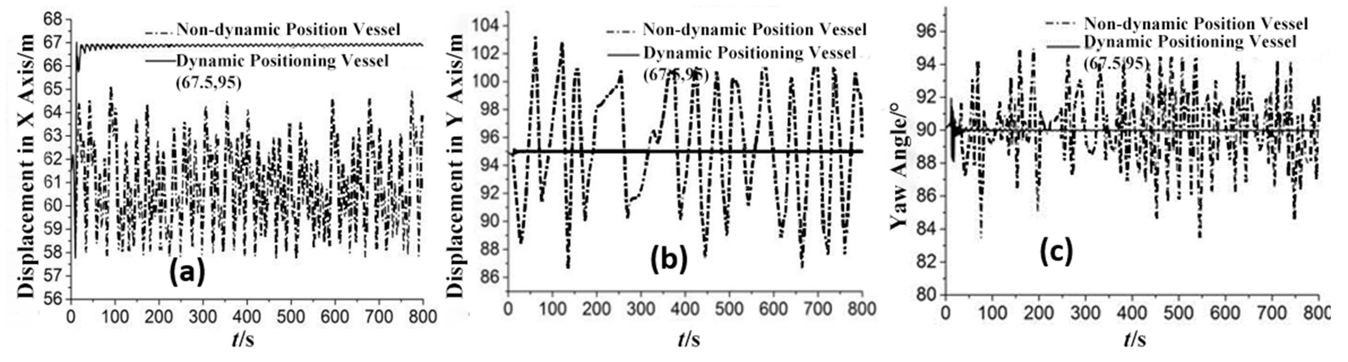
Figure 7 shows the intended location of the dynamic positioning vessel (67.5, 95). Variations in the dynamic positioning vessel’s location and yaw angle are negligible, as shown by the horizontal degrees of freedom motion curves in
Figure 7. As its thruster does not confine the non-dynamic positioning vessel, it has a wider range of motion in the horizontal three DOF. When compared to a moored state, the coupling impact between the different degrees of freedom is much stronger when the vessel is engaged in dynamic positioning. The DP vessel is subsequently stabilized at 67 + 0.05 m in the X-axis direction to restrict the wharf, mooring cable and thruster. Under the influence of external stresses such as wind, waves and currents, the non-dynamic vessel’s displacement in the X-axis exceeds 58 m (27 collisions with the wharf). The DP vessel successfully overcomes the offset induced by the second-order wave drift force along the Y-axis under the influence of the side thruster, stabilizing at 95 ± 0.003 m. The imbalanced distribution of the mooring tension in the Y-axis direction occurs for the non-dynamic positioning vessel when there is a significant range of motion in the X-axis direction. The mooring tension imbalance increases the degree of coupling between the motion along the X- and Y-axes, which has caused instability in the vessel’s whole motion, including the rotational motion of the yaw.
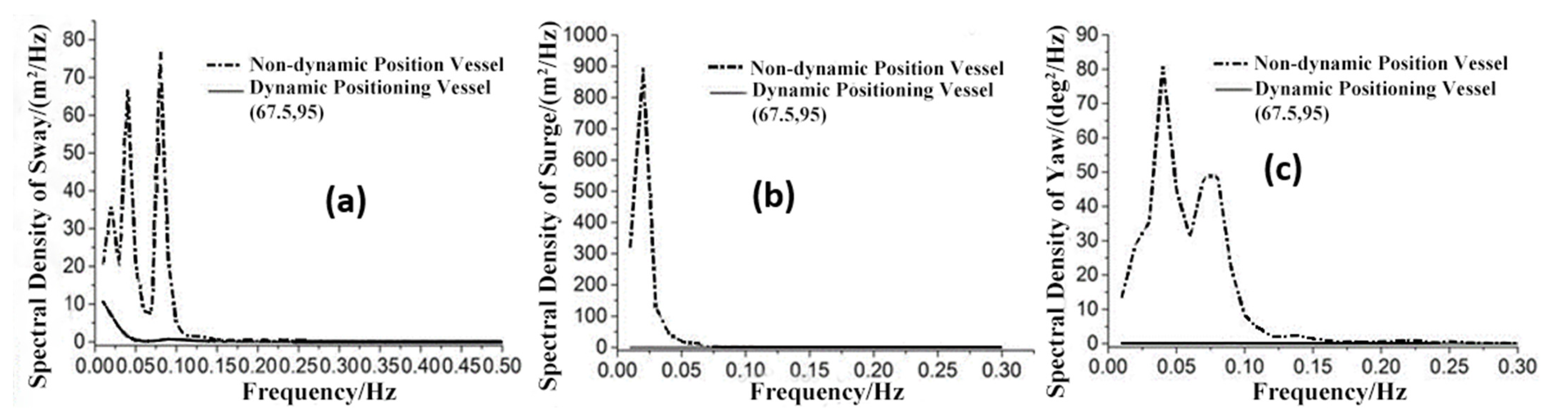
Figure 8 shows the curves for the spectral density of the horizontal degrees of freedom. The spectral density of the DP vessel’s horizontal degrees of freedom is lower than that of the non-dynamic positioning vessel (NDPV) by comparing the curves of spectral density of each degree. The peaks of NDPV sway spectral density rise in the direction of the X-axis, and its low-frequency peaks are mostly dispersed at 0.02 Hz and 0.04 Hz. The wharf constraints, the mooring cable, the second-order wave drift force and the wind and current loads are the primary drivers of the low-frequency components of NDPV. When T = 12 s is the time of the first-order wave force, then the high frequency peak of the non-dynamically located vessel is at 0.08 Hz.
The side thruster’s action during mooring can effectively eliminate the motion component brought on by the first-order wave force in the sway direction, as shown by the DPV peak value of the sway spectral density, which is only at 0.02 Hz and is much smaller than that of the NDPV at the same frequency. The non-dynamic positioning vessel’s surge has a far larger spectral density in the Y-axis direction than it does in the X-axis direction, peaking at 0.025 Hz. As can be observed, movements between various directions exhibit a substantial coupling effect under the impact of the second-order wave drift force and other external loads. This effect is most pronounced in the Y-axis direction. The NDPV peak values in the yaw spectral density curves occur at 0.045 Hz and 0.08 Hz, respectively. The DPV yaw spectrum density, in comparison, is almost negligible. As a result, the lateral thrust reaction force and the wharf-mooring cable may effectively constrain the yaw motion.
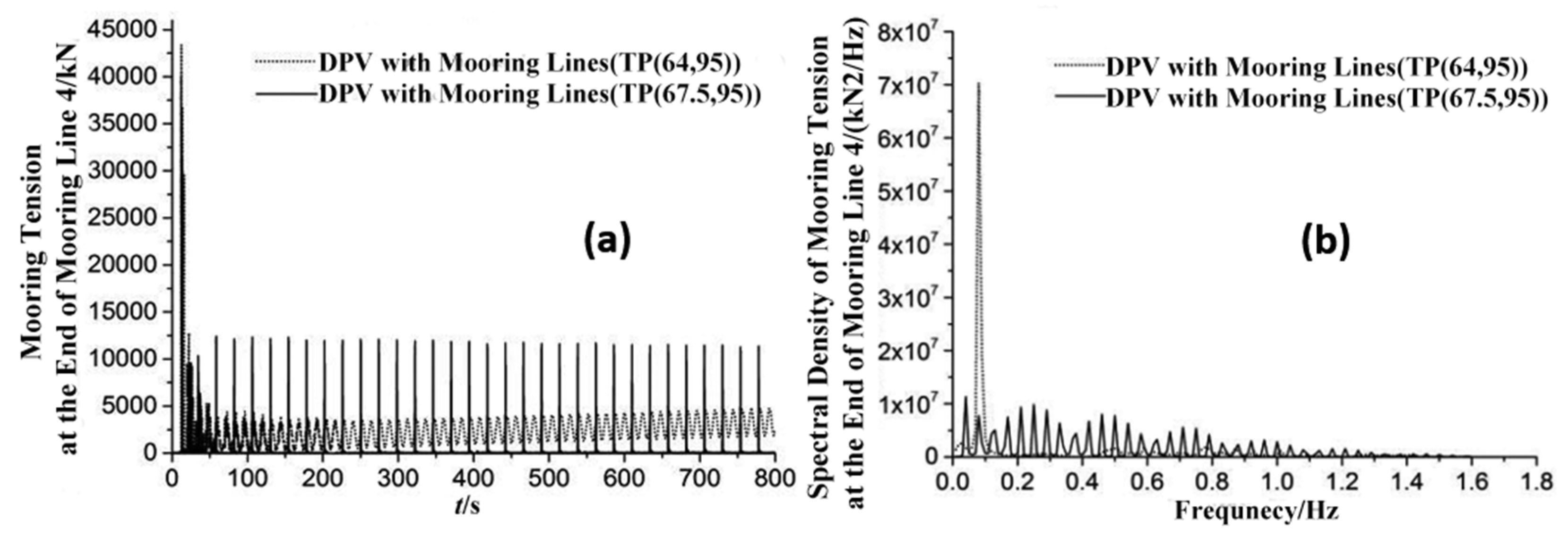
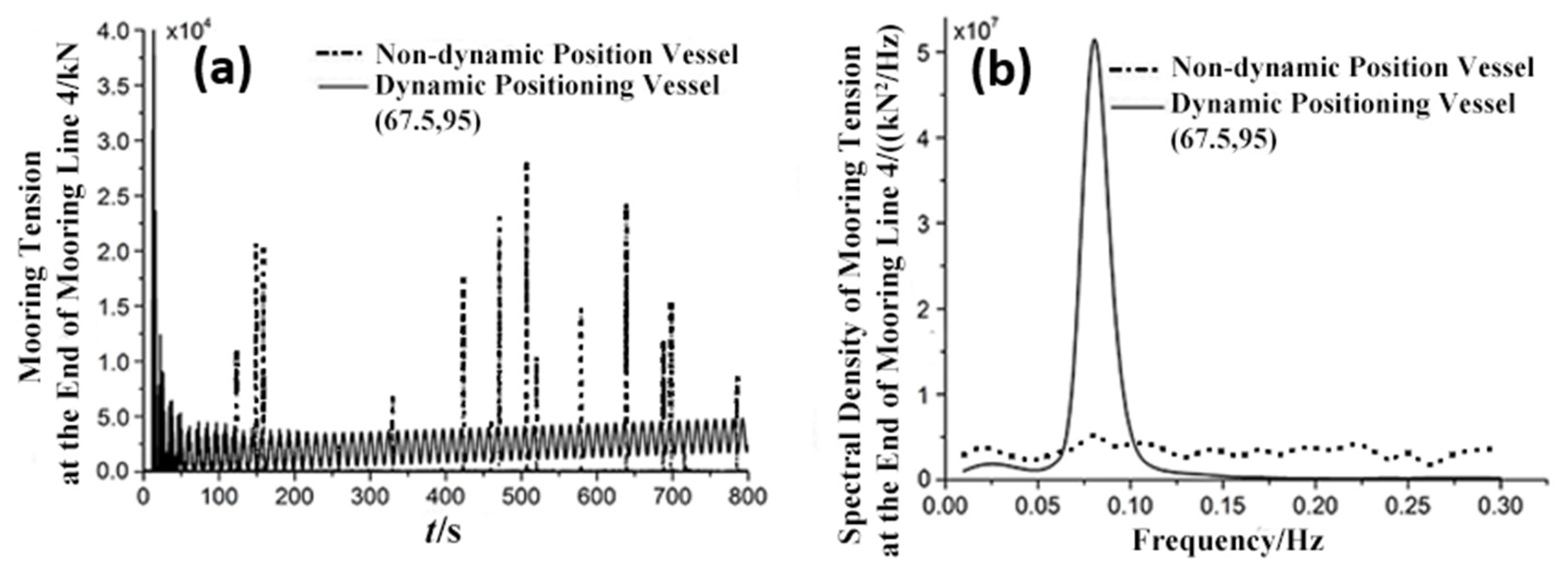
The design of the mooring lines is symmetrical, and their end mooring tension is similarly comparable. Consequently, using Mooring Line 4 as an example, the time-frequency properties of mooring tension at its end are examined in
Figure 9. The mooring tension exhibits an unexpectedly abrupt changing trend in the time domain. This change increases the possibility of the mooring line collapsing due to the quick shift in strain. For the DPV, on the other hand, the side thruster can maintain Mooring Line 4 at a certain tension level. When the direction of wave force (including the second-order wave drift force) is opposite to the direction of mooring tension at Mooring Line 4, the pre-tension effectively offsets the ship motion caused by the first-order wave force. Simultaneously, the mooring tension at the end of Mooring Line 4 gradually increases. The mooring tension at the end of Mooring Line 4 steadily diminishes when the wave force and the mooring tension are in the same direction. During the stage of 0–800 s, the DPV horizontal three DOF motion is maintained within a very small range, as shown in
Figure 7 and
Figure 8. This suggests that the lateral thrust of the side thruster can convert the irregular motion of the vessel at horizontal three degrees of freedom into a regular change in mooring tension in time. At the end of Mooring Line 4, a non-dynamic positioning vessel’s mooring tension spectral density is evenly distributed between 0.0 Hz and 0.3 Hz, and the frequency band of its motion is nonlinear. At the end of a DPV Mooring Line 4, the optimum mooring tension is 0.08 Hz, which corresponds to the wave frequency. This shows that the side thruster’s pretension on the mooring line counteracts the force of the first-order wave load on the ship. This implies that the three horizontal degrees of freedom remains within a very small range of motion.
5.2. Numerical Comparison of Dynamic Positioning Vessels with and without Mooring Lines
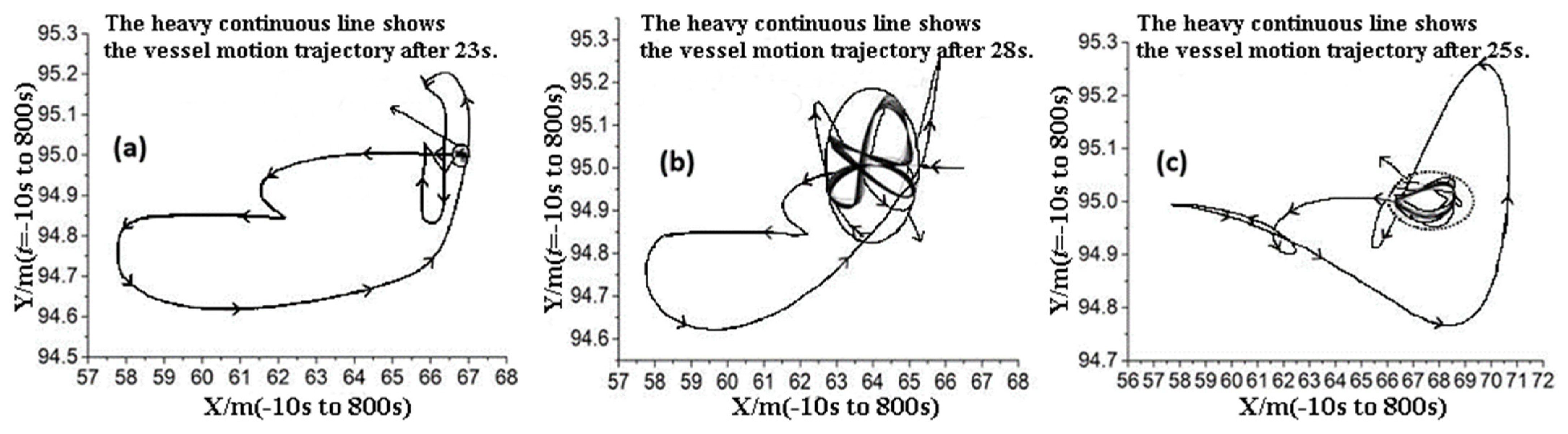
Figure 10a shows the trajectory of DPV (67.5, 95) with mooring lines in the x-y plane, and its motion with mooring lines tends to be stable at the moment of 23 s. The arrow shows the motion direction of the dynamic positioning vessel responds from −10 s to 23 s and at (67.5 ± 0.05, 95 ± 0.003); a stable state was attained. The target dynamic position (64, 95) vessel’s x-y plane mooring line trajectory is also shown in
Figure 5b.
In comparison to the model in
Figure 5a, the time for the vessel in
Figure 10b to reach a stable state is 28 s, and the vessel ultimately stabilizes at (64 ± 2.15, 95 ± 0.29).
Figure 10c depicts the trajectory of a DPV without mooring lines in the x-y plane, with its objective location shown as (67.5, 95.0). The DPV without mooring lines stabilizes at (67.5 ± 2.9, 95 ± 0.09) after stabilizing significantly in comparison to DPV with mooring lines. The heavy continuous line first displays the trajectory of the vessel after 28 s.
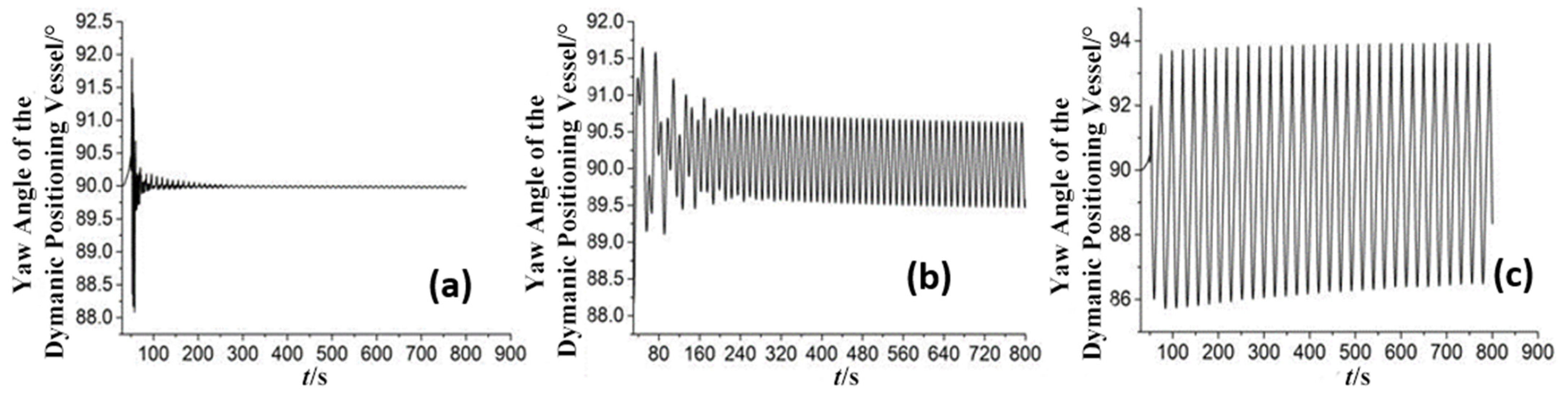
The dynamic positioning vessel’s yaw angle curves (with and without mooring lines) in the time domain for the identical environmental loads are shown in
Figure 11. The target position (TP) denotes the target x-y coordinates for the DPV. The yaw angle of the vessel experiences an increase in amplitude from
Figure 11a–c. It can be observed that the mooring lines limit the motion of the vessel’s yaw when comparing the yaw angles of DPV with mooring lines with DPV without mooring lines. As a result, the DPV with mooring lines has far less of a change in yaw angle than the dynamic positioning vessel without mooring lines.
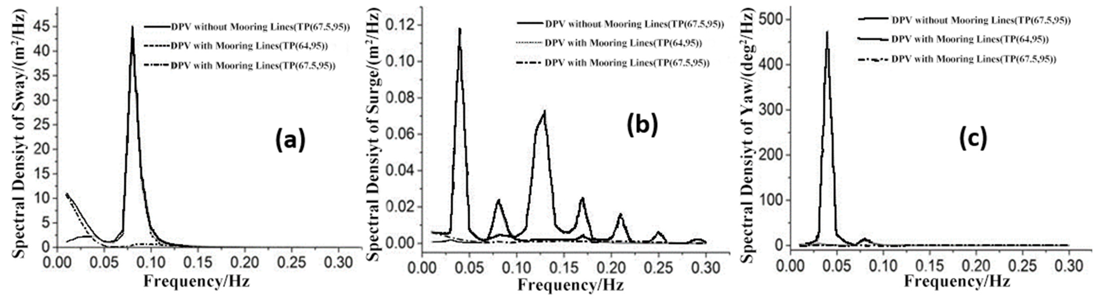
Figure 12 illustrates the spectral density of the vessel’s horizontal three degrees of freedom. The vessel sway spectral density curves for the DPV without mooring lines (TP (67.5, 95)) and the DPV with mooring lines (TP (64, 95)) are determined to be virtually identical. The peak values coincide with the wave load frequency. When a DPV is moored to mooring lines, the peak value of the roll spectral density is drastically lowered to the TP (67.5, 95). The spectral density of the DPV with the mooring lines (TP (64, 95)) is higher. It indicates that the level of motion of the horizontal three degrees of freedom in this state still has a higher degree of coupling, whereas the degree of coupling between the horizontal three degrees of freedom both states is minimal. This is evident by observing the vessel’s surge spectral density and yaw spectral density curves. As a result, the wharf-cable has the potential to enhance the DPV positioning performance, but it is essential is to choose an adequate target position.
Figure 13 illustrates the spectral density curves of mooring tension on Mooring Line 4 of the DPV. Compared to the NDPV with mooring lines in
Figure 9, the DPV with mooring lines (TP (64, 95)) exhibits fewer sudden changes in tension at the end of Mooring Line 4. Nevertheless, Mooring Line 4’s termination point’s spectral density curves still cover a wide frequency range. As a result, when the target position is (64, 65), the target position selection is unreasonable, resulting in the mooring lines being unable to be tensioned at all times. There is not enough tension in the mooring lines to offset the power of the wave on the vessel as the wave load pulls it toward the wharf. The mooring lines will experience a greater acceleration displacement when the wave load or the wharf’s collision force pulls the vessel away from the wharf. This will result in a quick change in mooring tension to counteract the vessel’s motion. The peak value of mooring tension spectral density might therefore be guaranteed to be near to the wave external load frequency by a reasonable target position.
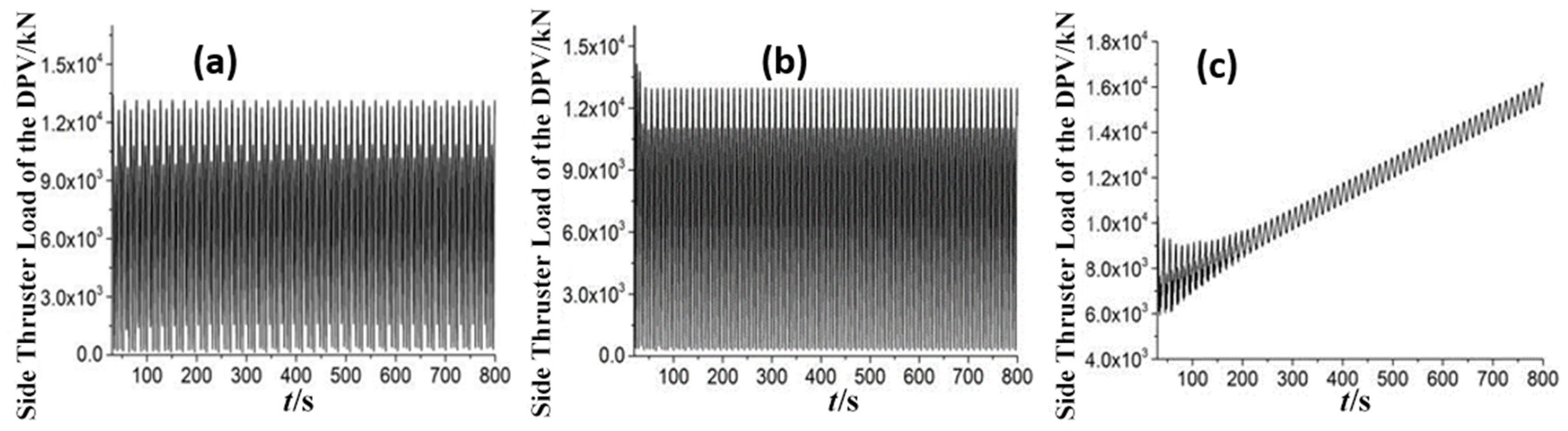
As shown in
Figure 14, the side thruster load of DPV with mooring lines (TP (64, 95)) is basically consistent with the side thruster load of DPV without mooring lines (TP (64, 95)). The side thruster load of the DPV with mooring lines (TP (67.5, 95)) increases with time since the control strategy lacks a program for regulating the maximum thruster power. Compared with
Figure 10, it can be observed that the DPV with mooring lines (TP (67.5, 95)) has been in a stable state for the last 23 s and that the motion amplitude is very small. The addition of the maximum power restriction to the control method is not predicted to alter the results shown in
Figure 10. The DPV with mooring lines (TP (67.5, 95)) side thruster load has the minimum amplitude of thrust fluctuation. When the thruster power limiter software is installed, the thrust will always be maintained within a predetermined range.
The peak values of side thruster load spectral density curves of DPV with mooring lines (TP (64, 95)) and the DPV without mooring lines (TP (64, 95)) are all distributed within the range of high frequency. Contrarily, the DPV with mooring lines (TP (67.5, 95)) shows a spectral density curve with a peak value near a low frequency for load on the side thrusters. In practical engineering, a high-frequency load shift will severely damage the side thruster and the dynamic positioning system. Hence, the frequency of the thrust of the DPV could be effectively reduced in the frequency domain, provided that a suitable goal position is selected, and mooring lines are utilized adequately.
6. Conclusions
In the mooring state, the time-frequency features of the horizontal three DOF (degrees of freedom) motion of the vessel and the mooring tension of the mooring line are compared, and the side thruster in the coupled system’s effect on the elimination of vessel motion caused by the first-order wave l was examined. The effect of the wharf-cable and target position on the side thruster of DPV was determined by comparing its performance with and without mooring lines under the same environmental stress. The performance of the NDPV and DPV with mooring lines under the same environmental load was compared. The influence of the side thruster in coupled systems on the elimination of vessel motion caused by first-order wave load is analyzed. Non-dynamic positioning vessels have a greater spectral density in the horizontal three degrees of freedom due to a stronger coupling between their degrees of freedom. As a result of the connection, the mooring tension shifts abruptly, and the spectral density is spread out evenly. DP systems are weak to cancel linear wave forces, and the missing ship motions for DP ships may be due to the combined action of the fender, moorings and the selection of a good target position. When the selection of the target position is unreasonable, the size of the pre-tension of the mooring line cannot meet the requirement of absorbing the first-order wave load on the vessel. When the target moves closer to its true location, the frequency with which the horizontal thrust load shifts decreases, the side thruster’s work efficiency increases and the coupling system’s safety increases.
In particular, to simplify the numerical model, the impact of gap flow between a ship and a wharf was not estimated, which is a deficiency of this paper. With OrcaFlex, harmonic analysis with RAO or multibody analysis was performed after entering the hydrodynamic coefficients. Future research will focus on the calculation of co-hydrodynamic forces due to interstitial flows.


