

A Simplified Experimental Method to Estimate the Transport of Non-Buoyant Plastic Particles Due to Waves by 2D Image Processing


Abstract
:1. Introduction
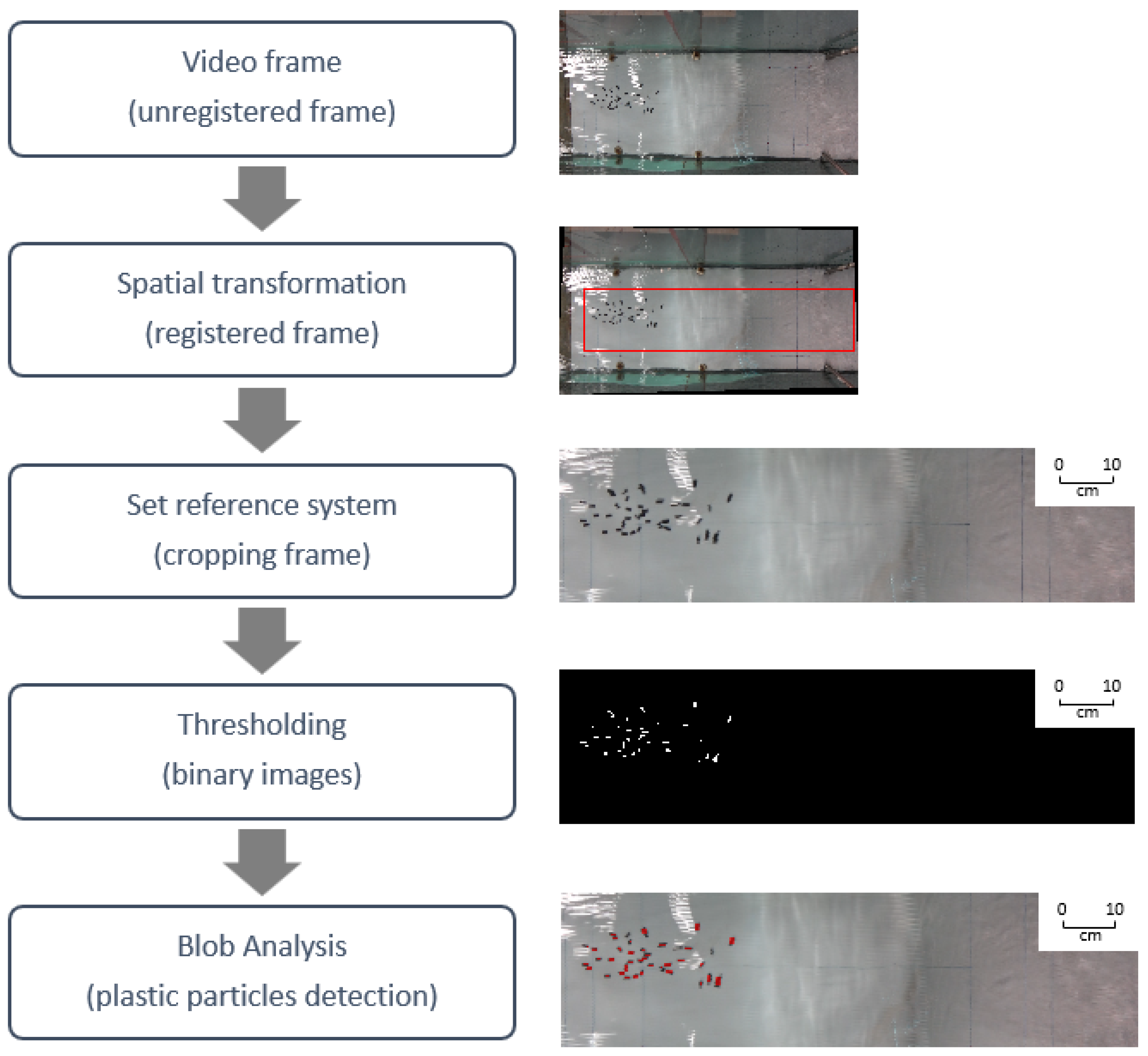
2. Video Recording Processing Algorithm
2.1. Algorithms for Frame Analysis
2.2. Characteristic Parameters of Plastic Debris Displacement
3. Experimental Procedure
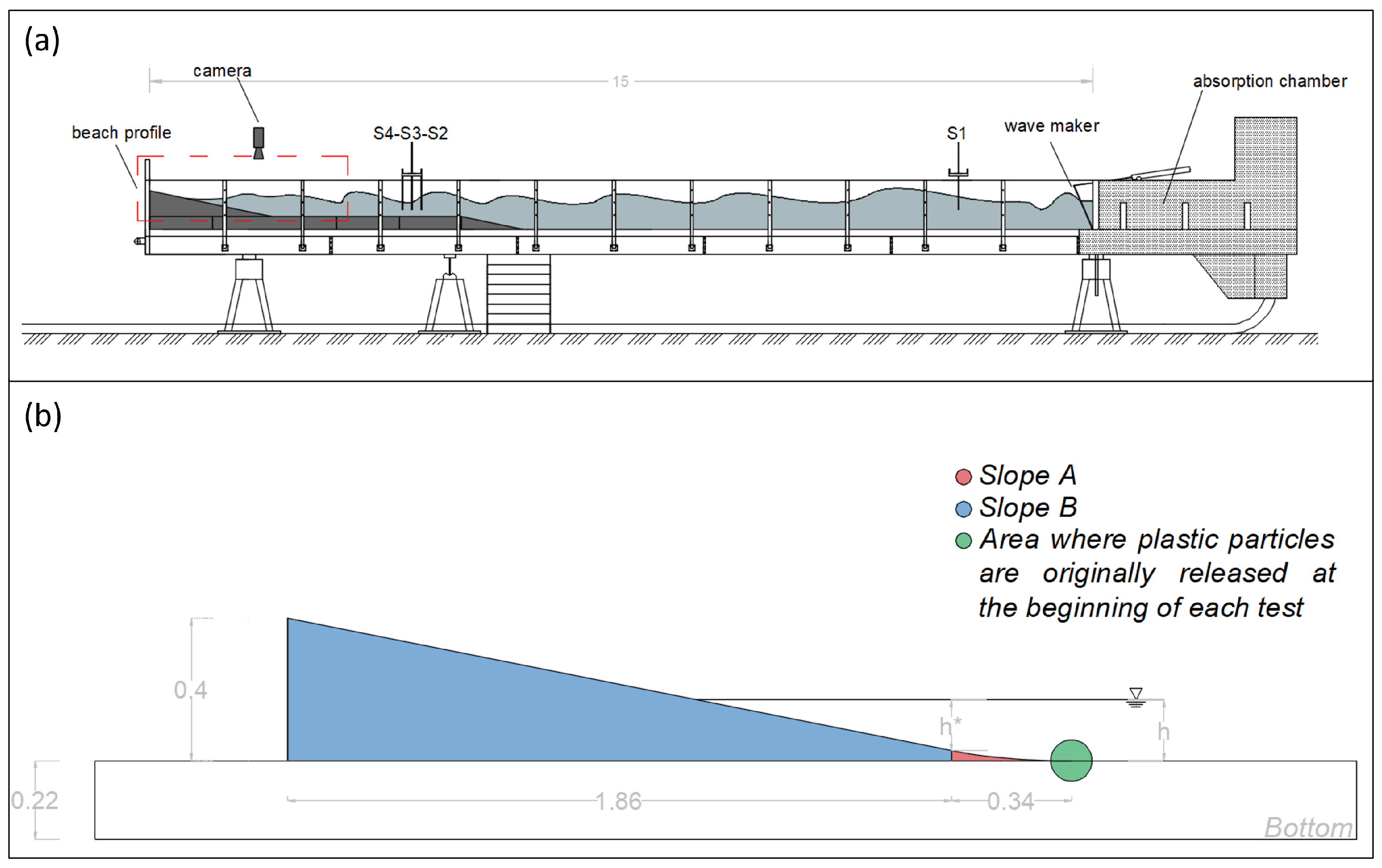
3.1. Laboratory Equipment
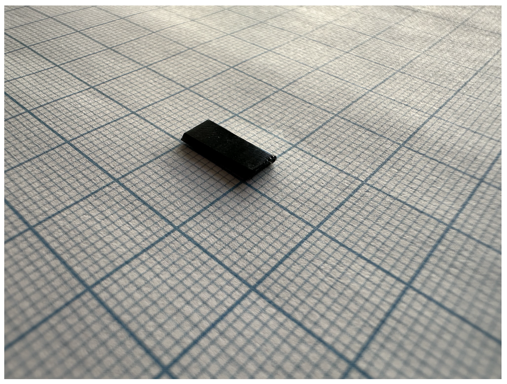
3.2. Plastic Particles
4. Experiments
5. Results
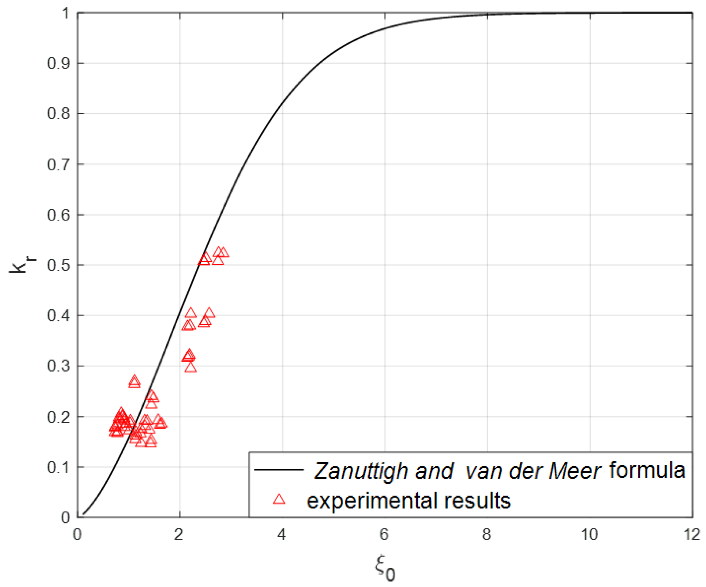
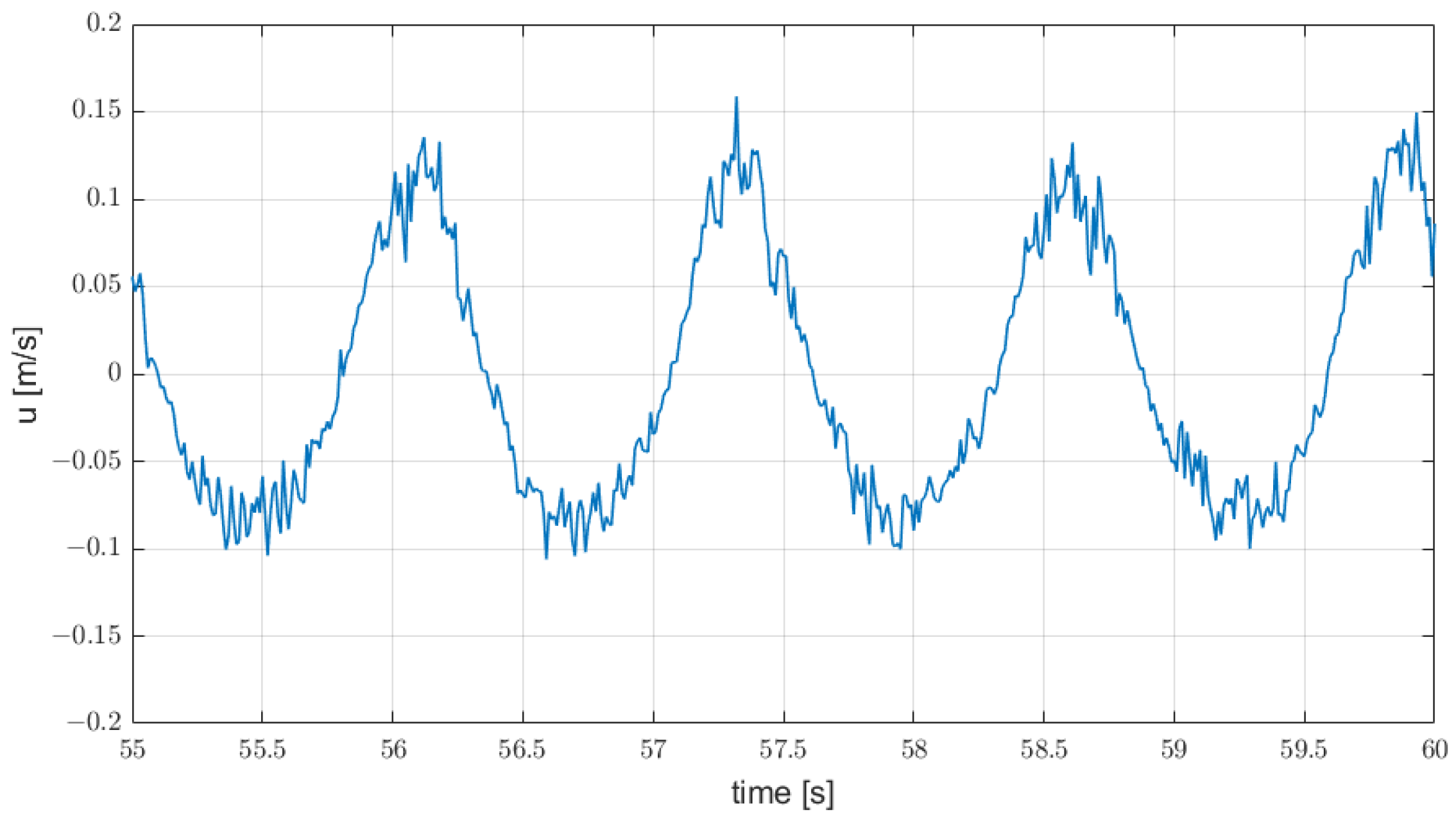
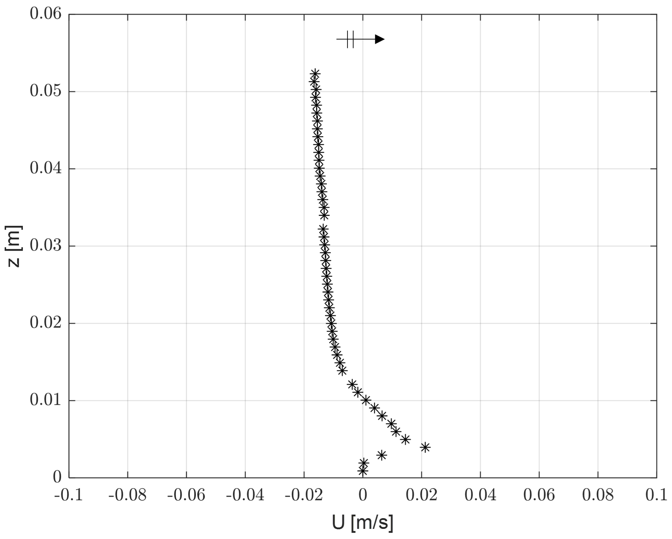
5.1. Flow Velocity
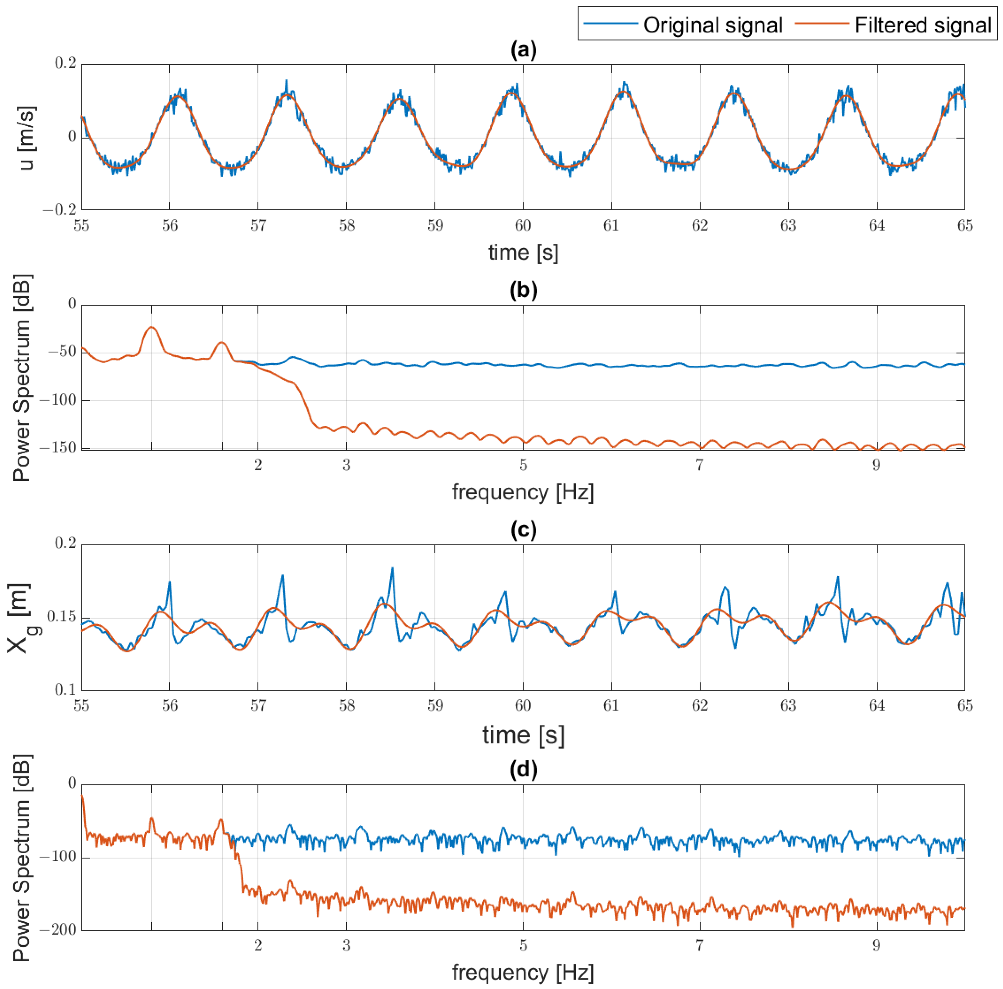
5.2. Validation of Spatial Transformation
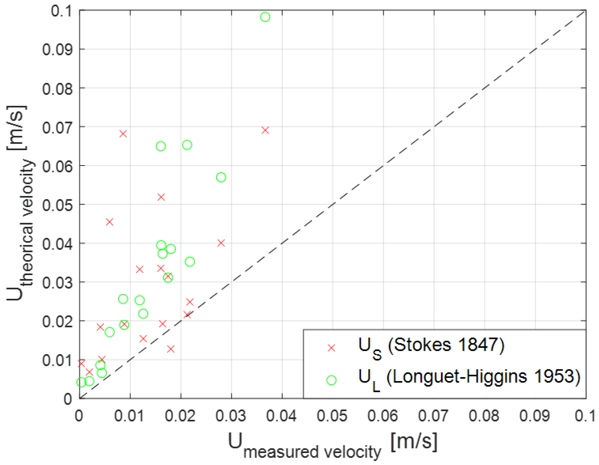
5.3. Calibration of Velocity Measurement
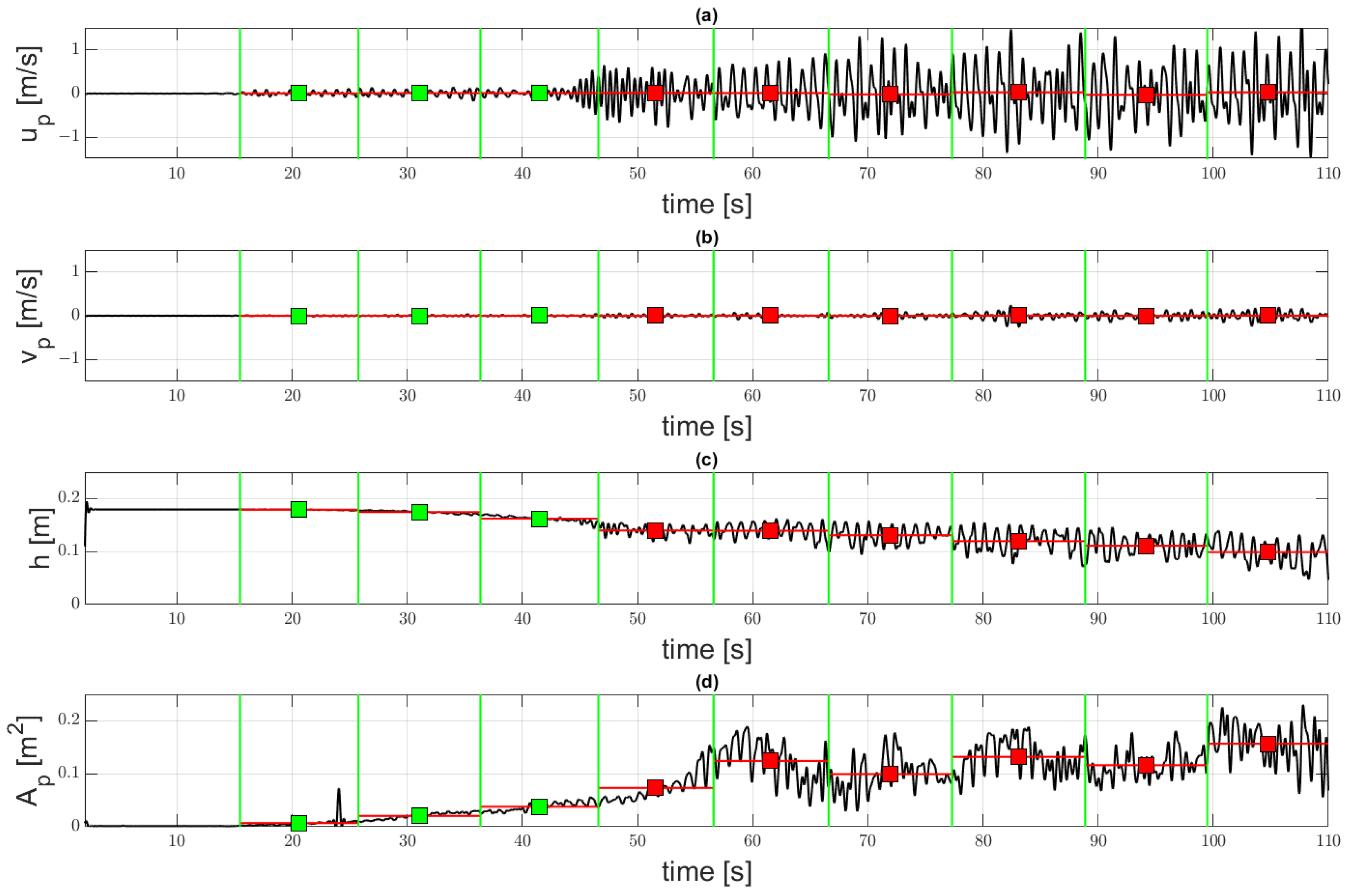
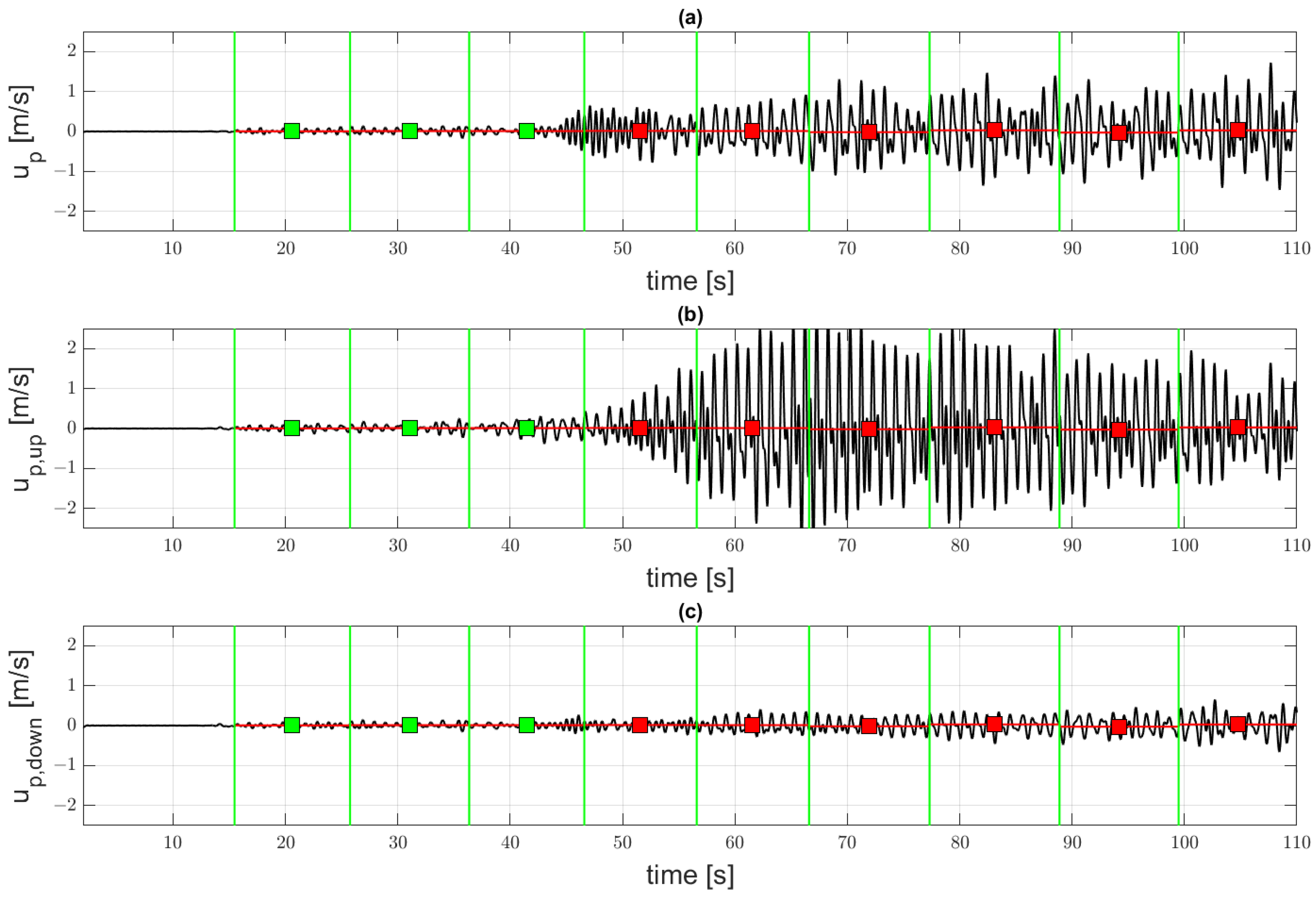
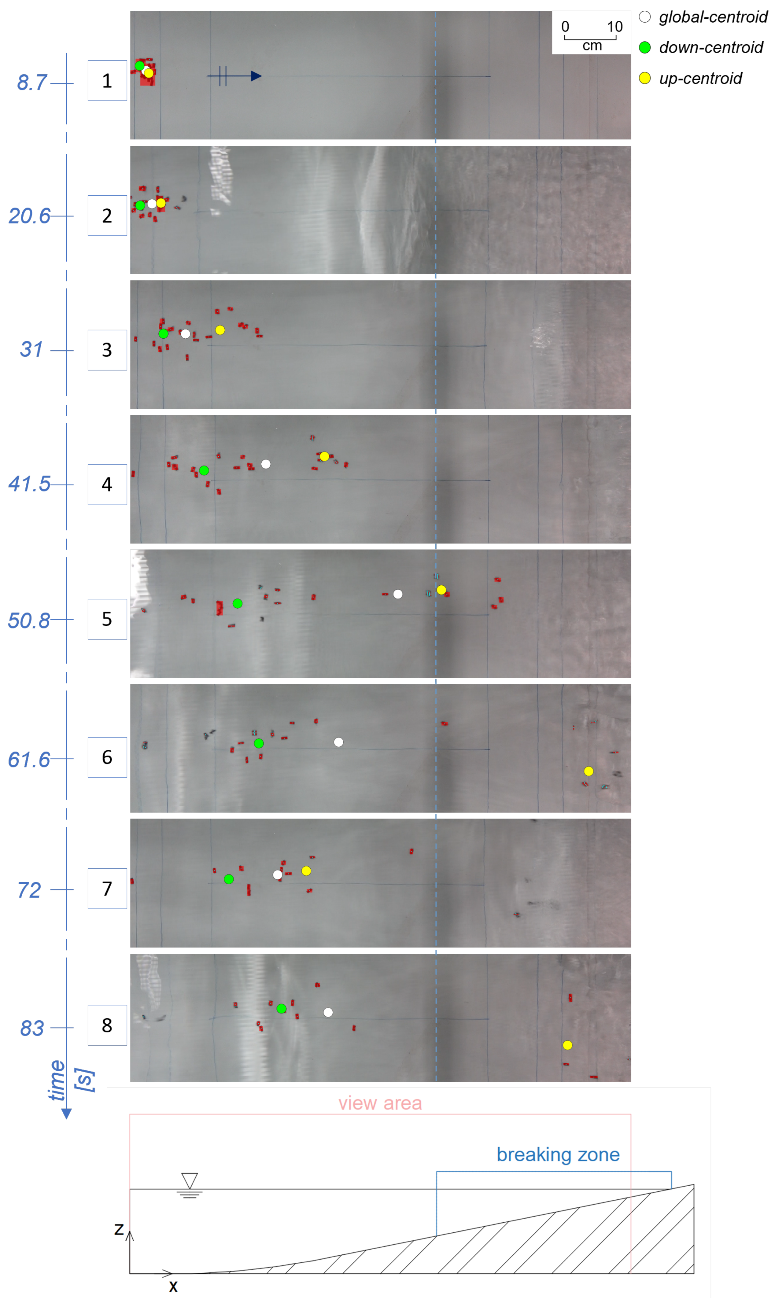
5.4. Plastic Particles Velocity Analysis
6. Conclusions
Author Contributions
Funding
Institutional Review Board Statement
Informed Consent Statement
Data Availability Statement
Conflicts of Interest
References
- Smith, J.K., Jr. World War II and the transformation of the American chemical industry. In Science, Technology and the Military; Springer: Berlin/Heidelberg, Germany, 1988; pp. 307–322. [Google Scholar]
- LI, W.C.; Tse, H.; Fok, L. Plastic waste in the marine environment: A review of sources, occurrence and effects. Sci. Total Environ. 2016, 566, 333–349. [Google Scholar] [CrossRef] [PubMed]
- Jambeck, J.R.; Geyer, R.; Wilcox, C.; Siegler, T.R.; Perryman, M.; Andrady, A.; Narayan, R.; Law, K.L. Plastic waste inputs from land into the ocean. Science 2015, 347, 768–771. [Google Scholar] [CrossRef]
- Ederer, B.; Sluka, R.D. Plastics in the Food Chain. Perspect. Sci. Christ. Faith 2020, 72, 169–170. [Google Scholar]
- Amran, N.H.; Zaid, S.S.M.; Mokhtar, M.H.; Manaf, L.A.; Othman, S. Exposure to Microplastics during Early Developmental Stage: Review of Current Evidence. Toxics 2022, 10, 597. [Google Scholar] [CrossRef] [PubMed]
- Klavins, M.; Klavins, L.; Stabnikova, O.; Stabnikov, V.; Marynin, A.; Ansone-Bertina, L.; Mezulis, M.; Vaseashta, A. Interaction between Microplastics and Pharmaceuticals Depending on the Composition of Aquatic Environment. Microplastics 2022, 1, 520–535. [Google Scholar] [CrossRef]
- Critchell, K.; Lambrechts, J. Modelling accumulation of marine plastics in the coastal zone; what are the dominant physical processes? Plast. Food Chain. 2016, 171, 111–122. [Google Scholar] [CrossRef]
- Zhang, H. Transport of microplastics in coastal seas. Plast. Food Chain. 2017, 199, 74–86. [Google Scholar] [CrossRef]
- Van Sebille, E.; Aliani, S.; Law, K.L.; Maximenko, N.; Alsina, J.M.; Bagaev, A.; Bergmann, M.; Chapron, B.; Chubarenko, I.; Cózar, A.; et al. The physical oceanography of the transport of floating marine debris. Environ. Res. Lett. 2020, 15, 023003. [Google Scholar] [CrossRef]
- Stocchino, A.; De Leo, F.; Besio, G. Sea waves transport of inertial micro-plastics: Mathematical model and applications. J. Mar. Sci. Eng. 2019, 7, 467. [Google Scholar] [CrossRef]
- Lebreton, L.C.; Van Der Zwet, J.; Damsteeg, J.W.; Slat, B.; Andrady, A.; Reisser, J. River plastic emissions to the world’s oceans. Nat. Commun. 2017, 8, 15611. [Google Scholar] [CrossRef]
- Waldschläger, K.; Schüttrumpf, H. Erosion behavior of different microplastic particles in comparison to natural sediments. Environ. Sci. Technol. 2019, 53, 13219–13227. [Google Scholar] [CrossRef]
- Lentz, S.J.; Fewings, M.R. The wind-and wave-driven inner-shelf circulation. Annu. Rev. Mar. Sci. 2012, 4, 317–343. [Google Scholar] [CrossRef]
- Kerpen, N.B.; Schlurmann, T.; Schendel, A.; Gundlach, J.; Marquard, D.; Hüpgen, M. Wave-induced distribution of microplastic in the surf zone. Front. Mar. Sci. 2020, 7, 590565. [Google Scholar] [CrossRef]
- Forsberg, P.L.; Sous, D.; Stocchino, A.; Chemin, R. Behaviour of plastic litter in nearshore waters: First insights from wind and wave laboratory experiments. Mar. Pollut. Bull. 2020, 153, 111023. [Google Scholar] [CrossRef]
- Alsina, J.M.; Jongedijk, C.E.; van Sebille, E. Laboratory Measurements of the Wave-Induced Motion of Plastic Particles: Influence of Wave Period, Plastic Size and Plastic Density. J. Geophys. Res. Ocean. 2020, 125, e2020JC016294. [Google Scholar] [CrossRef]
- Larsen, B.E.; Al-Obaidi, M.A.A.; Guler, H.G.; Carstensen, S.; Goral, K.D.; Christensen, E.D.; Kerpen, N.B.; Schlurmann, T.; Fuhrman, D.R. Experimental investigation on the nearshore transport of buoyant microplastic particles. Mar. Pollut. Bull. 2023, 187, 114610. [Google Scholar] [CrossRef]
- Petrotta, C.; Faraci, C.; Scandura, P.; Foti, E. Experimental investigation on sea ripple evolution over sloping beaches. Ocean. Dyn. 2018, 68, 1221–1237. [Google Scholar] [CrossRef]
- Faraci, C.; Scandura, P.; Petrotta, C.; Foti, E. Wave-induced oscillatory flow over a sloping rippled bed. Water 2019, 11, 1618. [Google Scholar] [CrossRef]
- DiBenedetto, M.H.; Ouellette, N.T.; Koseff, J.R. Transport of anisotropic particles under waves. J. Fluid Mech. 2018, 837, 320–340. [Google Scholar] [CrossRef]
- Longuet-Higgins, M.S. Mass transport in water waves. Philos. Trans. R. Soc. London Ser. A Math. Phys. Sci. 1953, 245, 535–581. [Google Scholar]
- Scandura, P.; Foti, E.; Faraci, C. Mass transport under standing waves over a sloping beach. J. Fluid Mech. 2012, 701, 460–472. [Google Scholar] [CrossRef]
- Pezerat, M.; Bertin, X.; Martins, K.; Lavaud, L. Cross-shore distribution of the wave-induced circulation over a dissipative beach under storm wave conditions. J. Geophys. Res. Ocean. 2022, 127, e2021JC018108. [Google Scholar] [CrossRef]
- Bijker, E.; Kalwijk, J.T.; Pieters, T. Mass transport in gravity waves on a sloping bottom. In Proceedings of the 14th Conference on Coastal Engineering, Copenhagen, Denmark, 24–28 June 1974; pp. 447–465. [Google Scholar]
- Turner, I.L.; Russell, P.E.; Butt, T. Measurement of wave-by-wave bed-levels in the swash zone. Coast. Eng. 2008, 55, 1237–1242. [Google Scholar] [CrossRef]
- Saugy, J.N.; Amini, A.; De Cesare, G. Flow structure and grain motion assessments of large river widening in a physical model using ultrasonic Doppler velocity measurements. Exp. Fluids 2022, 63, 115. [Google Scholar] [CrossRef]
- Radice, A.; Malavasi, S.; Ballio, F. Solid transport measurements through image processing. Exp. Fluids 2006, 41, 721–734. [Google Scholar] [CrossRef]
- Liu, C.; Kiger, K.T. Multi-camera single-plane PIV imaging in two-phase flow for improved dispersed-phase concentration. Exp. Fluids 2022, 63, 41. [Google Scholar] [CrossRef]
- Zimmermann, A.E.; Church, M.; Hassan, M.A. Video-based gravel transport measurements with a flume mounted light table. Earth Surf. Process. Landf. 2008, 33, 2285–2296. [Google Scholar] [CrossRef]
- Núñez, P.; Romano, A.; García-Alba, J.; Besio, G.; Medina, R. Wave-induced cross-shore distribution of different densities, shapes, and sizes of plastic debris in coastal environments: A laboratory experiment. Mar. Pollut. Bull. 2023, 187, 114561. [Google Scholar] [CrossRef]
- Guler, H.G.; Larsen, B.E.; Quintana, O.; Goral, K.D.; Carstensen, S.; Christensen, E.D.; Kerpen, N.B.; Schlurmann, T.; Fuhrman, D.R. Experimental study of non-buoyant microplastic transport beneath breaking irregular waves on a live sediment bed. Mar. Pollut. Bull. 2022, 181, 113902. [Google Scholar] [CrossRef]
- Moeslund, T.B.; Moeslund, T.B. BLOB analysis. In Introduction to Video and Image Processing: Building Real Systems and Applications; Springer: Aalborg, Denmark, 2012; pp. 103–115. [Google Scholar]
- Zhou, H.; Llewellyn, L.; Wei, L.; Creighton, D.; Nahavandi, S. Marine Object Detection Using Background Modelling and Blob Analysis. In Proceedings of the 2015 IEEE International Conference on Systems, Man, and Cybernetics, Hong Kong, 9–12 October 2015; pp. 430–435. [Google Scholar] [CrossRef]
- Chen, T.H.; Lin, Y.F.; Chen, T.Y. Intelligent Vehicle Counting Method Based on Blob Analysis in Traffic Surveillance. In Proceedings of the Second International Conference on Innovative Computing, Information and Control (ICICIC 2007), Kumamoto, Japan, 5–7 September 2007; p. 238. [Google Scholar] [CrossRef]
- Adal, K.M.; Sidibé, D.; Ali, S.; Chaum, E.; Karnowski, T.P.; Mériaudeau, F. Automated detection of microaneurysms using scale-adapted blob analysis and semi-supervised learning. Comput. Methods Programs Biomed. 2014, 114, 1–10. [Google Scholar] [CrossRef]
- Jia, T.; Sun, N.l.; Cao, M.y. Moving object detection based on blob analysis. In Proceedings of the 2008 IEEE International Conference on Automation and Logistics, Qingdao, China, 1–3 September 2008; pp. 322–325. [Google Scholar] [CrossRef]
- Al-Amri, S.S.; Kalyankar, N.V. Image segmentation by using threshold techniques. arXiv 2010, arXiv:1005.4020. [Google Scholar]
- MATLAB, version 9.13.0 (R2022b); The MathWorks Inc.: Natick, MA, USA, 2022.
- Iuppa, C.; Carlo, L.; Foti, E.; Faraci, C. Calibration of CFD Numerical Model for the Analysis of a Combined Caisson. Water 2021, 13, 2862. [Google Scholar] [CrossRef]
- Carlo, L.; Iuppa, C.; Faraci, C. A numerical-experimental study on the hydrodynamic performance of a U-OWC wave energy converter. Renew. Energy 2023, 203, 89–101. [Google Scholar] [CrossRef]
- Mansard, E.P.; Funke, E. The measurement of incident and reflected spectra using a least squares method. In Proceedings of the 17th International Conference on Coastal Engineering, Sydney, Australia, 23–28 March 1980; pp. 154–172. [Google Scholar]
- Corey, A.T. Influence of Shape on the Fall Velocity of Sand Grains. PhD Thesis, Colorado A & M College, Colorado State University, Fort Collins, CO, USA, 1949. [Google Scholar]
- Mistri, M.; Infantini, V.; Scoponi, M.; Granata, T.; Moruzzi, L.; Massara, F.; De Donati, M.; Munari, C. Small plastic debris in sediments from the Central Adriatic Sea: Types, occurrence and distribution. Mar. Pollut. Bull. 2017, 124, 435–440. [Google Scholar] [CrossRef] [PubMed]
- Sharma, S.; Sharma, V.; Chatterjee, S. Microplastics in the Mediterranean Sea: Sources, pollution intensity, sea health, and regulatory policies. Front. Mar. Sci. 2021, 8, 634934. [Google Scholar] [CrossRef]
- Zanuttigh, B.; van der Meer, J.W. Wave reflection from coastal structures in design conditions. Coast. Eng. 2008, 55, 771–779. [Google Scholar] [CrossRef]
- Stokes, G.G. On the theory of oscillatory waves. Trans. Cam. Philos. Soc. 1847, 8, 441–455. [Google Scholar]
- Dean, R.G.; Dalrymple, R.A. Water Wave Mechanics for Engineers and Scientists; World Scientific Publishing Company: Singapore, 1991; Volume 2. [Google Scholar]


| h [m] | T [s] | L [m] | [m] | [-] | ||
|---|---|---|---|---|---|---|
| 20 | 0.23 | 1.66 | 2.442 | 0.036 | 0.264 | |
| 20 | 0.23 | 1.25 | 1.751 | 0.066 | 0.175 | |
| 20 | 0.23 | 1.00 | 1.306 | 0.105 | 0.167 | |
| 20 | 0.23 | 1.66 | 2.442 | 0.036 | 0.378 | |
| 20 | 0.23 | 1.25 | 1.751 | 0.078 | 0.155 | |
| 20 | 0.23 | 1.00 | 1.306 | 0.119 | 0.178 |
| h [m] | T [s] | L [m] | [m] | [- ] | ||
|---|---|---|---|---|---|---|
| W1–6 | 20 | 0.23 | 1.00–1.66 | 1.306–2.442 | 0.036–0.120 | 0.155–0.378 |
| W7–12 | 20 | 0.18 | 1.00–1.66 | 1.209–2.231 | 0.022–0.088 | 0.185–0.523 |
| W13–18 | 20 | 0.15 | 1.00–1.66 | 1.140–2.055 | 0.026–0.077 | 0.153–0.403 |
| W19–24 | 40 | 0.23 | 1.00–1.66 | 1.306–2.442 | 0.036–0.118 | 0.147–0.403 |
| W25–30 | 40 | 0.18 | 1.00–1.66 | 1.209–2.231 | 0.023–0.097 | 0.179–0.520 |
| W31–36 | 40 | 0.15 | 1.00–1.66 | 1.140–2.055 | 0.028–0.081 | 0.146–0.388 |
| W37–42 | 80 | 0.23 | 1.00–1.66 | 1.306–2.442 | 0.036–0.119 | 0.167–0.380 |
| W43–48 | 80 | 0.18 | 1.00–1.66 | 1.209–2.231 | 0.023–0.098 | 0.192–0.508 |
| W49–54 | 80 | 0.15 | 1.00–1.66 | 1.140–2.055 | 0.029–0.084 | 0.172–0.384 |
| Run Name | n° Particles | T [s] | Hi [m] | L [m] | Analytical Velocity [m/s] | Blob Velocity [m/s] | Error [%] | SD Velocity [m/s] |
|---|---|---|---|---|---|---|---|---|
| 1 | - | - | - | 0.027 | 0.027 | 2.13 | 0.003 | |
| 1 | - | - | - | 0.056 | 0.054 | 2.74 | 0.004 | |
| 8 | - | - | - | 0.053 | 0.052 | 1.99 | 0.003 | |
| 8 | - | - | - | 0.050 | 0.048 | 3.17 | 0.002 | |
| 1 | 1.25 | 0.05 | 1.60 | 0.060 | 0.058 | 2.93 | 0.015 | |
| 1 | 1.00 | 0.08 | 1.21 | 0.077 | 0.760 | 1.13 | 0.032 | |
| 1 | 1.25 | 0.06 | 1.60 | 0.054 | 0.053 | 0.82 | 0.021 | |
| 1 | 1.00 | 0.09 | 1.21 | 0.061 | 0.059 | 1.99 | 0.039 | |
| 8 | 1.25 | 0.05 | 1.60 | 0.049 | 0.048 | 2.37 | 0.027 | |
| 8 | 1.00 | 0.07 | 1.21 | 0.049 | 0.048 | 0.34 | 0.038 | |
| 8 | 1.25 | 0.06 | 1.60 | 0.048 | 0.045 | 4.94 | 0.027 | |
| 8 | 1.00 | 0.09 | 1.21 | 0.059 | 0.054 | 6.60 | 0.061 |
Disclaimer/Publisher’s Note: The statements, opinions and data contained in all publications are solely those of the individual author(s) and contributor(s) and not of MDPI and/or the editor(s). MDPI and/or the editor(s) disclaim responsibility for any injury to people or property resulting from any ideas, methods, instructions or products referred to in the content. |
© 2023 by the authors. Licensee MDPI, Basel, Switzerland. This article is an open access article distributed under the terms and conditions of the Creative Commons Attribution (CC BY) license (https://creativecommons.org/licenses/by/4.0/).
Share and Cite
Passalacqua, G.; Iuppa, C.; Faraci, C. A Simplified Experimental Method to Estimate the Transport of Non-Buoyant Plastic Particles Due to Waves by 2D Image Processing. J. Mar. Sci. Eng. 2023, 11, 1599. https://doi.org/10.3390/jmse11081599
Passalacqua G, Iuppa C, Faraci C. A Simplified Experimental Method to Estimate the Transport of Non-Buoyant Plastic Particles Due to Waves by 2D Image Processing. Journal of Marine Science and Engineering. 2023; 11(8):1599. https://doi.org/10.3390/jmse11081599
Chicago/Turabian StylePassalacqua, Giovanni, Claudio Iuppa, and Carla Faraci. 2023. "A Simplified Experimental Method to Estimate the Transport of Non-Buoyant Plastic Particles Due to Waves by 2D Image Processing" Journal of Marine Science and Engineering 11, no. 8: 1599. https://doi.org/10.3390/jmse11081599
APA StylePassalacqua, G., Iuppa, C., & Faraci, C. (2023). A Simplified Experimental Method to Estimate the Transport of Non-Buoyant Plastic Particles Due to Waves by 2D Image Processing. Journal of Marine Science and Engineering, 11(8), 1599. https://doi.org/10.3390/jmse11081599