Abstract
In submarine warfare systems, passive SONAR is commonly used to detect enemy targets while concealing one’s own submarine. The bearing information of a target obtained from passive SONAR can be accumulated over time and visually represented as a two-dimensional image known as a BTR image. Accurate measurement of bearing–time information is crucial in obtaining precise information on enemy targets. However, due to various underwater environmental noises, signal reception rates are low, which makes it challenging to detect the directional angle of enemy targets from noisy BTR images. In this paper, we propose a deep-learning-based segmentation network for BTR images to improve the accuracy of enemy detection in underwater environments. Specifically, we utilized the spatial convolutional layer to effectively extract target objects. Additionally, we propose novel loss functions for network training to resolve a strong class imbalance problem observed in BTR images. In addition, due to the difficulty of obtaining actual target bearing data as military information, we created a synthesized BTR dataset that simulates various underwater scenarios. We conducted comprehensive experiments and related discussions using our synthesized BTR dataset, which demonstrate that the proposed network provides superior target segmentation performance compared to state-of-the-art methods.
1. Introduction
Sound navigation and ranging (SONAR) systems have been used to detect and locate target objects in submarine warfare systems. SONAR is preferred over other types of sensing systems, such as radar and light waves, due to the fact that sound waves can travel farther in water. SONAR systems can be classified into two types: active SONAR and passive SONAR. Active SONAR involves the emission of a sound wave pulse into the water, followed by the reception of echoes, enabling the determination of an object’s range and orientation. On the other hand, passive SONAR solely detects incoming sound waves without emitting its own signal; therefore, it cannot independently measure an object’s range unless used alongside other sensor devices to triangulate its position. While SONAR serves the purpose of target detection in submarine warfare systems, active SONAR presents the drawback of potentially exposing the location of one’s own submarine due to sound wave transmission. Consequently, it is unsuitable for submarines that require concealment. In contrast, passive SONAR is the preferred choice in submarine combat systems, as it solely detects the emitted noise from the target, allowing the one’s own submarine to maintain its stealth capabilities [1]. However, it is challenging to obtain distance information using passive SONAR alone, as it can only provide bearing information that refers to the direction of an enemy ship in relation to one’s own submarine [2]. Accurate bearing information is critical to obtain precise range information in target motion analysis (TMA).
In passive SONAR systems, the received sound signal can be visually represented by the bearing–time record (BTR) image. This image effectively illustrates the target’s bearing information along the x axis as a function of time on the y axis. As illustrated in Figure 1, the received acoustic signals undergo a transformation process whereby they are converted into pixel intensity values and subsequently recorded in a sequential manner starting from the uppermost rows of the BTR image.
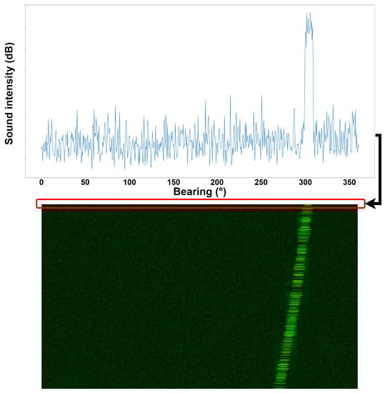
Figure 1.
Example of how the received sound signal is converted to a bearing–time record (BTR) image.
Figure 2 shows an example scenario, which depicts the underwater environment in which this BTR image is generated. Various factors, such as water temperature, seafloor topography, marine life, and water depth, can impede the acquisition of precise bearing measurements. The presence of background noise resulting from these factors exacerbates the likelihood of the target not being detected, consequently causing the bearing trajectory to appear fragmented in the BTR image, as shown in Figure 3, which presents real BTR images. The successful execution of a military operation hinges upon the acquisition of continuous and precise bearing information of enemy ships [3]. Hence, the task of predicting undetected bearing information in BTR images is required [4].
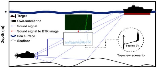
Figure 2.
Illustration of an underwater scenario wherein a BTR image is generated.
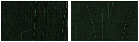
Figure 3.
Real BTR images.
In previous studies, traditional image processing methods have been utilized to extract or segment objects from SONAR images [5,6]. Although these algorithms can extract targets from noisy images, they lack the experiments to validate whether the methods can segment a continuous target object from a discrete source object. In this paper, we propose a deep-learning-based segmentation network that can extract targets as a continuous form, even from discontinuous and noisy BTR images. The network’s objective is to learn how to predict a continuous target trajectory from an input image with a discontinuous target trajectory in a supervised learning manner using noisy BTR images and their corresponding label images.
Deep-learning-based segmentation networks have been used for many practical applications, including face recognition [7,8] and detection [9,10], medical image analysis [11,12], computer vision for autonomous vehicles [13,14], etc. For image segmentation studies, convolutional neural networks (CNNs) and attention-model-based transformer networks have been the predominant methods [15,16,17,18]. However, acquiring a large training dataset for network learning can be challenging, particularly when the data contain classified military information. To address this issue and facilitate research and experimentation, we generated a synthetic BTR image dataset using the modeling and simulation (M&S) technique [19]; an example of a simulated BTR image and its corresponding label image are presented in Figure 4.
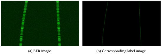
Figure 4.
An example of our synthetic BTR image dataset.
Existing segmentation models are subject to limitations when applied to the task of tracking objects in BTR images. Unlike natural images, target objects in BTR images exhibit distinct characteristics; for example, they have disjointed, elongated, and linear nature in the presence of substantial background noise. Moreover, a significant class imbalance exists between the background and target object in terms of the number of pixels. As a result, existing segmentation models, which are intended for general images, cannot provide satisfactory performance for the extraction of target trajectories from BTR images. To increase the segmentation performance, we propose a novel spatial convolutional layer in the proposed deep network, which considers the aforementioned characteristics of the target object. In addition, we introduce new loss functions for network training to address the class imbalance problem. We evaluated the performance of our proposed network against state-of-the-art models using our synthetic BTR image dataset.
The rest of this paper is organized as follows. We review related work on deep-learning-based image segmentation and commonly utilized loss functions in Section 2. Our synthetic BTR image dataset and the proposed segmentation network are presented in Section 3 and Section 4, respectively. Experimental results are presented and discussed in Section 5. Finally, concluding remarks are presented in Section 6.
2. Related Work
2.1. Semantic Image Segmentation
Semantic segmentation is a computer vision task, the objective of which is to generate a dense, pixel-wise segmentation map of the image, where each pixel is assigned to a distinct class or object. In recent years, several CNN-based deep network models have been developed for semantic segmentation that have achieved impressive results on various benchmark datasets, such as PASCAL VOC 2012 [20], Trans10K [21], ADE20K [22], and Cityscapes [23]. Among these models, DeepLab-v3+ (DLV3+) [24] and SegNeXt [25] have gained significant popularity due to their excellent performance. Specifically, DLV3+ employs the atrous (dilated) convolution technique to efficiently apply filters with a broad receptive field without increasing computational complexity. By adjusting the dilation rate, the model obtains feature maps at varying resolutions, enabling improved segmentation performance through the atrous spatial pyramid pooling (ASPP) module, which collects information at multiple scales. Furthermore, DLV3+ leverages an encoder–decoder structure with skip connections to enhance the resolution of the segmentation prediction map. SegNeXt also adopts a CNN-based backbone network with an integrated convolutional attention module, enabling efficient encoding of contextual information by prioritizing essential regions, thereby enhancing segmentation performance.
Previous studies, such as [26,27], have employed CNN-based networks for sonar image segmentation. These studies dealt with a common challenge of segmenting images with backgrounds that have significant noise. In [26], the inclusion of a deep separable residual module enabled multiscale feature extraction, leading to improved model accuracy. The dataset used in [27] contains foreground objects with long, linear shape features; the authors addressed the challenges of strong noise and class imbalance by using an architecture with skip connections and a weighted loss function. The utilization of a CNN-based spatial convolutional (SC) layer module has been shown to enhance the performance of semantic segmentation [28]. Another study [29] also utilized an SC layer in an instance segmentation model to detect transmission lines with long and linear shapes. The module effectively extracted objects with long, continuous features, such as road lanes. In addition, there are visual measurement applications related to our research field, such as that reported in [30,31], wherein CNN-based segmentation networks were used to perform width measurements of cracks on structures like buildings and roads.
In this study, we present a novel CNN-based segmentation model that builds on the DLV3+ architecture. The BTR image dataset used in our study comprises target objects that are characterized by discontinuous long and linear features similar to those in [29]. This feature complicates the segmentation task, since the objective is not only to segment the target objects but also to fill gaps in a natural and seamless manner. Moreover, the BTR image dataset presents a more intricate challenge due to the fact that the label images contain only one pixel value per row, reflecting one value per time of bearings. This situation results in a more severe class imbalance than that reported in [29]. To address this issue, we propose an extended spatial convolutional (ESC) layer module and a modified spatial convolutional (MSC) layer module that are integrated into the DLV3+ model to enhance the accuracy of target object extraction. We benchmarked the performance of our model against three state-of-the-art models—DeepLabv3+, SegNeXt, and ViT-Adapter [32]—which have demonstrated satisfactory performance on various datasets.
2.2. Loss Function
The cross-entropy (CE) loss function is commonly used to train segmentation networks. However, its effectiveness is limited when the class distribution in the dataset is imbalanced, as observed in the BTR image dataset. To overcome this type of challenge, several studies have explored alternative loss functions.
Focal loss [33] is a loss function that tackles class imbalance by reducing the loss weight assigned to correctly classified pixels. This helps prevent the loss function from being dominated by a large number of easily classified classes. Tversky loss [34] is a loss function specifically designed for medical applications, such as lesion segmentation, where recall performance is crucial. By assigning different weights to recall and precision indices, learning performance can be improved in the desired direction. Focal Tversky loss [35] combines the concepts of focal loss and Tversky loss, effectively addressing class imbalance and enabling weighted learning of recall and precision. In the BTR image segmentation task, recall performance is crucial, similar to the lesion segmentation task, due to class imbalance. In this study, we effectively address this problem by proposing a new loss function that combines Tversky loss and focal Tversky loss to increase the segmentation performance for various evaluation metrics.
3. Synthetic BTR Image Dataset
In order to create diverse scenarios for the acquisition of underwater sound signals, a variety of conditions were considered when simulating the BTR image dataset. Several aspects of the marine environment can cause discontinuity in the trajectory of target bearing information and introduce noise in the background of BTR images. To simulate these factors, we considered four specific conditions: (1) three levels of background noise (strong, moderate, and weak), (2) three levels of probability of target detection (PD) (100%, 80%, and 50%), (3) two types of bearing information (absolute bearing and relative bearing), and (4) two different patterns of target movement (constant and varying movements). As a result, our BTR dataset can encompass various warfare scenarios for both one’s own submarine and an enemy ship. Specifically, a total of 48 simulated BTR datasets can be generated for a single target motion case. Moreover, the dataset was expanded to include scenarios with dual targets. A summary of our synthetic BTR dataset is presented in Table 1, where the single and dual target scenarios include a total of 192,000 and 95,568 cases, respectively.

Table 1.
Summary of our synthetic BTR image dataset.
An example of a BTR label image and a BTR test image is presented in Figure 5, where the BTR label image contains absolute bearing information in one motion with 100% PD and no noise. To be more specific, simulated BTR images (Figure 5b) with dimensions of 1200 × 700 were generated. The horizontal axis represents bearing information ranging from −180° to 180° at an interval of 0.3° per pixel, while the vertical axis represents time information, where per second images are captured in order from top to bottom. The bit depth of a pixel is 8 bits, representing brightness values ranging from 0 to 255. It should be noted that the corresponding label images (Figure 5a) have a binary pixel value, where the target’s bearing information is represented by 255, while non-target areas have a value of 0. BTR label images have only one non-zero pixel in each row as bearing information. However, actual measurement images tend to display the target trajectory with a certain thickness, caused by several noise factors, as depicted in Figure 5b. To account for this, we simulated the trajectory of target bearing information in the horizontal direction using Gaussian modeling as follows:
where represents the values of the pixels that are generated in Figure 5b based on the bearing information of the target in Figure 5a, and corresponds to the bearing value of the target in Figure 5a and has a pixel value of 255. In order to enhance the similarity to real BTR images, where the thickness of the target trajectory varies at each time step, we simulated the thickness using a Gaussian model with a random selection of values for each time step. Therefore, pixel value of the object in Figure 5b is attenuated as deviates from the bearing position.
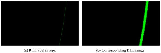
Figure 5.
An example of a synthetic BTR image pair.
To ensure that our simulated dataset covers various and detailed target motion scenarios, we assumed constant velocity motion of enemy ships at speeds of 5, 10, and 15 knots (1 knot is equivalent to 1.85 km/h), and distances from one’s own submarine were assumed to be 10 and 18 km. In real submarine warfare systems, if the one’s own submarine moves straight, it can only acquire bearing information of the target. To obtain the distance information of the enemy ship, one’s own submarine needs to alter its course. To account for this during BTR dataset generation, one’s own submarine’s path change is performed twice, with each straight motion lasting between 180 and 200 seconds, with an angular velocity change of 0.3° to 0.5° per second. The speed of one’s own submarine was set to 3, 5, and 7 knots, and the depth of one’s own submarine was assumed to be 150 m from the sea surface.
3.1. Absolute Bearing and Relative Bearing
In the context of target tracking, two types of BTR images were generated with absolute and relative bearing information. The bearing represents the 2D plane angle of the enemy ship as observed from the top view (see Figure 2). A relative bearing represents the angle relative to the heading of one’s own submarine. On the other hand, an absolute bearing represents the angle with respect to north as the 0° reference point. Two different types of bearing are illustrated in Figure 6, and the movement of one’s own submarine is reflected in (b).
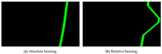
Figure 6.
An example of BTR images based on two types of bearing.
3.2. Presence of Sinusoidal Variation
To reflect diverse challenges encountered during target tracking, the BTR images were produced in two distinct formats. The first type of BTR image portrays the target’s bearing trajectory as a simplistic straight line, assuming a constant motion of the enemy ship without any deviation from its path (Figure 7a). The second type of BTR image incorporates more varying target movements in the form of sinusoidal oscillations along the vertical axis (Figure 7b).
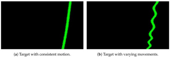
Figure 7.
An example of BTR images depending on whether or not sinusoidal variation is reflected.
3.3. Background Noise and Probability of Detection
To simulate background noise in BTR images, the additive white Gaussian noise (AWGN) function was utilized, with four noise levels applied in terms of the signal-to-noise ratio (SNR). These SNR values included 5, 10, and 15, with a no-noise scenario also considered. As the SNR decreases, the degree of noise increases. An example of a BTR image with background noise is demonstrated in Figure 8.
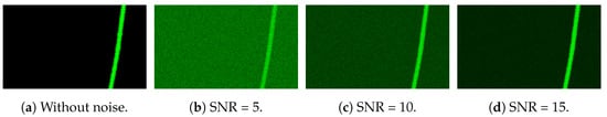
Figure 8.
BTR images with different levels of additive white Gaussian noise (AWGN) added.
The BTR dataset was designed to accommodate intermittent target measurements by incorporating three distinct probabilities of detection (PD): 50%, 80%, and 100%. The term PD refers to the likelihood of target detection per frame, with 100% indicating the availability of target bearing information across all frames. Visual representations of BTR images with different PD values are shown in Figure 9.
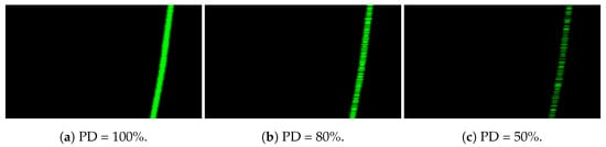
Figure 9.
BTR images with different probabilities of target detection (PD).
For learning and experimentation purposes, the BTR images without noise were excluded. Thus, nine BTR images were generated by combining three different levels of noise and three different PD values for each case, as depicted in Figure 10.
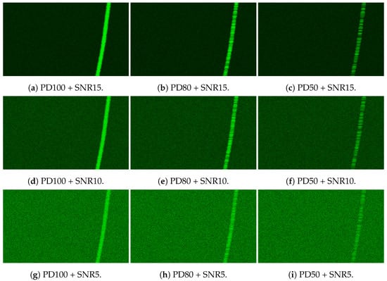
Figure 10.
A set of nine BTR images with different SNR and PD combinations.
3.4. BTR Images of Dual Targets
The BTR images presented thus far consider only a singular target, with each image singularly featuring a sole target. The setup for images containing two targets is akin to that of single-target images. Figure 11 shows a BTR image of a dual-target scenario, which was generated through the summation of individual target simulations.
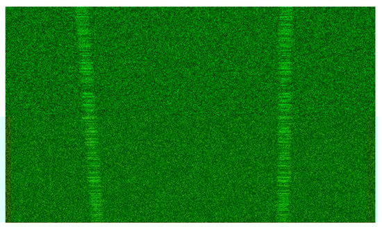
Figure 11.
A BTR image with dual targets.
3.5. Process of Generating the BTR Dataset
Based on the mentioned information, the BTR image dataset was generated using Matlab. The generation process can be summarized as follows:
- (Step 1)
- Based on the mentioned conditions, one case is determined among the cases corresponding to the motion of one’s own submarine and the enemy ship. Subsequently, for each determined case, a single label image is generated based on the bearing conditions (Section 3.1) and the presence of sinusoidal variation (Section 3.2);
- (Step 2)
- The label image obtained in the previous step is used to simulate the horizontal width according to Equation (1);
- (Step 3)
- For the PD cases described in Section 3.3, one PD value is specified to generate discontinuous bearing information;
- (Step 4)
- For the SNR cases described in Section 3.3, one SNR value is specified to simulate the background noise of the image.Combining all these steps results in the generation of one BTR image.
4. The Proposed Deep Segmentation Network
This section provides a detailed description of the proposed network architecture and novel loss functions for network training.
4.1. Network Architecture
While many deep-learning-based segmentation models, including DLV3+, are commonly trained on datasets with diverse object shapes, the BTR dataset only contains objects with elongated shapes. To handle such shapes and improve target segmentation performance, we propose the addition of an ESC layer module or an MSC layer module to the baseline DLV3+ network architecture. The overall architecture of the proposed network is shown in Figure 12 and Figure 13. Positioned between the output of the backbone network layer and the input of the ASPP layer, the ESC/MSC layer effectively extracts features pertaining to objects of elongated shape.
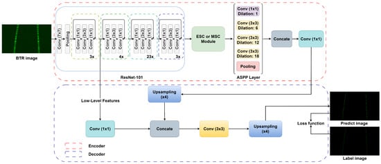
Figure 12.
The proposed deep segmentation network.
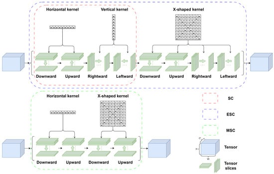
Figure 13.
The architecture of the ESC and MSC modules.
As shown in Figure 12, the input image proceeds through the initial stage of feature extraction by the ResNet-101 backbone network [36]. The resulting feature map, which is reduced in spatial size by a factor of 1/16, is subsequently fed into the MSC (or ESC) layer. The ASPP layer then employs kernels with varying scaling ratios to aid in extraction of targets with different widths per row in the BTR image. After the ASPP layer, a 1 × 1 convolution is utilized to reduce the number of channels, followed by a 4× upsampling process that aligns it with the low-level features from ResNet-101, which have also undergone a 1 × 1 convolution. Subsequently, a 3 × 3 convolution takes place, followed by a 4× upsampling operation, resulting in a segmented image with the original image resolution.
The ESC and MSC modules shown in Figure 13 can make the SC module proposed in [29] more well-suited to the distinct characteristics of BTR images. Specifically, the ESC is a module that adds additional sublayers to the existing SC layer module. In the sublayers, the convolution operation is performed four times with an X-shaped kernel, in the order of downward, upward, rightward, and leftward directions. The MSC comprises a series of downward, upward, downward, and upward sublayers with the horizontal kernel and X-shaped kernel, respectively. Each sublayer of the ESC and MSC modules maintains a tensor size consistent with both its input and output.
Through such directional convolution operations and the kernels, the ESC and MSC modules can play a role in filling the discontinuities observed in BTR images along the bearing trajectory. To be specific, the convolutional output of the downward and upward sublayers corresponding to the i-th row is added to the tensor slice of the subsequent (i + 1) row. Similarly, for the rightward and leftward sublayers, the convolutional output of the i-th column is added to the tensor slice of the (i + 1)-th column; then, the convolution operation of the (i + 1)-th column is performed. Furthermore, the use of an X-shaped kernel can help to segment target objects with diagonal directions. For the ESC module, the rightward and leftward sublayers with a vertical kernel may be effective for extracting horizontal features. However, they may result in an unnecessary summation between the target object and background noise in BTR images. Consequently, these directional sublayers in the MSC and ESC layers enable the network to effectively connect fragmented spatial features in BTR images.
In addition to the proposed ‘DLV3+ with ESC (DLV3+ESC)’ and ‘DLV3+ with MSC (DLV3 + MSC)’ networks, we also evaluated other network architectures, such as the ‘DLV3+ with SC (DLV3 + SC)’ network, which integrates the original SC layer onto the DLV3+ baseline. Our experimental results reveal that the ‘DLV3 + MSC’ network outperformed the other two networks. A comprehensive discussion of the experimental results is presented in Section 5.
4.2. New Loss Functions for Network Training
In this section, we propose novel loss functions for network training to address the severe class imbalance problem between the foreground and background regions of the BTR images. The confusion matrix shown in Table 2 is widely used for the evaluation of image segmentation models. In our BTR image dataset, true positive (TP) and false positive (FP) are employed to describe cases in which the network’s prediction correctly and incorrectly classifies a given pixel as belonging to a target-bearing object, respectively. Similarly, true negative (TN) and false negative (FN) represent cases in which the network’s prediction correctly and incorrectly assigns a given pixel to the background class, respectively.
Table 2.
Confusion matrix for the BTR dataset.
In the BTR dataset, the main goal is to minimize FNs, i.e., failure to predict actual target-bearing pixels, since there are only a few target-bearing pixels, and it is crucial to secure the accuracy of those pixels to obtain satisfying objective and subjective segmentation results. To achieve this, we propose two loss functions: modified Tversky loss (MTL), a variant of the Tversky loss [34], and modified focal Tversky loss (MFTL), a variant of focal Tversky loss [35].
Tversky loss (TL) is a powerful model for balancing the tradeoff between different classes by assigning different weights to FN and FP, which improves the overall performance of the model. It is expressed by the formula , where indicates the Tversky index as:
where p denotes the predicted value assigned to a pixel by the trained network, indicating its likelihood of belonging to the target class. It is a real number ranging between 0 and 1. Meanwhile, y represents the pixel value in the BTR label image, where a value of 0 corresponds to the background class, and a value of 1 corresponds to the target class. can be expressed in terms of TP, FP, and FN as follows:
In studies involving lesion segmentation tasks [34], it is more important to avoid failing to predict true lesions (FN) than falsely identifying normal regions as lesions (FP). Therefore, reducing FN over FP becomes the primary objective. To achieve this objective, the network can be trained to assign a higher weight to (FN) compared to the weight assigned to (FP). Since the main goal of our study is to reduce FNs, we propose the use of modified TL to further increase the segmentation performance as follows:
To effectively decrease the occurrence of FNs in the network output, we present a technique to amplify the significance of FN by squaring the value of p in the FP expression.
Focal Tversky loss (FTL) utilizes a exponent greater than 1 to allow the network to concentrate more on challenging cases during training. As an example with a value of 2, when the training is unsuccessful and TL yields a large loss value such as 0.9, the FTL output decreases by a relatively small ratio to 0.81. However, when the training is effective and TL produces a small loss value like 0.1, the FTL output decreases significantly to 0.01. As a result, FTL effectively enhances segmentation performance by increasing the relative weighting of challenging cases compared to easy cases in the loss function. It is mathematically expressed as:
Similar to MTL, the proposed MFTL is a modified version of FTL, as shown below.
5. Experimental Results and Discussion
5.1. Experimental Environment
The experiments were conducted on a hardware setup consisting of an Intel Xeon Processor with 128 GB RAM, a Windows Server operating system, and an NVIDIA Tesla V100 GPU. The network implementation was performed using Python 3.8 and PyTorch 1.7.1. The learning optimization algorithm was mini-batch stochastic gradient descent (SGD) with an initial learning rate of 0.01, and the poly learning rate policy was applied during the training process.
5.2. Datasets
Our synthetic BTR image dataset was classified into nine distinct subdatasets based on three levels of noise (SNR: 5, 10, and 15) and three different PDs (50%, 80%, and 100%). Each subdataset comprises an equal distribution of BTR images that encompass sinusoidal and non-sinusoidal, relative, and absolute bearing, as well as dual- and single-target scenarios. To evaluate the performance of the proposed network in different scenarios, the nine subdatasets were organized into three experimental datasets, key features of which are summarized in Table 3.
Table 3.
Features of the three experimental datasets.
5.2.1. PD100 + SNR15 Dataset
The first experimental dataset represents an ideal scenario of an uninterrupted target and minimal noise interference (PD = 100% and SNR = 15). We conducted experiments on this dataset to assess the performance of the proposed model under the most favorable conditions. The training dataset consisted of 19,164 images, the validation dataset comprised 300 images, and the test dataset contained 1000 images.
5.2.2. PD50 + SNR5 Dataset
The second experimental dataset represents the most challenging scenario among the simulated BTR datasets and is characterized by the highest noise level of SNR = 5 and a 50% probability of target disconnection. In contrast to the PD100 + SNR15 dataset, it poses greater difficulties for the segmentation task. The training dataset consisted of 19,164 images, the validation dataset comprised 300 images, and the test dataset contained 1000 images.
5.2.3. Nine-Case Composite Dataset
In the third experimental setting, the same number of BTR images containing all nine cases was used for training, validation, and testing to assess the overall target segmentation performance of the proposed network. The training dataset comprised 40,500 images, the validation dataset consisted of 2700 images, and the test dataset comprised 2700 images.
5.3. Evaluation Metrics
For segmentation tasks, the mean intersection over union (MIoU) is commonly used as a performance metric. However, in the context of the BTR image dataset, which comprises only two classes (background and target) with a significant class ratio imbalance, MIoU is not an appropriate metric for performance assessment. Instead, we employed four metrics: recall, precision, and scores ( = 1 and 3), hereafter denoted as score and score, respectively, which are expressed as follows.
The recall increases as the number of FN pixels decreases, while the precision increases as the number of FP pixels decreases. Given that the primary objective of this work is to enhance the detection rate of the target’s bearing by reducing FNs, the improvement in the recall metric is considered more crucial than precision. Furthermore, due to the discontinuity of target objects and their varying widths, the network occasionally produces predictions with a width larger than one, in contrast to the label image’s bearing pixel width of one. Consequently, this leads to relatively lower precision results. However, it is important to note that this phenomenon does not pose a problem in bearing detection, as the network’s predicted pixels can be effectively aggregated by taking their average values. While the score reflects an equal balance between FP and FN, the score, which assigns greater weight to recall than precision, aligns with our purpose and was therefore selected as the primary evaluation metric. Previous studies, such as [37,38], also utilized the score as the main metric.
5.4. Quantitative Evaluation
The performance of the proposed network was compared with three state-of-the-art networks:" DLV3+ [24], SegNext [25], and Vit-Adapter [32]. SegNext and Vit-Adapter were tested because they have shown high performance on various semantic segmentation datasets, and the base model, DLV3+, was also compared. To ensure a fair comparison, instead of using pretrained networks provided by the authors, test networks were trained on our BTR dataset. The two proposed networks, DLV3+ with ESC and DLV3+ with MSC, were designed to capture the spatial features associated with vertical and diagonal directions by adding a set of kernels to the existing SC layer, where these kernels are arranged in different orders within each network.
In quantitative evaluation, we focused on conducting a thorough analysis of the recall and -score metrics. Additionally, the results of precision and score are included for informative purposes to provide a comprehensive understanding of the performance characteristics. The experimental results are summarized in Table 4, where the highest scores for recall and score are highlighted in bold for each dataset. It is worth mentioning that all the results in Table 4 were obtained by training five networks with the same cross-entropy loss function.
Table 4.
Quantitative evaluation on the BTR image dataset. All test networks were trained using the cross-entropy loss function.
5.4.1. Results of Using the Cross-Entropy Loss Function
In this subsection, the experimental results of the three datasets trained by the cross-entropy loss function are analyzed.
(a) The results of the PD100 + SNR15 dataset are presented as follows. The proposed DLV3 + ESC shows the highest performance, with recall and -score metrics of 50.49% and 46.41%, respectively. When compared to the second-highest-performing model, DLV3 + SC, our approach demonstrates a significant improvement of approximately 11.53% and 9.17% in recall and score, respectively. These results validate that the introduction of new directional sublayers and the novel X-shaped kernel in the SC layer is highly advantageous for effectively extracting elongated features from BTR images. It is worth noting that the SOTA models, SegNeXt and ViT-Adapter, exhibit notably poor performances in terms of recall and score, e.g., i.e., than 20%. This can be attributed to their lack of specialized network modules designed to consider such distinctive feature characteristics.
(b) For the challenging PD50 + SNR5 dataset, SegNeXt achieved the highest recall and score. It outperformed the proposed DLV3 + SC model by a margin exceeding 5%. Notably, even SegNeXt achieved a recall rate below 10%, indicating that all tested networks encountered difficulties in accurately segmenting the target pixels. These results suggest that training the proposed network using the traditional CE loss function fails to effectively optimize its performance due to several factors, including the presence of strong noise, the presence of discontinuous targets, and the existence of class imbalance. These challenges prevent the achievement of satisfactory segmentation results during the training process.
(c) Lastly, in the case of the results obtained from the nine-case composite dataset, the proposed DLV3 + ESC network outperforms the other networks. Specifically, when compared to SegNeXt, DLV3 + ESC demonstrates noteworthy enhancements of 2.63% in recall and 4.89% in F3 score. However, it is important to note that despite these improvements, the overall performance of DLV3 + ESC remains relatively low, achieving 22% recall.
Table 5 presents the experimental results of the proposed DLV3 + MSC network when utilizing the proposed MTL or MFTL loss functions instead of the CE function. The hyperparameters of the loss function were configured as , , and . Based on the recall and -score metrics, it is evident that the overall experimental results presented in Table 5 show significant improvements compared to those in Table 4. Specifically, for the nine-case composite dataset, the recall score increases substantially to 92.28% from 21.81%.
Table 5.
Experimental results of DLV3 + MSC on the BTR image dataset when trained using the proposed loss functions.
5.4.2. DLV3 + MSC: Results of the Proposed Loss Functions
The experimental results of the three datasets trained by the proposed DLV3 + MSC network and the proposed loss functions are analyzed in this subsection.
(a) First, we present the results of the PD100 + SNR15 dataset. When comparing the performance of the DLV3 + MSC trained using MTL with that of the DLV3 + ESC trained using CE loss, notable enhancements are observed. Specifically, the DLV3 + MSC model exhibits remarkable improvements, exceeding 40% and 30% in recall and score, respectively, over the DLV3 + ESC network.
(b) For the the PD50 + SNR5 dataset, the DLV3 + MSC achieves a high recall rate of 72.38% and an score of 54.98%. As observed in Table 4, the proposed network trained with the CE loss function failed to attain satisfactory segmentation performance on this particularly demanding dataset. Therefore, the incorporation of the proposed loss function proves beneficial, as it enables the network to address the challenge of class imbalance, thereby enhancing its robustness and reliability. However, it shows relatively low performance compared to other datasets, so there is a need for further improvement in the future.
(c) As observed in the experimental results on the nine-case composite dataset, the proposed network with novel loss functions shows exceptional average segmentation performance, specifically a recall rate of 92.28% and an score of 73.28%. These results suggest that the proposed loss functions consistently surpass the performance of the CE function, providing superior enemy-tracking performance for diverse warfare scenarios.
5.5. Qualitative Evaluation
In this section, we conduct a comparative analysis of the subjective quality of the predicted images generated by the respective test networks.
5.5.1. Networks Trained Using the Cross-Entropy Loss Function
Figure 14 presents a qualitative visual quality comparison of the models trained using the CE loss function. The images were sourced from the PD100 + SNR15 and PD50 + SNR5 datasets for the dual-target scenario. The first and second rows show the test images and the corresponding label images, respectively. The label images have a single non-zero pixel per row, representing the bearing value of the target per second. In these test images, the spacing between dual targets decreases as moving down the rows, thereby posing a greater challenge for accurate target separation. Additionally, the bearing trajectories of the targets in these images demonstrate both diagonal and vertical directions. The third to seventh rows exhibit the predicted images of each network.
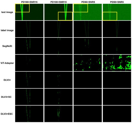
Figure 14.
Qualitative comparison among the test networks trained using CE loss. For ease of observation, the yellow boxed areas in the first row are magnified in the subsequent rows.
Upon inspection of the image predicted by SegNeXt for the PD100 + SNR15 image in the second column, it is evident that the target is not detected in the middle of the object. Additionally, in the lower parts of the image, where the distance between the two targets is short, the target bearings are not predicted separately but incorrectly predicted as one. The trend is the same in the predicted image of the PD50 + SNR5 image, with fewer target pixels correctly predicted. The predicted images in the second column also have a diagonal break in the object. The worst result is observed in the PD50 + SNR5 image in the fourth column, which is the most challenging scenario, where SegNeXt almost failed to segment the target trajectory.
The Vit-Adapter network generally exhibits notably inadequate qualitative performance across all predicted images. When examining the predicted images in the first and second columns, only a few pixels near the top of the images demonstrate successful segmentation. Even worse, the target prediction fails completely for the PD50 + SNR5 test images in the third and fourth columns.
Regarding the PD100 + SNR15 outcomes obtained from DLV3+, similar to SegNeXt, noticeable discontinuities are observed in the target prediction. Additionally, in the lower parts of the images, the network exhibits a failure to accurately predict the targets. As for the PD50 + SNR5 results, a majority of the pixels are classified as background, indicating a significant shortfall in target identification. On the other hand, for DLV3 + SC, there is some improvement in target prediction in the lower parts of the images in the third and fourth models compared to DLV3+.
The proposed DLV3 + ESC network, as depicted in the predicted image in the second column, demonstrates a higher target detection rate compared to previous results. This improvement can be attributed to the integration of the ESC layer module, which incorporates a diagonal kernel, enabling consideration of the directionality of the spatial features. However, when faced with the demanding PD50 + SNR5 dataset, the third and fourth figures clearly indicate that a substantial number of targets remain undetected.
In summary, for the majority of networks trained with the CE loss function on the PD100 + SNR15 dataset, less than half of the bearing target segmentation results are shown. Additionally, on the more challenging PD50 + SNR5 dataset, almost no segmentation is achieved. Therefore, further improvements are imperative for the successful application of these models to military SONAR systems.
5.5.2. DLV3 + MSC Trained Using the Proposed Loss Function
The seventh and eighth rows of Figure 15 represent the segmentation results generated after training the proposed DLV3 + MSC using the MTL and MFTL loss functions. Rows 3 to 6 in the figure depict the segmentation results of the comparative models trained using the CE loss function. Overall, a noticeable enhancement in the target detection rate is observed in the results of the proposed DLV3 + MSC using the MTL and MFTL loss functions when compared to the predicted images in the comparative models.
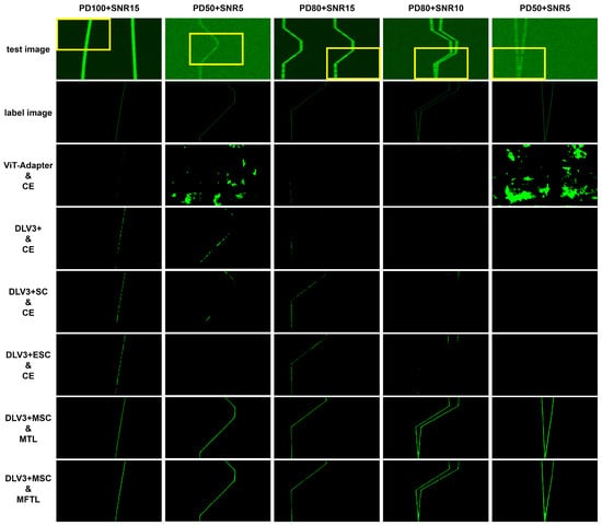
Figure 15.
Predicted BTR images obtained from the DLV3 + MSC trained using the proposed loss functions and the comparative models trained using the CE loss function. For ease of observation, the yellow boxed areas in the first row are magnified in the subsequent rows.
When comparing the results of the first and third columns, which were tested on images with low noise and high PD, the DLV3+ based models show a certain degree of target segmentation, but a considerable amount of fragmented areas are also observed. In contrast, the Vit-Adapter model exhibits lower segmentation results. However, it is evident that the results of the proposed DLV3 + MSC using the MTL and MFTL loss functions show significantly fewer discontinuous regions.
When examining the results of the second, fourth, and fifth columns, which were tested on images with relatively stronger noise and lower PD, it is evident that the DLV3+-based models struggled to effectively perform segmentation. Additionally, the Vit-Adapter model shows incorrect predictions in the second and fifth columns. In contrast, the results of the proposed DLV3 + MSC using the MTL and MFTL loss functions demonstrate robust segmentation, even in challenging images.
Finally, to compare the performance of MTL and MFTL with the proposed DLV3 + MSC model, we examine the segmentation results in the fifth column. It is noted that the MTL-based outcome demonstrates a slightly refined depiction where the two targets intersect. However, except for this specific area, discerning any significant difference between the use of the two functions is difficult. Since both the proposed loss functions aim to minimize false negatives, the overall target tracking rate is high. Nevertheless, in comparison to the label image presented in the second row, the predicted targets appear slightly thicker than the actual target pixels, and there are also some areas where certain pixels are not accurately predicted. Nonetheless, the image, as a whole, exhibits favorable target prediction capabilities for both vertically and diagonally oriented objects. Additionally, the results in the fourth and fifth columns shown that even when two targets are adjacent with strong background noise, the outcomes remain precise.
5.6. Ablation Study
In this section, we present a comparison of the MTL and TL loss functions using the same model, as well as a comparison between the DLV3 + ESC and DLV3 + MSC models when employing the proposed MTL loss function. These evaluations were carried out using the PD100 + SNR15 and PD50 + SNR5 datasets.
Table 6 presents the results obtained using the same MTL loss function. In the case of the PD100 + SNR15 dataset, it is evident that DLV3 + MSC exhibits superior performance across all metrics. For the PD50 + SNR5 dataset, DLV3 + ESC displays a higher recall metric. However, when comparing two networks based on the score, which reflects precision, DLV3 + MSC outperforms DLV3 + ESC by a notable margin of approximately 30%.
Table 6.
Performance comparison between DLV3 + ESC and DLV3 + MSC on the PD100 + SNR15 and PD50 + SNR5 datasets.
Table 7 shows a performance comparison between the original TL function and the proposed MTL function. In both datasets, there is an improvement of over 3% in the recall metric, while the score demonstrates an enhancement of approximately 3%. The score, which reflects recall and precision in the same ratio, did not decrease. Based on these results, we can conclude that the proposed loss function is successful in reducing FN and increasing the recall metric.
Table 7.
Performance comparison of using the MTL or TL for network training on the PD100 + SNR15 and PD50 + SNR5 datasets.
6. Conclusions
In this paper, we propose an efficient deep segmentation network designed to enhance the extraction of target bearing information acquired from challenging underwater environments. To facilitate the development of the proposed network and performance evaluation, we generated the synthetic BTR image dataset by simulating various factors. including underwater noise, target detection probability, target movements, etc. The proposed network architecture incorporates an MSC or ESC module, which effectively captures spatial features of elongated target trajectories. Moreover, to address the class imbalance problem inherent in traditional CE loss functions, we introduce novel loss functions: MTL and MFTL. The experimental results demonstrate that the proposed DLV3 + MSC network trained with the MTL outperformed the existing state-of-the-art segmentation networks, achieving improvement of up to 92.28% and 73.28% for recall and score, respectively. Future research will focus on further enhancing segmentation performance for the challenging PD50 + SNR5 dataset by devising a more suitable network configuration. We believe that the implementation of our deep network in existing SONAR systems has significant potential with respect to the automation of the operation military underwater warfare systems.
Author Contributions
Conceptualization, W.S., D.-S.K. and H.K.; methodology, W.S. and H.K.; software, W.S. and H.K.; validation, W.S.; resources, D.-S.K. and H.K.; data curation, W.S. and D.-S.K.; writing—original draft preparation, W.S.; writing—review and editing, H.K.; visualization, W.S. and H.K.; supervision, H.K.; project administration, D.-S.K. and H.K.; funding acquisition, D.-S.K. and H.K. All authors have read and agreed to the published version of the manuscript.
Funding
This work was supported by a Korean Research Institute for defense Technology planning and advancement (KRIT) grant funded by the Korean Government Defense Acquisition Program Administration (No. KRIT-CT-22-023-01, Deep Learning Technology for Detection & Target Tracking in low SNR, 2023).
Institutional Review Board Statement
Not applicable.
Informed Consent Statement
Not applicable.
Data Availability Statement
Data sharing is not applicable to this article.
Conflicts of Interest
The authors declare no conflict of interest.
References
- Maranda, B.H. Passive Sonar. In Handbook of Signal Processing in Acoustics; Springer: New York, NY, USA, 2008; pp. 1757–1781. [Google Scholar] [CrossRef]
- Nardone, S.; Graham, M. A closed-form solution to bearings-only target motion analysis. IEEE J. Ocean. Eng. 1997, 22, 168–178. [Google Scholar] [CrossRef]
- Northardt, T.; Nardone, S.C. Track-Before-Detect Bearings-Only Localization Performance in Complex Passive Sonar Scenarios: A Case Study. IEEE J. Ocean. Eng. 2019, 44, 482–491. [Google Scholar] [CrossRef]
- Xiong, Z.; Xu, K.; Chen, Y.; Li, G.; Wan, J. Research on multi-target bearings-only tracking method based on passive sonar systems. In Proceedings of the 2017 IEEE 2nd Advanced Information Technology, Electronic and Automation Control Conference (IAEAC), Chongqing, China, 25–26 March 2017. [Google Scholar] [CrossRef]
- Celik, T.; Tjahjadi, T. A Novel Method for Sidescan Sonar Image Segmentation. IEEE J. Ocean. Eng. 2011, 36, 186–194. [Google Scholar] [CrossRef]
- Anitha, U.; Malarkkan, S.; Premalatha, J.; Prince, P.G.K. Study of Object Detection in Sonar Image using Image Segmentation and Edge Detection Methods. Indian J. Sci. Technol. 2016, 9, 482–491. [Google Scholar] [CrossRef][Green Version]
- Parkhi, O.M.; Vedaldi, A.; Zisserman, A. Deep Face Recognition. In Proceedings of the British Machine Vision Conference 2015, Swansea, UK, 7–10 September 2015; British Machine Vision Association: Aberdeen, UK, 2015. [Google Scholar]
- Alansari, M.; Hay, O.A.; Javed, S.; Shoufan, A.; Zweiri, Y.; Werghi, N. GhostFaceNets: Lightweight Face Recognition Model From Cheap Operations. IEEE Access 2023, 11, 35429–35446. [Google Scholar] [CrossRef]
- Luu, K.; Zhu, C.; Bhagavatula, C.; Le, T.H.N.; Savvides, M. A Deep Learning Approach to Joint Face Detection and Segmentation. In Advances in Face Detection and Facial Image Analysis; Springer International Publishing: Cham, Switzerland, 2016; pp. 1–12. [Google Scholar] [CrossRef]
- Wang, W.; Dai, J.; Chen, Z.; Huang, Z.; Li, Z.; Zhu, X.; Hu, X.; Lu, T.; Lu, L.; Li, H.; et al. InternImage: Exploring Large-Scale Vision Foundation Models With Deformable Convolutions. In Proceedings of the IEEE/CVF Conference on Computer Vision and Pattern Recognition (CVPR), Vancouver, BC, Canada, 18–22 June 2023; pp. 14408–14419. [Google Scholar]
- Milletari, F.; Navab, N.; Ahmadi, S.A. V-Net: Fully Convolutional Neural Networks for Volumetric Medical Image Segmentation. In Proceedings of the 2016 Fourth International Conference on 3D Vision (3DV), Stanford, CA, USA, 25–28 October 2016. [Google Scholar] [CrossRef]
- Ronneberger, O.; Fischer, P.; Brox, T. U-Net: Convolutional Networks for Biomedical Image Segmentation. In Lecture Notes in Computer Science; Springer International Publishing: Cham, Switzerland, 2015; pp. 234–241. [Google Scholar] [CrossRef]
- Chen, B.; Gong, C.; Yang, J. Importance-Aware Semantic Segmentation for Autonomous Vehicles. IEEE Trans. Intell. Transp. Syst. 2019, 20, 137–148. [Google Scholar] [CrossRef]
- Janai, J.; Güney, F.; Behl, A.; Geiger, A. Computer Vision for Autonomous Vehicles: Problems, Datasets and State of the Art; Now Publishers: Boston, MA, USA, 2020. [Google Scholar] [CrossRef]
- Kim, Y.; Kim, S.; Kim, T.; Kim, C. CNN-Based Semantic Segmentation Using Level Set Loss. In Proceedings of the 2019 IEEE Winter Conference on Applications of Computer Vision (WACV), Waikoloa Village, HI, USA, 7–11 January 2019. [Google Scholar] [CrossRef]
- Deng, L.; Yang, M.; Qian, Y.; Wang, C.; Wang, B. CNN based semantic segmentation for urban traffic scenes using fisheye camera. In Proceedings of the 2017 IEEE Intelligent Vehicles Symposium (IV), Los Angeles, CA, USA, 11–14 June 2017. [Google Scholar] [CrossRef]
- Wang, L.; Li, R.; Duan, C.; Zhang, C.; Meng, X.; Fang, S. A Novel Transformer Based Semantic Segmentation Scheme for Fine-Resolution Remote Sensing Images. IEEE Geosci. Remote. Sens. Lett. 2022, 19, 6506105. [Google Scholar] [CrossRef]
- Strudel, R.; Garcia, R.; Laptev, I.; Schmid, C. Segmenter: Transformer for Semantic Segmentation. In Proceedings of the 2021 IEEE/CVF International Conference on Computer Vision (ICCV), Montreal, QC, Canada, 11–17 October 2021. [Google Scholar] [CrossRef]
- Etter, P.C. Underwater Acoustic Modeling and Simulation; CRC Press: Boca Raton, FL, USA, 2018. [Google Scholar] [CrossRef]
- Everingham, M.; Gool, L.V.; Williams, C.K.I.; Winn, J.; Zisserman, A. The Pascal Visual Object Classes (VOC) Challenge. Int. J. Comput. Vis. 2009, 88, 303–338. [Google Scholar] [CrossRef]
- Xie, E.; Wang, W.; Wang, W.; Ding, M.; Shen, C.; Luo, P. Segmenting Transparent Objects in the Wild. In Computer Vision—ECCV 2020; Springer International Publishing: Cham, Switzerland, 2020; pp. 696–711. [Google Scholar] [CrossRef]
- Zhou, B.; Zhao, H.; Puig, X.; Fidler, S.; Barriuso, A.; Torralba, A. Scene Parsing through ADE20K Dataset. In Proceedings of the 2017 IEEE Conference on Computer Vision and Pattern Recognition (CVPR), Honolulu, HI, USA, 21–26 July 2017. [Google Scholar] [CrossRef]
- Cordts, M.; Omran, M.; Ramos, S.; Rehfeld, T.; Enzweiler, M.; Benenson, R.; Franke, U.; Roth, S.; Schiele, B. The Cityscapes Dataset for Semantic Urban Scene Understanding. In Proceedings of the 2016 IEEE Conference on Computer Vision and Pattern Recognition (CVPR), Las Vegas, NV, USA, 26 June–1 July 2016. [Google Scholar] [CrossRef]
- Chen, L.C.; Zhu, Y.; Papandreou, G.; Schroff, F.; Adam, H. Encoder-Decoder with Atrous Separable Convolution for Semantic Image Segmentation. In Computer Vision—ECCV 2018; Springer International Publishing: Cham, Switzerland, 2018; pp. 833–851. [Google Scholar] [CrossRef]
- Guo, M.H.; Lu, C.Z.; Hou, Q.; Liu, Z.; Cheng, M.M.; Hu, S.M. SegNeXt: Rethinking Convolutional Attention Design for Semantic Segmentation. arXiv 2022, arXiv:2209.08575. [Google Scholar] [CrossRef]
- Wang, Z.; Guo, J.; Huang, W.; Zhang, S. Side-Scan Sonar Image Segmentation Based on Multi-Channel Fusion Convolution Neural Networks. IEEE Sens. J. 2022, 22, 5911–5928. [Google Scholar] [CrossRef]
- Wu, M.; Wang, Q.; Rigall, E.; Li, K.; Zhu, W.; He, B.; Yan, T. ECNet: Efficient Convolutional Networks for Side Scan Sonar Image Segmentation. Sensors 2019, 19, 2009. [Google Scholar] [CrossRef] [PubMed]
- Pan, X.; Shi, J.; Luo, P.; Wang, X.; Tang, X. Spatial as Deep: Spatial CNN for Traffic Scene Understanding. In Proceedings of the Thirty-Second AAAI Conference on Artificial Intelligence (AAAI-2018), Hilton New Orleans Riverside, LA, USA, 2–7 February 2018. [Google Scholar] [CrossRef]
- Li, B.; Chen, C.; Dong, S.; Qiao, J. Transmission line detection in aerial images: An instance segmentation approach based on multitask neural networks. Signal Process. Image Commun. 2021, 96, 116278. [Google Scholar] [CrossRef]
- Tang, Y.; Huang, Z.; Chen, Z.; Chen, M.; Zhou, H.; Zhang, H.; Sun, J. Novel visual crack width measurement based on backbone double-scale features for improved detection automation. Eng. Struct. 2023, 274, 115158. [Google Scholar] [CrossRef]
- Lee, J.S.; Hwang, S.H.; Choi, I.Y.; Choi, Y. Estimation of crack width based on shape-sensitive kernels and semantic segmentation. Struct. Control. Health Monit. 2020, 27, e2504. Available online: http://xxx.lanl.gov/abs/https://onlinelibrary.wiley.com/doi/pdf/10.1002/stc.2504 (accessed on 5 March 2023). [CrossRef]
- Chen, Z.; Duan, Y.; Wang, W.; He, J.; Lu, T.; Dai, J.; Qiao, Y. Vision Transformer Adapter for Dense Predictions. arXiv 2023, arXiv:2205.08534. [Google Scholar] [CrossRef]
- Lin, T.Y.; Goyal, P.; Girshick, R.; He, K.; Dollar, P. Focal Loss for Dense Object Detection. In Proceedings of the 2017 IEEE International Conference on Computer Vision (ICCV), Venice, Italy, 22–29 October 2017. [Google Scholar] [CrossRef]
- Salehi, S.S.M.; Erdogmus, D.; Gholipour, A. Tversky Loss Function for Image Segmentation Using 3D Fully Convolutional Deep Networks. In Machine Learning in Medical Imaging; Springer International Publishing: Cham, Switzerland, 2017; pp. 379–387. [Google Scholar] [CrossRef]
- Abraham, N.; Khan, N.M. A Novel Focal Tversky Loss Function With Improved Attention U-Net for Lesion Segmentation. In Proceedings of the 2019 IEEE 16th International Symposium on Biomedical Imaging (ISBI 2019), Venice, Italy, 8–11 April 2019. [Google Scholar] [CrossRef]
- He, K.; Zhang, X.; Ren, S.; Sun, J. Deep Residual Learning for Image Recognition. In Proceedings of the 2016 IEEE Conference on Computer Vision and Pattern Recognition (CVPR), Las Vegas, NV, USA, 26 June–1 July 2016. [Google Scholar] [CrossRef]
- Yang, R.; He, L.; Hu, X.; Zhang, B. Research on Industrial Control Network Security Based on Automatic Machine Learning. In Proceedings of the 2021 6th International Conference on Intelligent Informatics and Biomedical Sciences (ICIIBMS), Oita, Japan, 25–27 November 2021. [Google Scholar] [CrossRef]
- Straat, M.; Koster, K.; Goet, N.; Bunte, K. An Industry 4.0 example: Real-time quality control for steel-based mass production using Machine Learning on non-invasive sensor data. In Proceedings of the 2022 International Joint Conference on Neural Networks (IJCNN), Padua, Italy, 18–23 July 2022. [Google Scholar] [CrossRef]


Disclaimer/Publisher’s Note: The statements, opinions and data contained in all publications are solely those of the individual author(s) and contributor(s) and not of MDPI and/or the editor(s). MDPI and/or the editor(s) disclaim responsibility for any injury to people or property resulting from any ideas, methods, instructions or products referred to in the content. |
© 2023 by the authors. Licensee MDPI, Basel, Switzerland. This article is an open access article distributed under the terms and conditions of the Creative Commons Attribution (CC BY) license (https://creativecommons.org/licenses/by/4.0/).