Article

Construction of a Real-Time Forecast Model for Coastal Engineering and Processes Nested in a Basin Scale Model

Department of Ocean Engineering and Marine Sciences, Florida Institute of Technology, 150 W University Blvd, Melbourne, FL 32901, USA
*
Author to whom correspondence should be addressed.
J. Mar. Sci. Eng. 2023, 11(7), 1263; https://doi.org/10.3390/jmse11071263
Submission received: 25 April 2023 / Revised: 9 June 2023 / Accepted: 16 June 2023 / Published: 21 June 2023
(This article belongs to the Section Coastal Engineering)

Abstract

:
A numerical model was developed using Delft3D to simulate the circulation dynamics in Port Everglades, FL, and the adjacent coastal area. The model was nested within the HYCOM (Hybrid Coordinate Ocean Model), while meteorological data were obtained from the NARR (North American Regional Reanalysis) model. To evaluate the model, model outputs were compared with observed data from the NOAA. Calibration experiments were conducted on the model parameters, including the bottom friction, wind forcings, and vertical layer specification. These experiments revealed that implementing a 10-layer model slightly improved the vertical stratification, while the utilization of 2-D wind data resulted in more pronounced surface layer characteristics in temperature and velocity profiles and employing moderate values of the Chezy coefficient produced optimal outcomes for the bottom roughness parameter. The model demonstrated satisfactory performance across major parameters, including water level, salinity, temperature, and currents. A real-time forecast system has been constructed with this nested model, providing up to 3-day forecasts that are updated daily. To facilitate automated forecasting without manual intervention, an automation system has been developed using a combination of bash, MATLAB, and Python scripts. This study provides a comprehensive documentation of the concepts and detailed methods involved in developing a real-time forecast model for estuarine and coastal regions.

1. Introduction

The numerical modeling of estuarine and coastal hydrodynamics provides a quantitative and mechanistic understanding of critical hydrodynamic processes and is a powerful tool to predict the water movement and spatial–temporal variability of key water properties, all of which are important in marine system studies such as water quality and ecosystem dynamics. Thus, numerical modeling along with field measurement data offers comprehensive insights into estuarine dynamics. Hydrodynamic modeling forms the basis of the study of morphology, waves, sediment transport, and water quality. The principal drivers for hydrodynamics in shallow estuarine or coastal systems include tides, non-tidal sea level variations, river discharges, and meteorological forcings.
High-resolution coastal modeling has become widely used as a tool for coastal management systems. The coastal ocean conditions are also influenced by processes acting on large scales, such as the Gulf Stream. Due to their coarse resolution, global forecast models cannot resolve phenomena that require higher spatial resolutions. Down-scaling from global models could help better estimate regional features than lower resolution coarse mesh models. Therefore, nesting and down-scaling global models on to higher resolution coastal models could be a useful method to resolve coastal hydrodynamics. Developing structured grid models and nesting in large-scale models is a pragmatic approach to the problem of resolving wide-ranging spatial and temporal scales of motion [1,2,3,4]. This method involves assigning data from a coarse-resolution global model to a higher resolution model that has a smaller region of interest.
Nesting coastal models into basin-scale models combined with the assimilation of observation data will lead to improved model performance at all length scales [5,6]. Nesting a coastal model into a global ocean model such as the HYCOM could simulate the effects of the Gulf Stream by incorporating data from this large-scale model. The Gulf Stream plays a significant role on the East Coast of Florida. There is a direct correlation between sea level oscillations and Gulf Stream flow variability. In the longer term, sea level increases along East Coast in recent times could be attributed to a slowdown of the Gulf Stream [7].
Assigning open boundary conditions to coastal models is especially important, as these forced boundary conditions determine the quality of the results. The circulation in the coastal region has distinct dynamics compared to the deep ocean due to its shallowness, strong tidal influences, the neighboring coast, flow convergence and divergence due to the coast, stratification, and river outflows [8]. In coastal regions, the bottom-drag force influences are more significant than in the deep ocean; flow convergence and divergence cause surges, while horizontal density gradients cause buoyance-driven flow. To reduce the computational efforts, the model area is limited to a certain scale depending on the area of interest. The model boundary conditions are of two types—open boundary and closed boundary. To represent the influence of the area outside of model domain, which is not being modeled, open boundary conditions are prescribed. Flow and transport boundary conditions are specified at the open boundary.

2. Methods

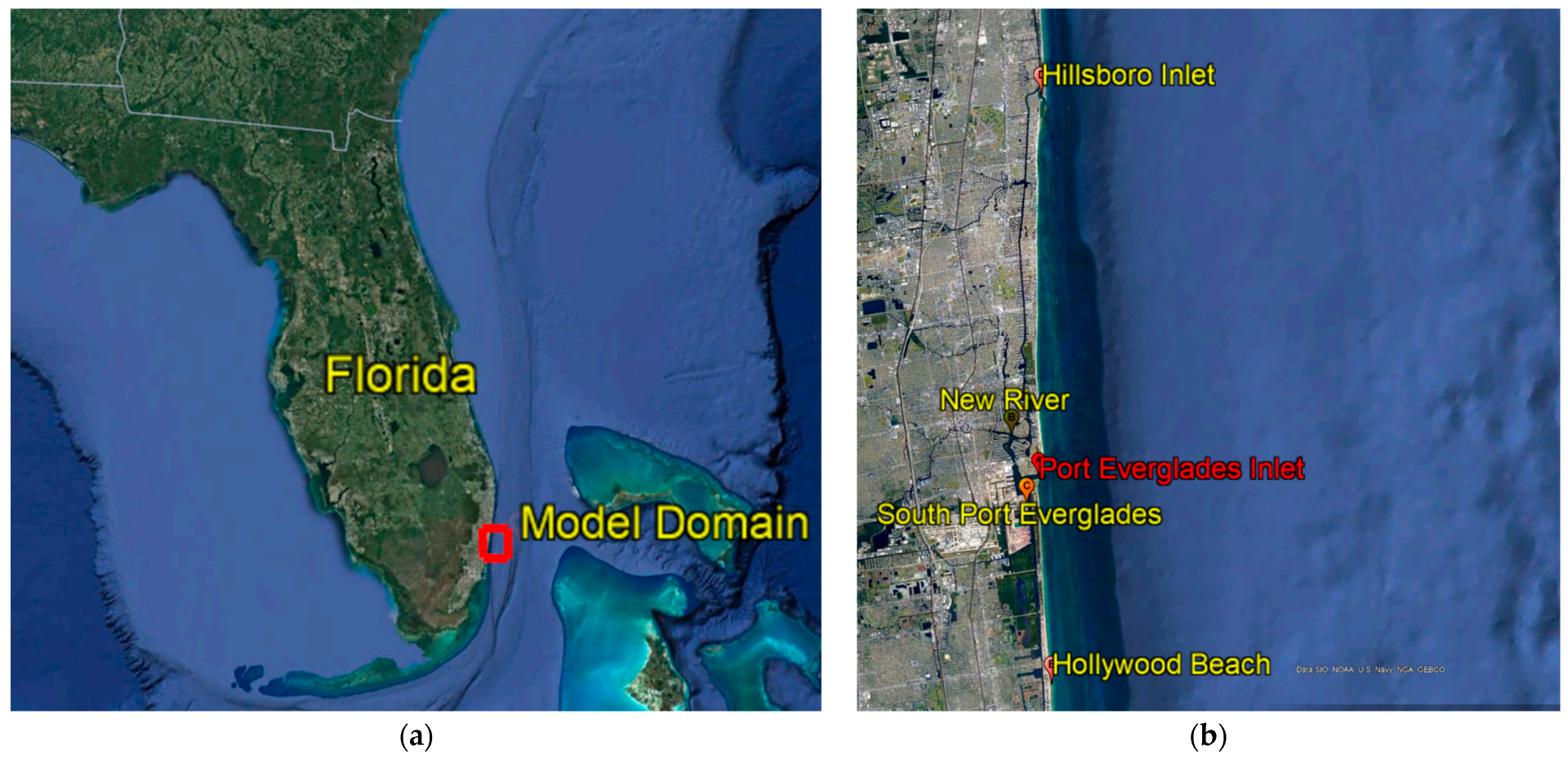
A numerical model was developed using Delft3D, an open-source, three-dimensional, finite-difference-based modeling system. The model computational grid represents a portion of the southeast Florida coast (Figure 1), from the Hillsboro Inlet to the South Lake in Hollywood Beach.

2.1. Delft3D

Delft3D is a three-dimensional computation software suite for coastal, river, and estuarine areas [9]. The Delft3D model has a modular structure including hydrodynamics (Delft3D-Flow), surface wave (Delft3D-Wave), morphology (Delft3D-Mor), and water quality (Delft3D-WAQ) aspects. In this study, the modeling and analysis were conducted solely using the Delft3D-Flow module. The model can simulate both two-dimensional and three-dimensional non-steady flow and transport phenomena driven by river discharges and tidal and meteorological forcing. The flow model can be used to predict the flow in shallow coastal areas, estuaries, lagoons, rivers, and lakes. The Delft3D-Flow module solves unsteady 2-D (depth-averaged) or 3-D shallow water equations. These equations consist of the continuity equation, the horizontal equations of motions, and the transport equations for conservative constituents [9].
Figure 1. Study area: (a) model domain (red rectangular box); (b) zoomed-in model domain in Port Everglades [10].
Jmse 11 01263 g001

2.2. Study Area

Port Everglades, Florida is located in Fort Lauderdale, about 37 km north of Miami and 77 km south of West Palm Beach, Florida. It is one of Florida’s deepest ports, covering 448 acres of submerged land and 1742 acres of upland area (Figure 1).
The tidal patterns in Port Everglades follow a semi-diurnal cycle, with the M2 tidal constituent being the most prominent. The salinity variations within the harbor of Port Everglades are influenced by several factors, including tidal flow through the inlet, rainfall, freshwater discharge, and evaporation. Furthermore, the salinity changes exhibit seasonal fluctuations, with a decrease observed during the summer months primarily due to heavy rainfall in the region.
In Port Everglades, there are various types of currents present, including littoral currents, tidal currents, and currents due to the Gulf Stream. Tidal currents are formed during ebb and flood tides and are strong in the inlet entrance both inside and outside of the jetties. The proximity of Port Everglades to the Gulf Stream results in strong currents in the offshore region.

2.3. Model Grid

The model used a curvilinear orthogonal grid with grid sizes ranging from 9 m in the river and inlets to 385 m in the coastal area (Figure 2) and had five sigma layers in the vertical direction. A spherical coordinate system was utilized in the development of the model grid. The grid was designed to represent the complex coastline, particularly the two inlets (Port Everglades inlet and Hillsboro Inlet) and harbor. The grid represents the coastline from Hillsboro Inlet to South Lake in Hollywood Beach (Figure 1).

2.4. Data Sources

The data were collected from various sources as listed in Table 1.

2.5. Topography

The topography of the current model was based on topographic data downloaded from the NOAA coastal digital elevation model [11]. The downloaded topographic data (Figure 3) were processed to construct the topography for the model domain, as depicted in Figure 2a,b.

2.6. Vertical Layer Distribution

The vertical sigma coordinates consist of 5 layers along the entire domain. These layers are distributed under a parabolic profile, extending from the thinner layer at the bottom to the thicker layer at the surface. Another model set up includes 10 sigma layers.
The numerical model developed in this study utilizes the k-epsilon turbulence formulation to simulate the vertical turbulent eddy viscosity and the vertical turbulent eddy diffusivity. The applied numerical scheme in this modeling is the alternating direction implicit (ADI) scheme [12,13,14].

2.7. Bottom Roughness

Bottom friction is specified in the boundary conditions (Equations (A3) and (A4) in Appendix A) for the momentum equations. The bottom friction is approximated by a quadratic friction law (Equation (A5)). The bottom roughness is defined under the Chezy formulation (Equation (A6)). It has a uniform roughness along the entire domain. Chezy’s U and V are two of the main parameters used to calibrate the hydrodynamics in the model. The default value for Chezy’s coefficient is 65. Various uniform values for Chezy’s coefficient (55, 65, 80, and 100) were tested during the calibration process and ultimately a Chezy coefficient equal to 55 [m1/2/s] was adopted due to its superior performance over other values.

2.8. Flow Boundary Conditions

Small errors in water levels can influence large physical areas. Therefore, placing open boundaries as far as possible from the area of interest is a strategy used to minimize the influence of errors in water level data. Weakly reflective boundary conditions need to be specified at the open boundaries so that outgoing waves from the model do not reflect at the boundary, causing disturbance in the model domain. Weakly reflective boundaries were obtained by specifying a reflection coefficient [15,16]. The reflection coefficient, denoted as alpha (Equations (A1) and (A2)), is set to 0, indicating a weakly reflective boundary.
The available types of flow boundary conditions for coastal and estuarine models include water level, velocity, water level gradient, discharge, and Riemann conditions. In this study, water level boundary conditions were applied to the model. The water level data for the boundary nodes were obtained from the HYCOM [17] and applied to the model using a nesting method. The water level data were applied to the seaward open boundary as well as the cross-shore open boundaries.
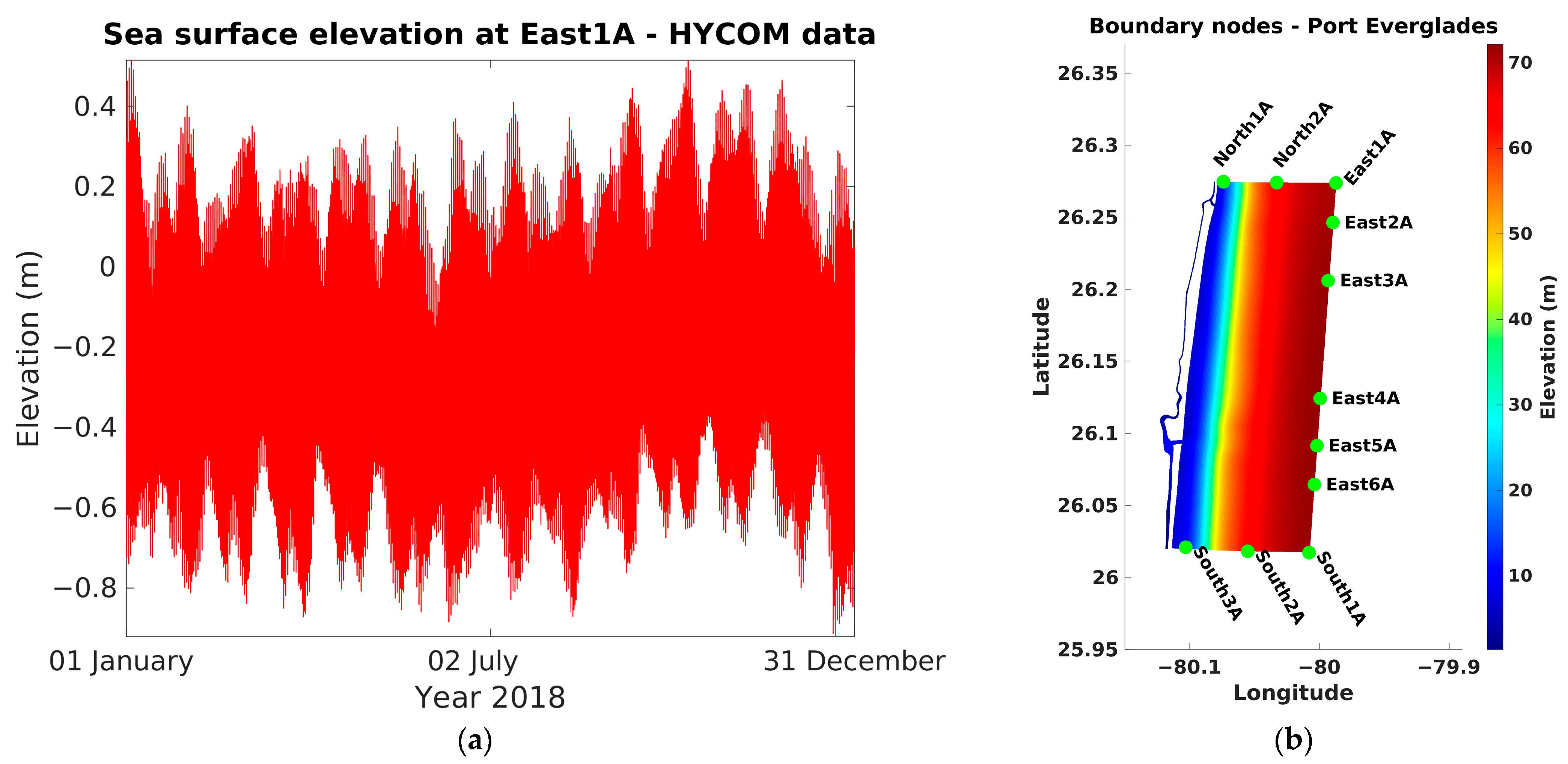
Eleven boundary nodes were selected along the north, east, and south open boundaries, including North1A, North2A, East1A, East2A, East3A, East4A, East5A, East6A, South1A, South2A, and South3A (Figure 4b). Each of these eleven boundary nodes was assigned a water level time series derived from the HYCOM. As an example of 11 time series data, Figure 4a illustrates the water level boundary conditions specifically for the East1A node.

2.9. Transport Boundary Conditions

The advection–diffusion equation represents the transport of dissolved substances such as salt, sediment, and heat. The shallow water equation has two solutions—steady-state and transient. The boundary conditions and forcing resolve the steady-state solution, whereas the transient solution is related to deviation between the initial conditions and the steady-state solution, reflection at the open boundaries, and dissipation [9]. Model boundaries were defined at locations where the grid lines were perpendicular to the flow. The inflow concentrations were specified, while allowing the concentration to be free in the outflow. Advection is the dominant horizontal transport of dissolved substances in rivers, estuaries, and coastal seas, whereas horizontal diffusion is of secondary importance. The inflow (flood) concentrations were specified while keeping the outflow (ebb) concentrations free.
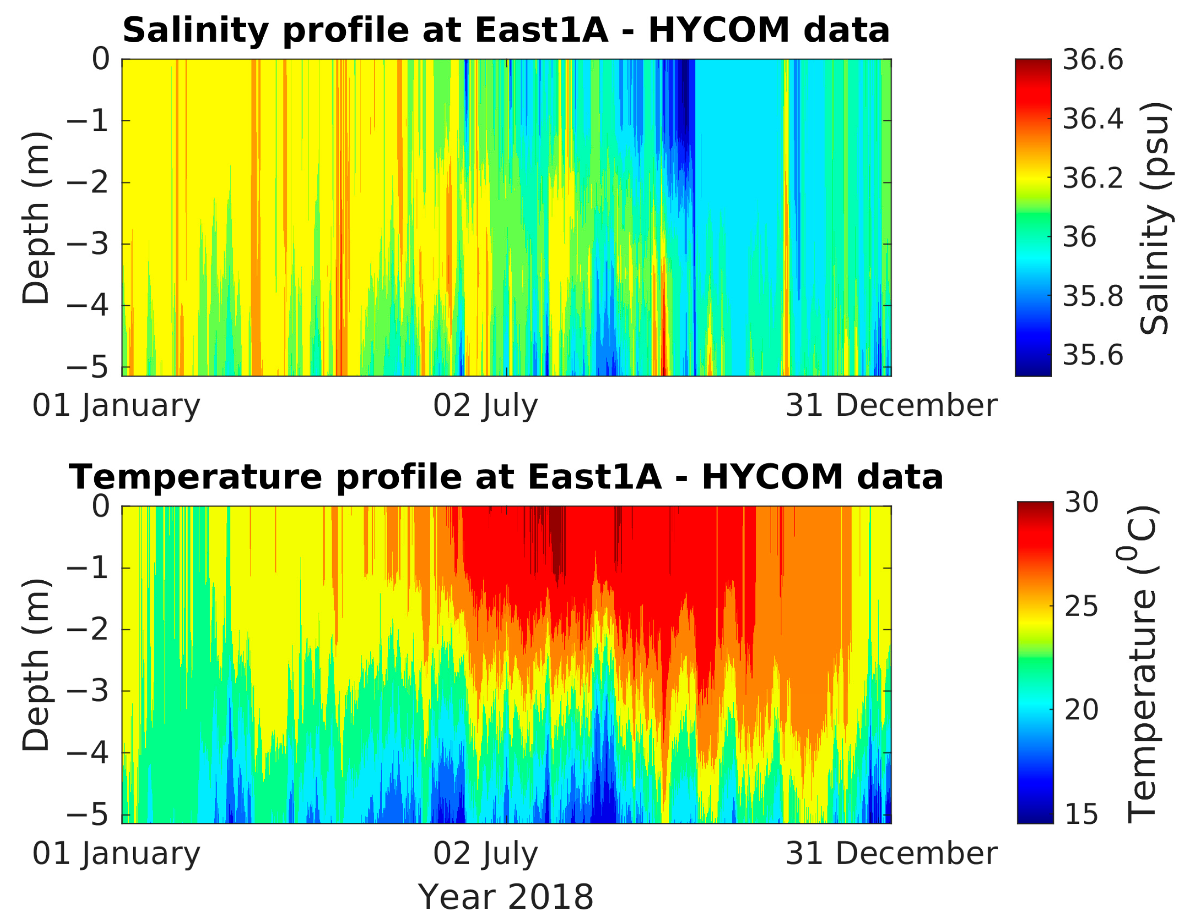
In this study, salinity and temperature were used as the transport boundary conditions. These conditions were specified in 3-D profiles consisting of 5 vertical layers. The salinity and temperature data were derived from the HYCOM [17] and applied to the model using a nesting method. Eleven 3-D profiles of salinity and temperature were assigned to each of the eleven nodes along the north, east, and south open boundaries (Figure 4b). As an illustrative example of the eleven 3D profiles of salinity and temperature, Figure 5 depicts the salinity and temperature profile at the East1A node.

2.10. Meteorological Forcing

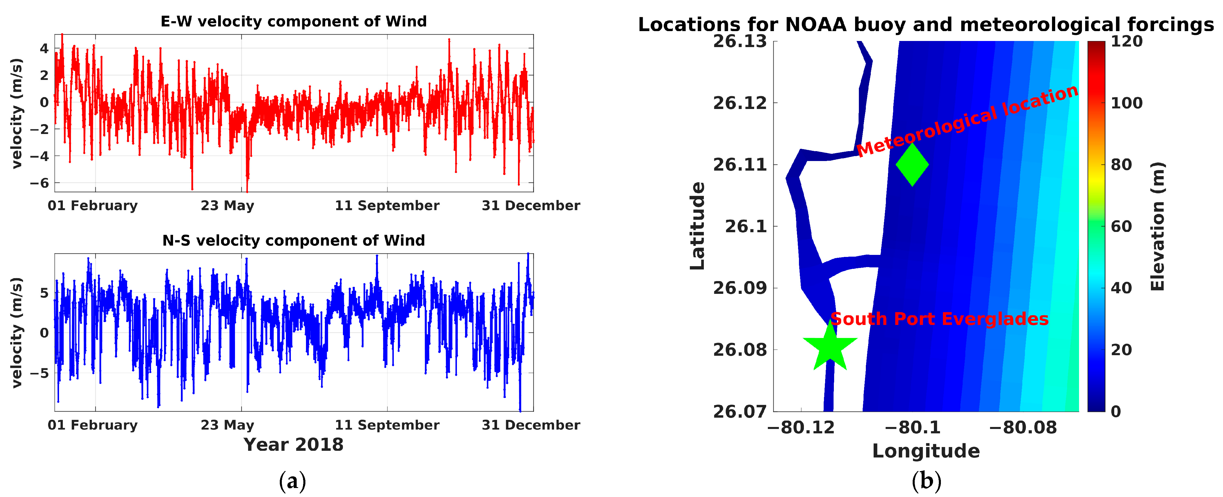
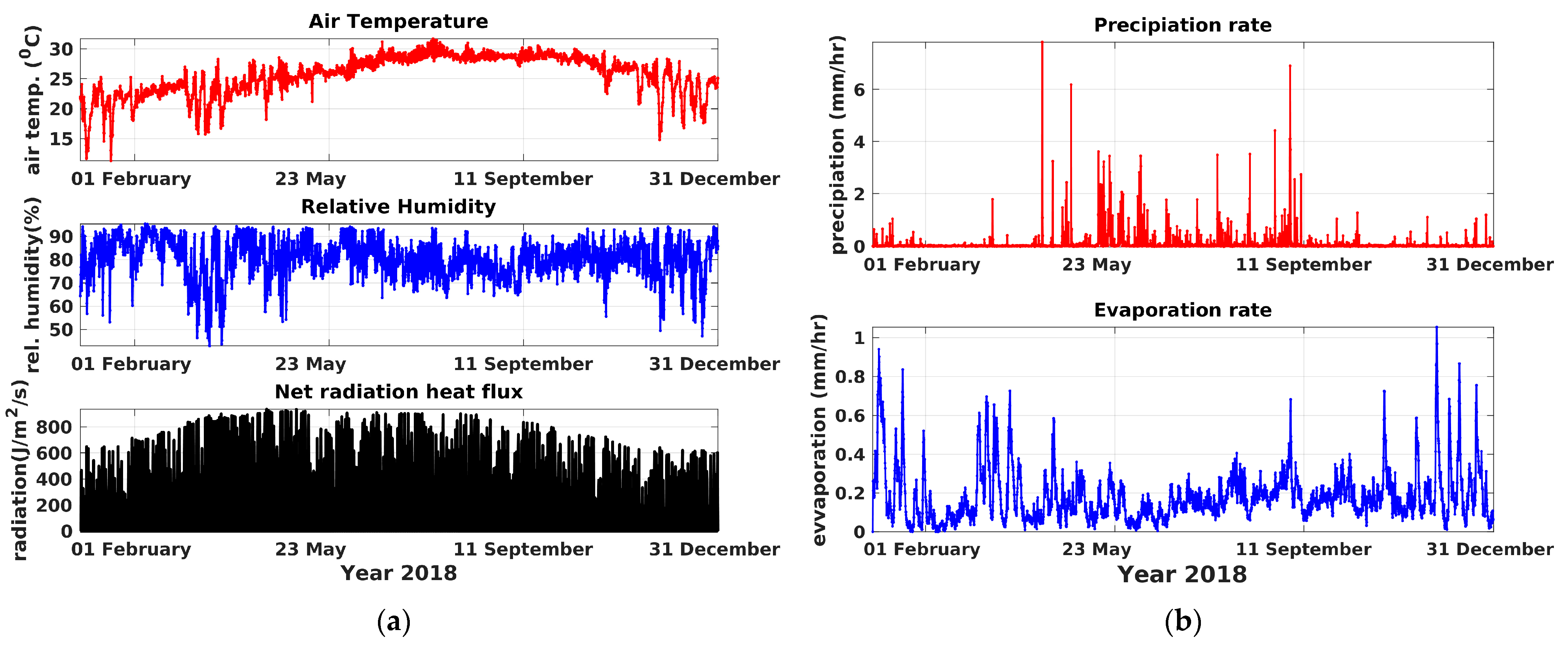
The meteorological forcings for the wind velocity (Figure 6a), relative humidity, air temperature, heat flux radiation (Figure 7a), evaporation rate, and precipitation rate (Figure 7b) were derived from the NARR model [18]. All meteorological forcing data were downloaded for a single location (green-colored diamond shape in Figure 6b). The meteorological forcings were applied uniformly over the model domain.
The absolute flux model (based on the total solar radiation) was applied for heat flux formulation. The absolute flux model [19] involves prescribing the incoming (short-wave) solar radiation while computing the net atmospheric (long wave) radiation and the heat losses resulting from evaporation, outgoing radiation, and convection (Equation (1)). The total heat flux through the free surface is defined as [9]:
Q t o t = Q s n + Q a n Q b r Q e v Q c o
where Q s n   is the net solar radiation, Q a n is the net atmospheric radiation, Q b r   is the back radiation, Q e v is the evaporative heat flux, and Q c o is the convective heat flux.

3. Model Adjustments and Calibration

A two-year (2018–2019) simulation was conducted to calibrate the model. A series of numerical experiments were performed to test the effects of the bottom friction, vertical resolution, spatial variability of surface winds, and quality of the nested model. To calibrate the model, several steps were taken: (1) the bottom friction parameter, which was critical to correctly simulating bottom friction effects in shallow water systems, was evaluated; (2) spatially variable surface wind was applied; (3) the effect of the vertical resolution of the model was also evaluated; (4) the performance of the flow model was evaluated with different boundary condition data. In the control experiment, the model was nested into the HYCOM, which had 5 vertical layers along with a Chezy parameter of 55 and was forced with 2-D winds. Three experiments were run by (1) changing the bottom friction parameters to 55, 80, and 100; (2) changing the total number of vertical layers from 5 to 10; (3) using 1-D winds, i.e., spatially uniform winds, from a chosen location (see location in Figure 6b); and (4) nesting into the regional ADCIRC model. The other parameters remained unchanged. The results from these experiments and the control experiments were compared focusing on the Port Everglades inlet. In the following sections, all figures represent a shorter time period of data (1 to 3 months) for better visualization. The model outputs from all calibration runs were compared with NOAA buoy data [20] from South Port Everglades (see location in Figure 6b).

3.1. Bottom Roughness

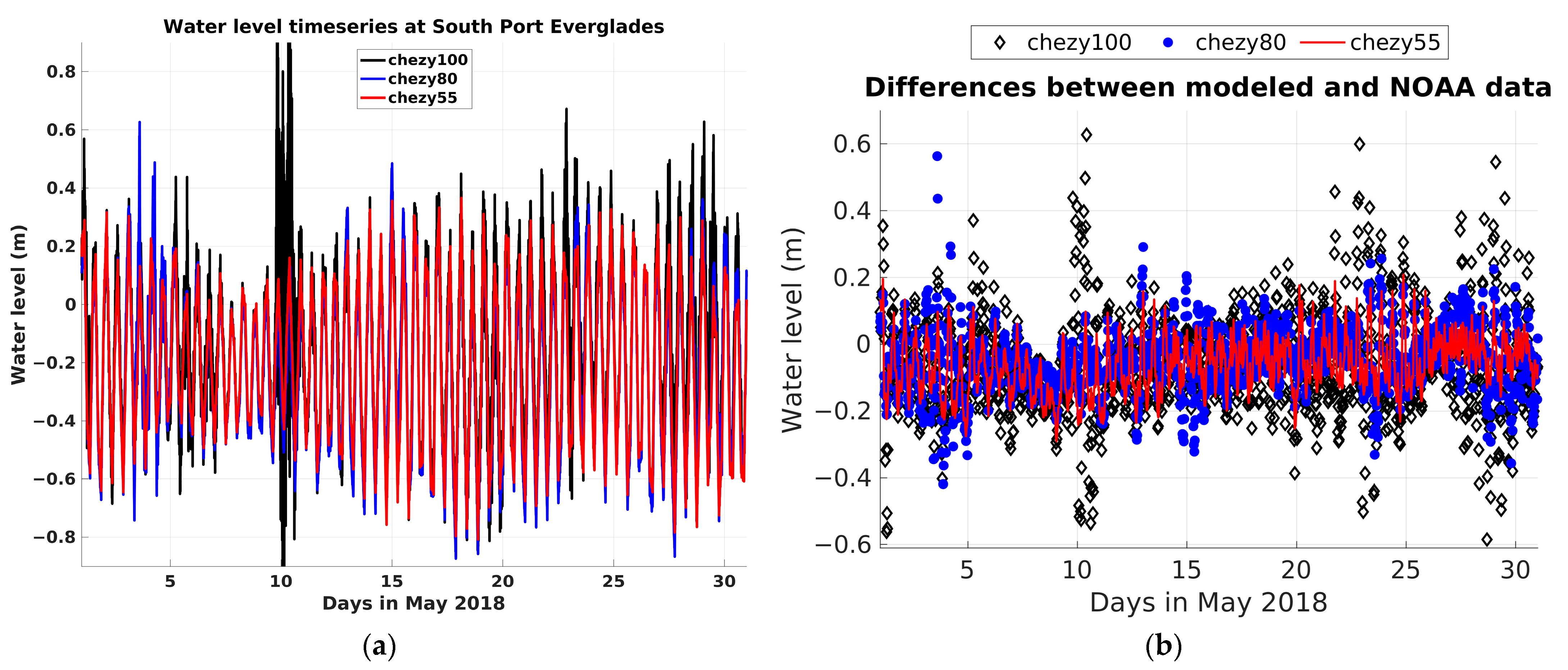
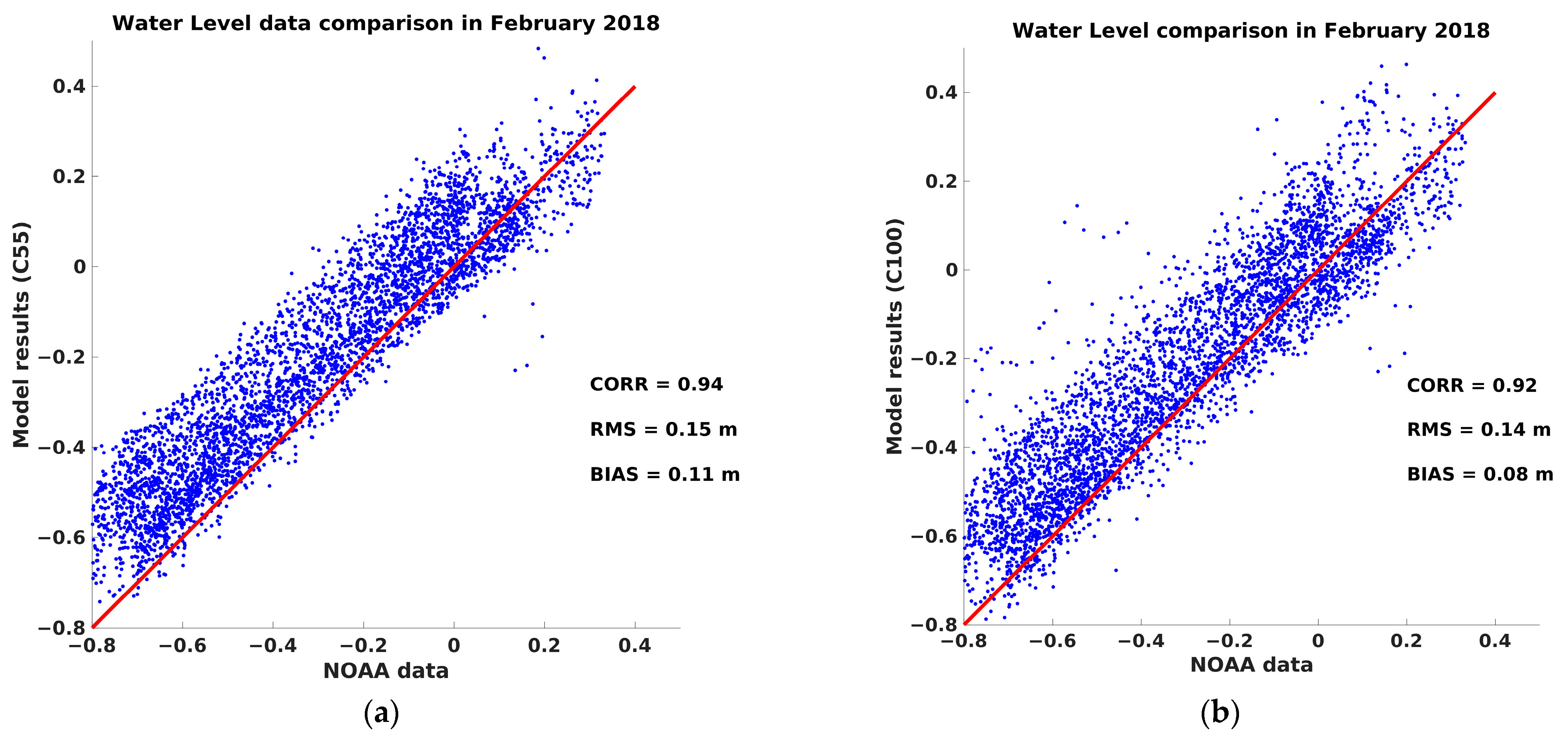
The Chezy coefficient, a parameter representing bottom roughness, was calculated using the Chezy and Manning formulations (Equations (A6) and (A7)). The Chezy roughness formulation (Equation (A6)) yielded better results. The default value for the Chezy coefficient is 65. Uniform Chezy coefficients were applied in both the north–south and west–east directions. Based on these formulas and the modeled water depth, the Chezy coefficient values ranged from 53 to 102. The effects of bottom roughness were evaluated by employing different Chezy coefficient values (55, 80, and 100) and comparing the model’s output with observed water level data obtained from the NOAA (Figure 8 and Figure 9). A time series analysis (Figure 8a,b) and statistical parameters, including correlation coefficients, the root mean square error, and the bias, were employed to assess the model’s performance (Figure 9a,b).
The comparison between the model’s output and observed data at various Chezy parameter values demonstrated that increasing the Chezy coefficient above 50 improved the correlation between the model and the observed water levels (Figure 9a,b), while reducing the differences between the modeled and the observed data (Figure 8b). However, when the parameter exceeded 80, the correlation and alignment between the model and the observed data deteriorated. Based on these findings, the optimal Chezy parameter value was determined to be 55, as it exhibited the highest model–data correlation coefficients and better alignment with the center line. The subsequent model experiments were conducted using a Chezy parameter of 55.

3.2. Five- vs. Ten-Layer Simulations

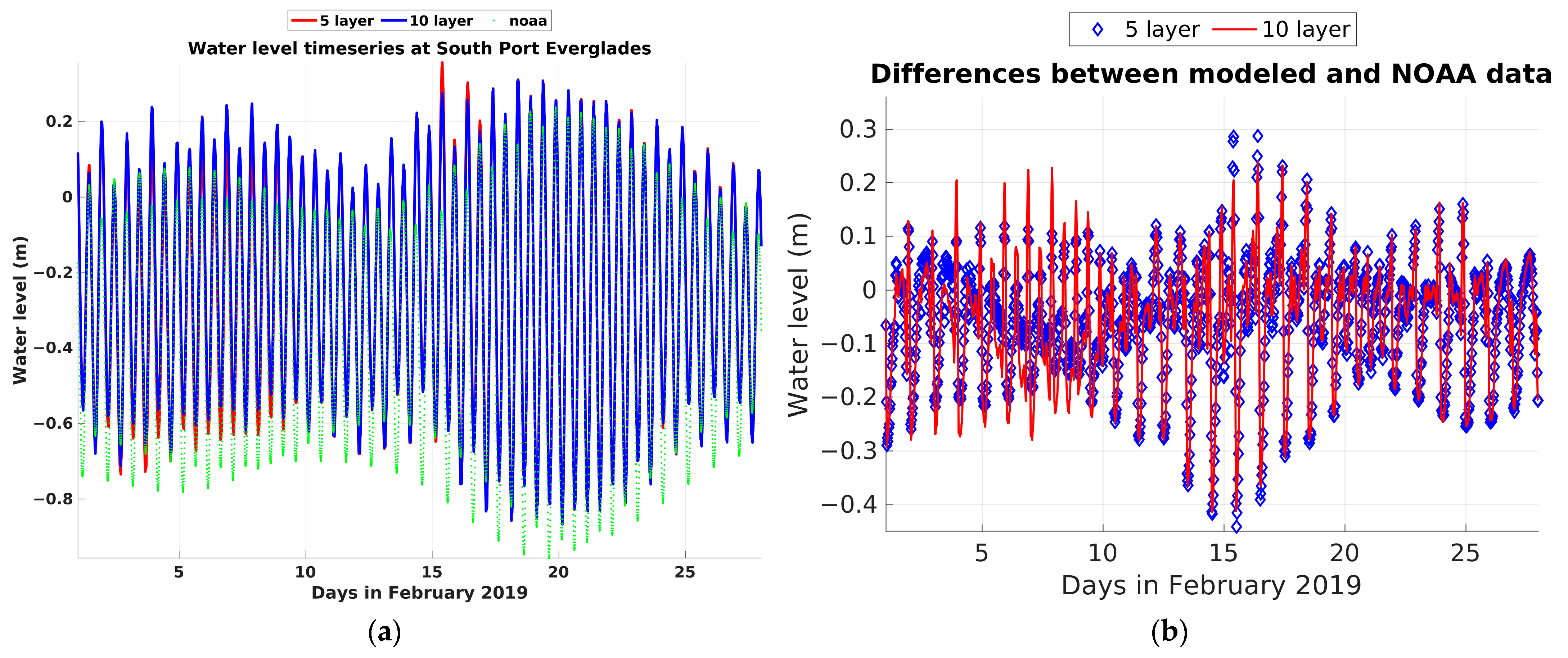
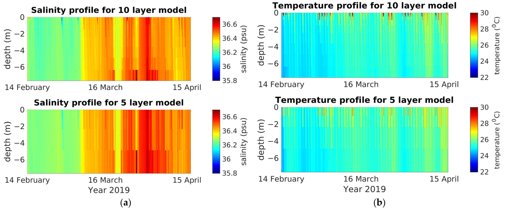
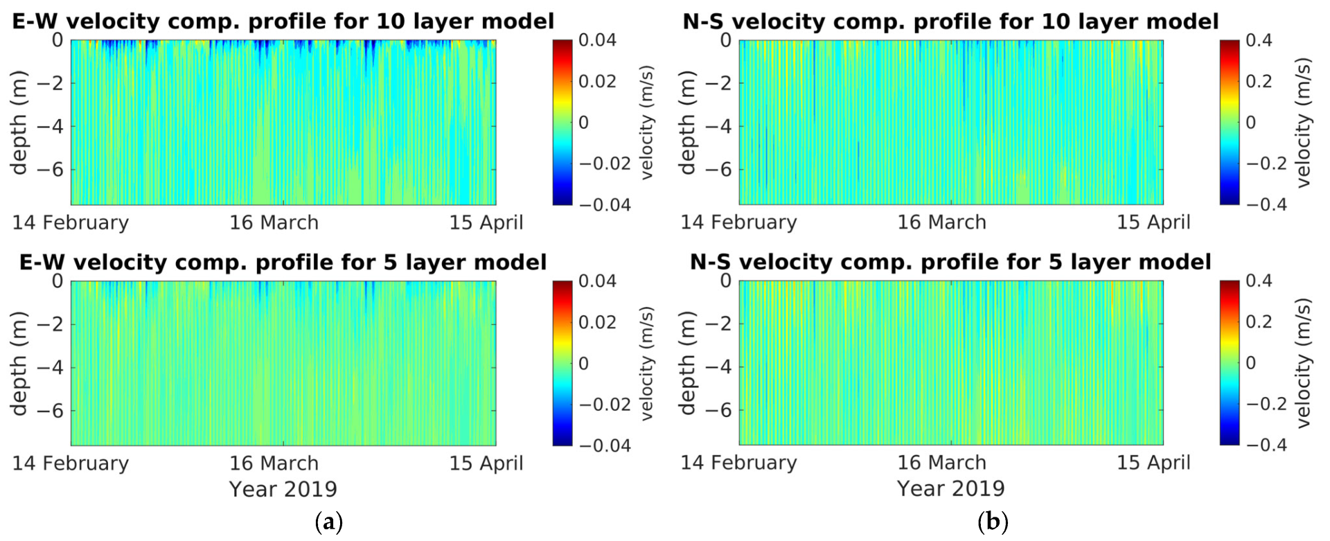
The comparison of the water level time series between the observations and the two experiments, the 10-layer model and the control (5-layer) model, reveals a minor difference in water level (Figure 10a). The discrepancies between the modeled and observed water levels are approximately 0.1 m smaller in the 10-layer model compared to the 5-layer model (Figure 10b). However, when examining the vertical profiles of salinity and temperature in the South Port Everglades, it is evident that the 10-layer model does not significantly improve the vertical stratification (Figure 11a,b). The same holds true for the horizontal velocity profile, where the 10-layer model shows only a slight improvement in vertical stratification near the surface layer (Figure 12a,b).
Although the 10-layer model performs slightly better in simulating the water level and horizontal velocity compared to the 5-layer model, the computational time required for the 5-layer model is significantly less. Considering that the change in vertical resolution did not lead to a significant improvement in model performance, the 5-layer model was selected for future simulations due to its computational efficiency.

3.3. Uniform (1-D) vs. 2-D Winds

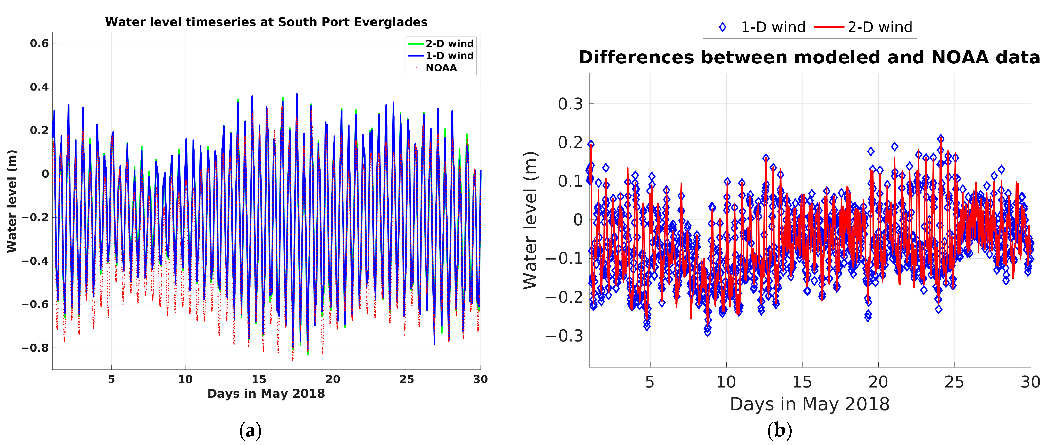
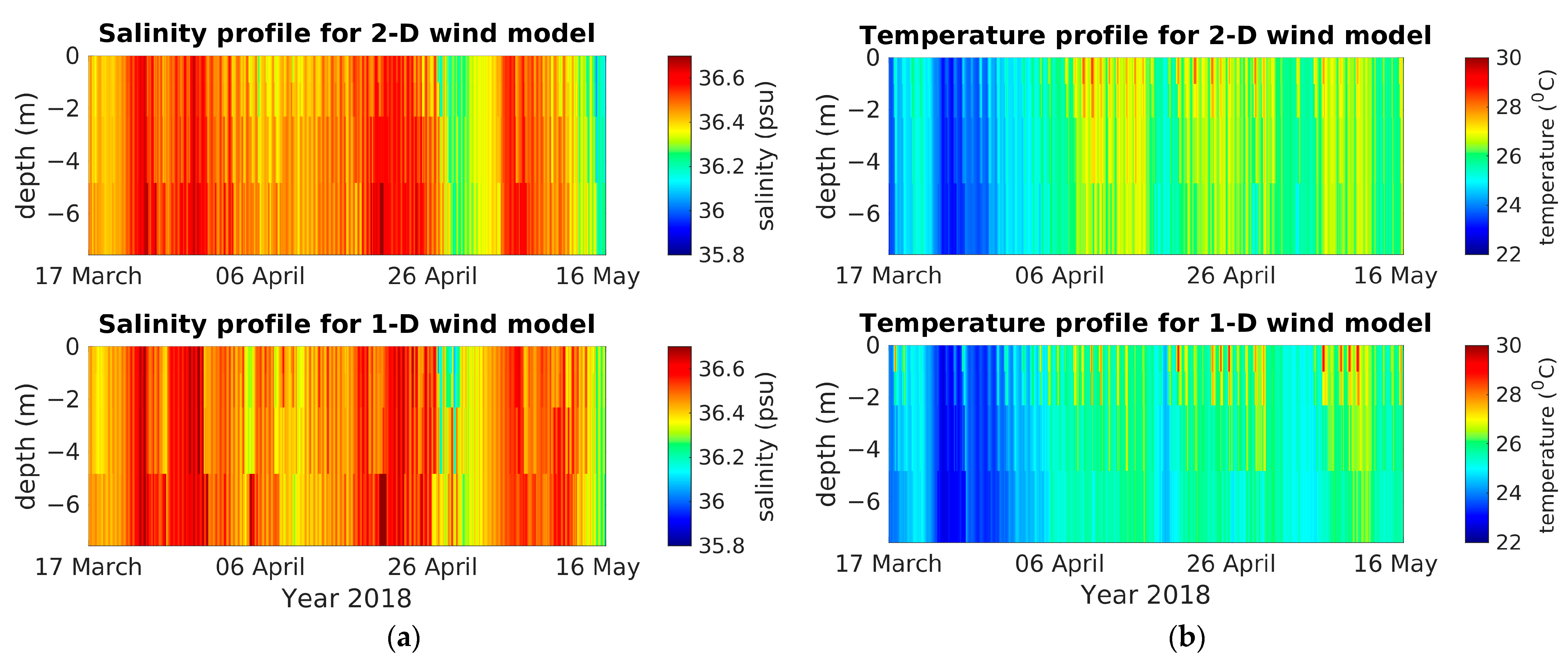
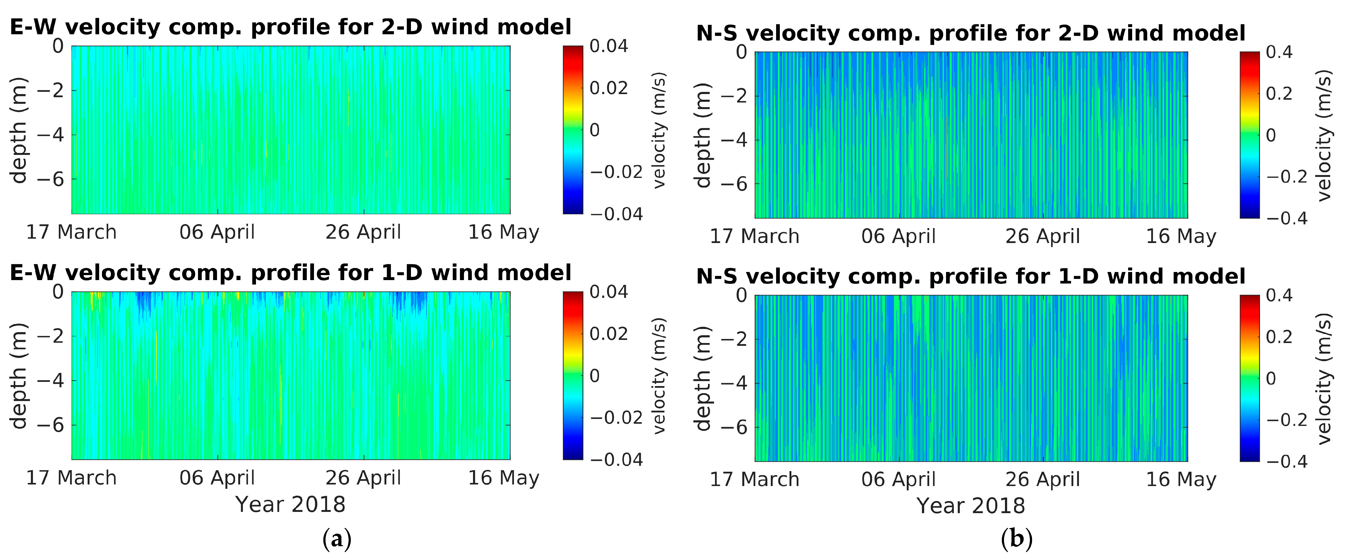
The wind experiments included two separate simulations, one with uniform wind data (1-D) and another with spatially varying wind data (2-D). The model results for the 1-D wind and 2-D wind were compared in terms of time series plots (Figure 13) of the water levels and vertical profiles (Figure 14 and Figure 15) for the salinity, temperature, and horizontal velocity in the South Port Everglades. The discrepancies between the modeled and observed water levels were approximately ~0.1 m smaller in the 2-D wind model compared to the 1-D wind model (Figure 13b). The vertical profiles (Figure 14 and Figure 15) for salinity, temperature, and horizontal velocity were examined in the South Port Everglades. In the case of salinity, the 3-D plot displayed a similar pattern along the water depth profile, except for the beginning of May, when freshwater from the surface layer dispersed throughout the profile (Figure 14a). The temperature and velocity profiles of the 2-D wind model demonstrated more prominent surface layer temperature and velocity characteristics compared to the model using 1-D wind data (Figure 14b and Figure 15a,b). This suggested that the spatially varying wind data influenced the surface layer dynamics. The use of spatially varying wind data in the 2-D wind model resulted in more pronounced surface layer characteristics in terms of the temperature and velocity profiles.

3.4. HYCOM vs. ADCIRC Model Data

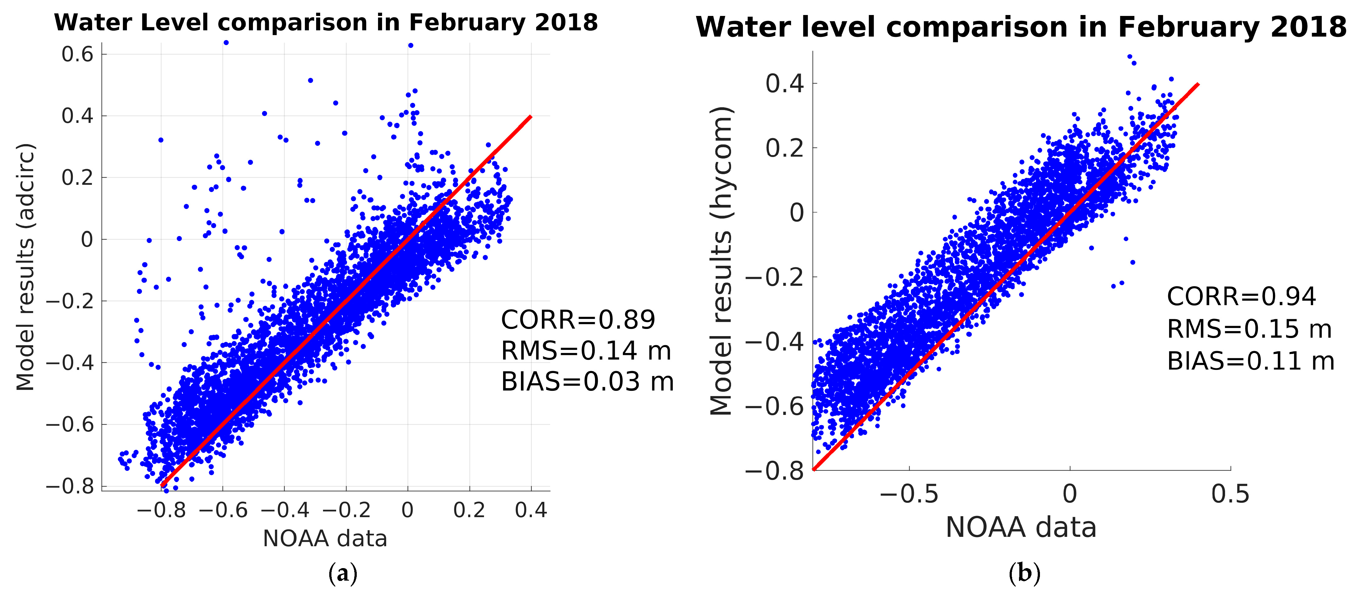
To investigate the performance of the Delft3D flow model with different boundary condition data, two simulations were conducted. In the first simulation, the water level boundary condition derived from the regional ADCIRC model [21] was utilized, while in the second simulation, water level boundary condition data from the HYCOM global model were applied. The model outputs from both simulations were then compared with NOAA water level data through a time series analysis and correlation comparison, as shown in Figure 16 and Figure 17. The time series analysis revealed that both models exhibited a correlation with the observed data. However, a notable difference in amplitudes was observed (Figure 16a). The water level differences between the model with ADCIRC data and the observations (NOAA) were often larger than those of the model with the HYCOM data (Figure 16b). The correlation comparison (Figure 17a,b) further confirmed that the model with the HYCOM boundary conditions performed better, with a higher correlation coefficient (0.94) compared to the model with the ADCIRC boundary conditions (0.89). Under similar experimental setups, the use of the HYCOM boundary conditions yielded a better match between the model outputs and observed data, with less pronounced deviations in amplitudes. Thus, the HYCOM boundary conditions demonstrated superior performance in terms of the amplitude accuracy and overall agreement with the observed data.

4. Model Performance and Skills

In this section, a series of comparisons between the model results and available measured data demonstrated the performance and skill of the model. Quantitative metrics such as the root mean square (RMS) of differences, mean difference (BIAS), and correlations (CORR) between the point-to-point model and observations were also computed to measure the differences between the model and observed data. All model results were from the control experiment.

4.1. Water Level

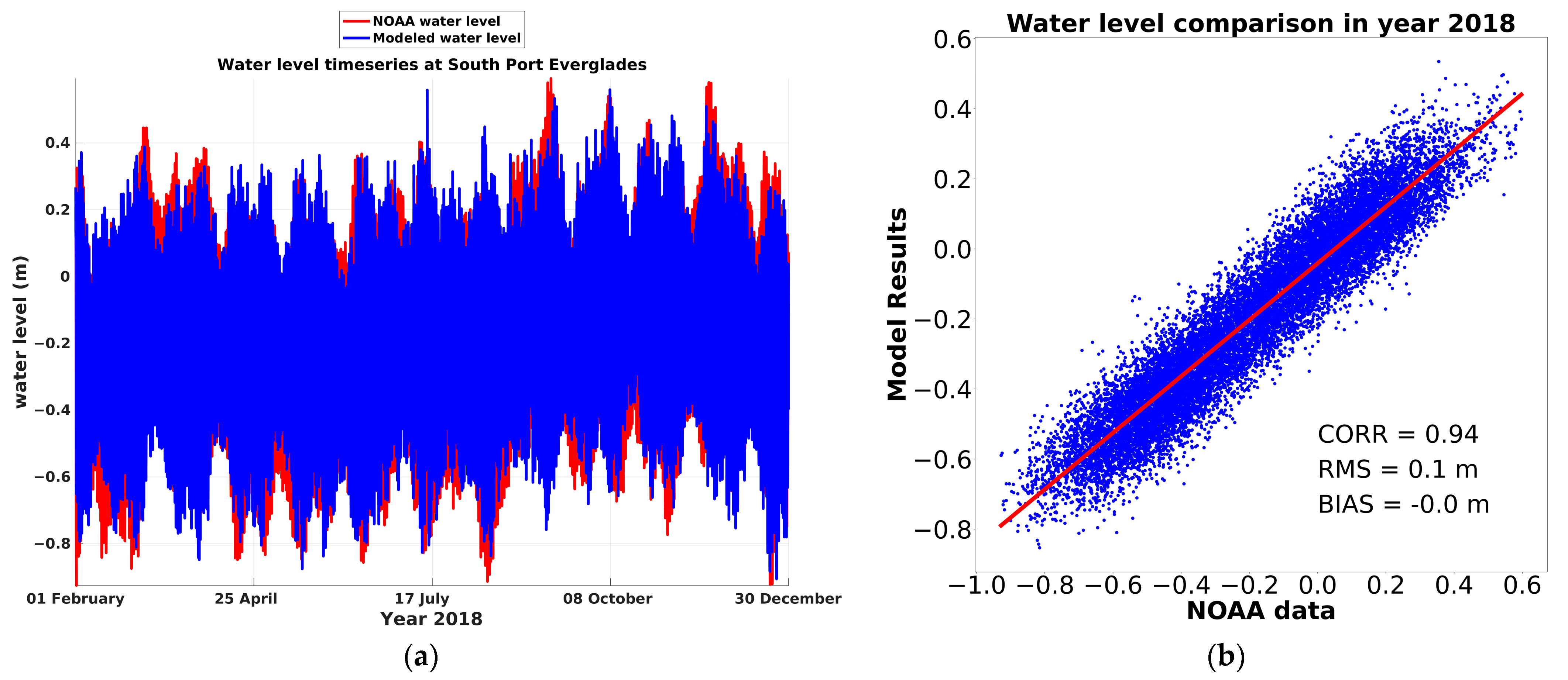
The modeled water level agreed well with the available data from the NOAA buoy at Port Everglades station (Figure 18a). The modeled and observed phases showed good agreement; however, there was a notable difference in amplitudes. The correlation comparison showed that the correlation was well over 94%, along with an RMS error of 0.1 (Figure 18b).

4.2. Salinity and Temperature

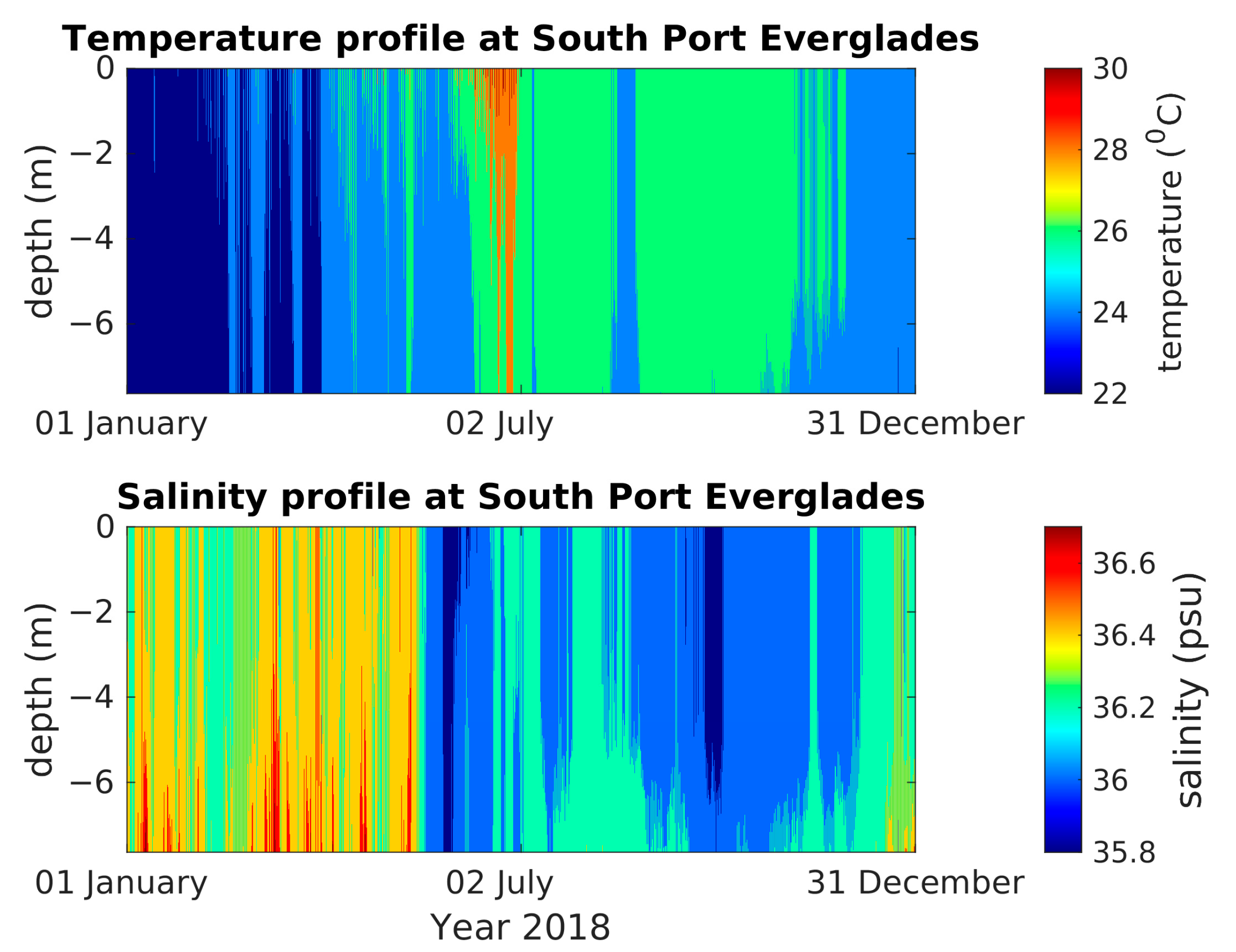
The temperature profile depicted in the top panel of Figure 19 displays expected seasonal variation. Higher water temperatures are observed during the summer months, while lower temperatures are seen during the winter months. Like the salinity patterns, the temperature variations across the depth profile are more pronounced during the summer season.
The salinity profiles in the South Port Everglades for the year 2018, as shown in the bottom panel of Figure 19, also exhibit seasonal variations. During the summer months, when there is heavy rainfall, the salinity levels are around 35 ppt. In contrast, during the winter season with less rainfall, the salinity levels increase to around 37 ppt. Notably, a salinity gradient appears during winter, while the freshwater dispersal from the surface layer disrupts this stratification during summer. The salinity and temperature profiles reveal an inverse correlation between salinity and temperature, both spatially and temporally.

4.3. Tide and Tidal Constituents

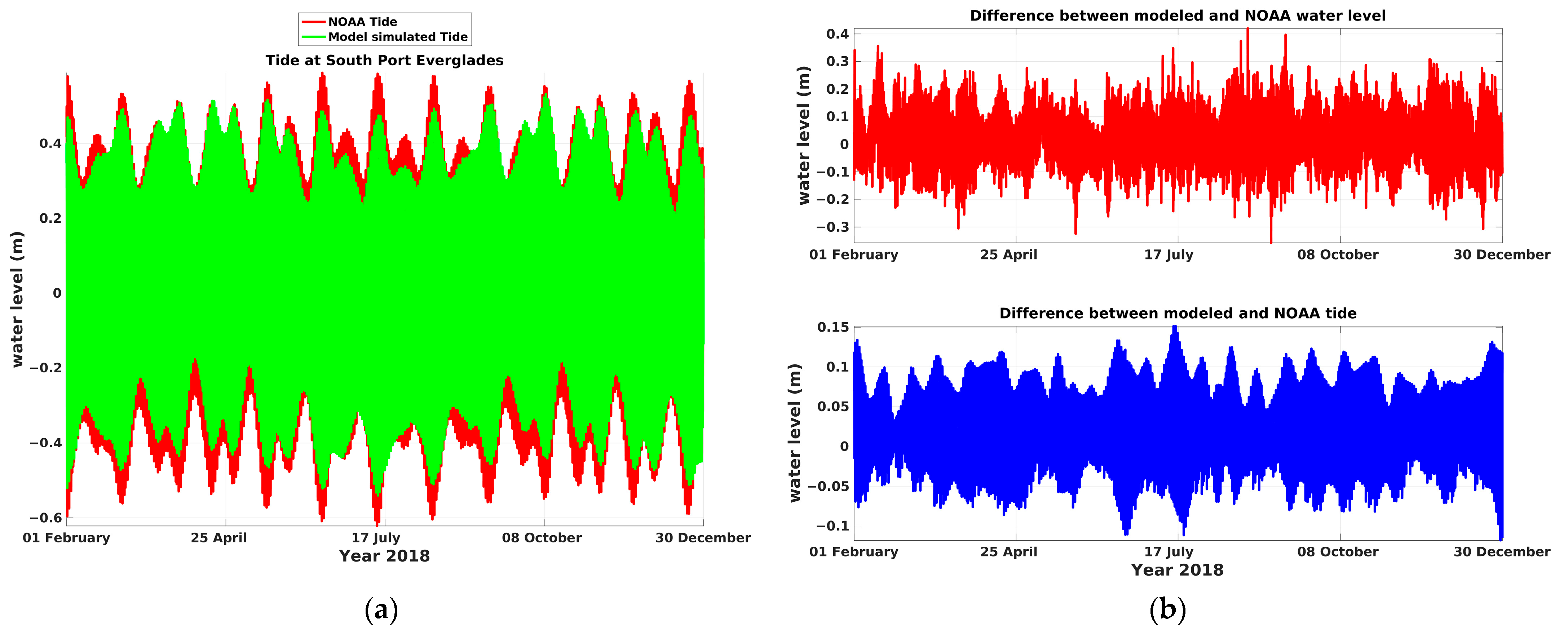
The comparison between the modeled and NOAA tide data in the South Port Everglades shows a close agreement between them (Figure 20a), with differences ranging from −0.1 to 0.1 m (bottom panel in Figure 20b). This is a better match compared to the differences between the modeled and NOAA water levels, which range from −0.3 to 0.4 m (top panel in Figure 20b). This indicates that the difference in water level data is not solely due to tidal forcings but is influenced by non-tidal forcings as well. To further investigate this, a comparison between the non-tidal components of the water level was conducted.
Figure 21 illustrates the distributions of surface salinity and currents during flood tide and ebb tide phases. It can be observed that tidal currents bring offshore high-salinity water into Port Everglades during flood tides (Figure 21b), while the saltwater plume retreats during ebb tides (Figure 21a).
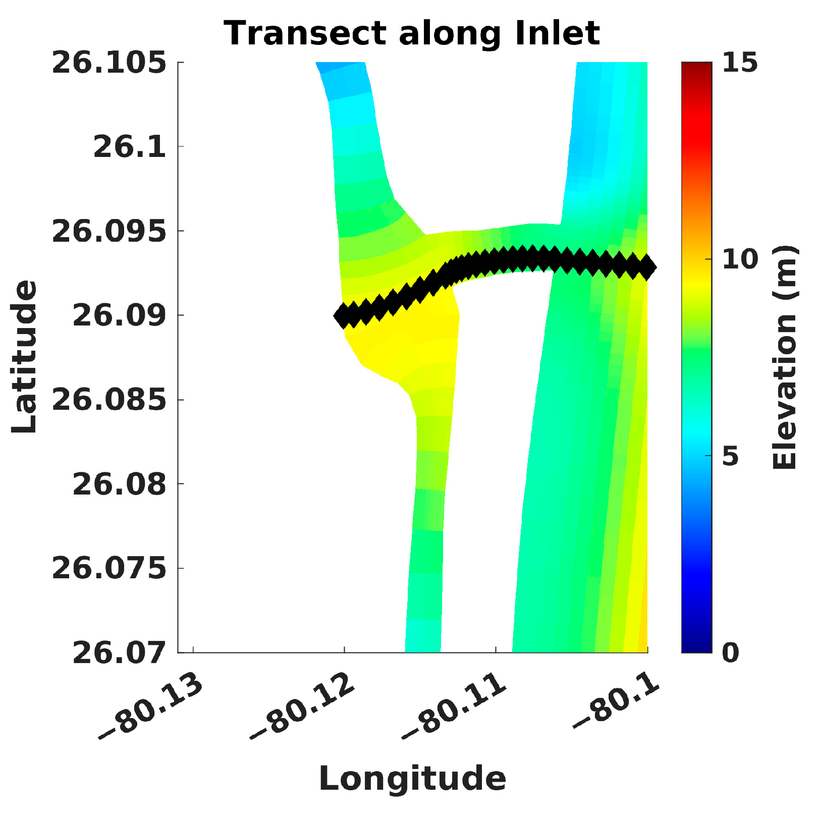
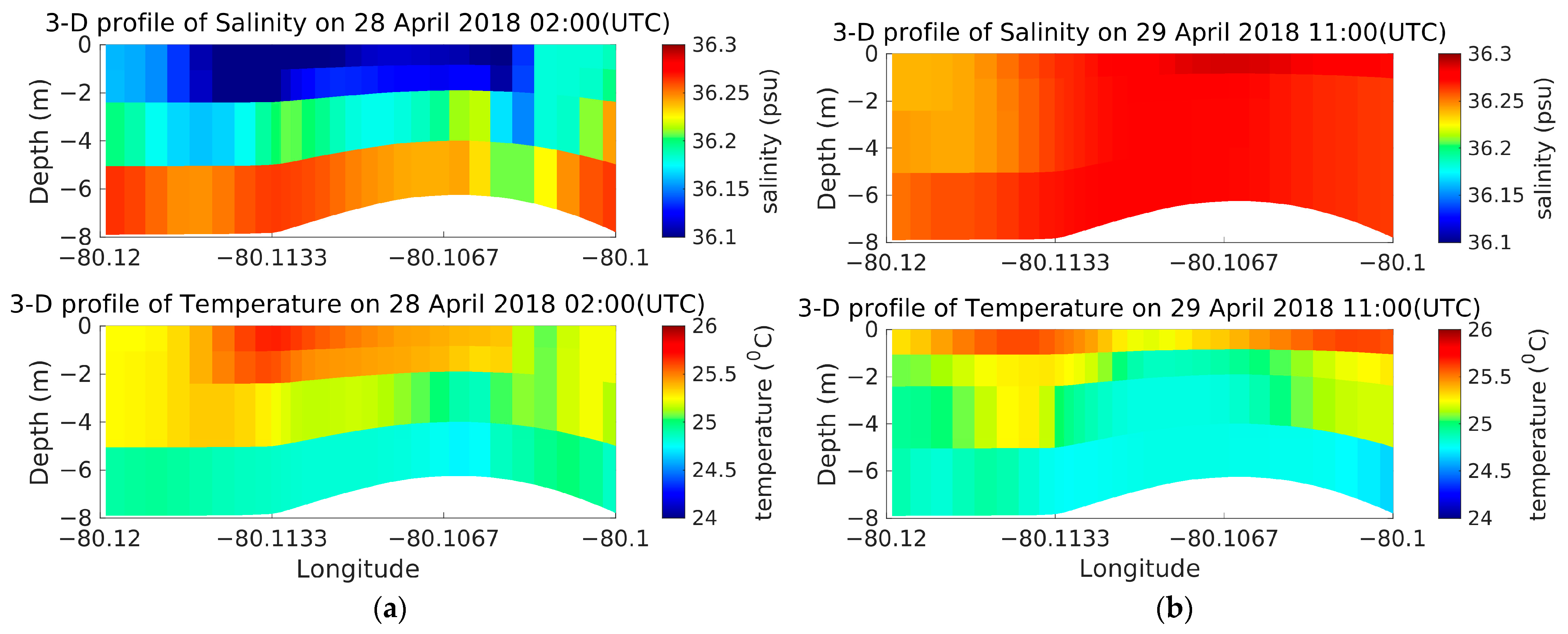
A transect (Figure 22) across Port Everglades inlet, from the inlet entrance into the coastal area to the end of the port into the harbor, was selected to visualize the distribution of hydrodynamics parameters during two distinct tide phases. Vertical profiles of salinity, temperature, and horizontal velocity are plotted along this transect line during the flood tide and ebb tide (Figure 23 and Figure 24). During the ebb tidal cycle, the salinity and temperature profiles are stratified as surface freshwater mixes into the depth profile (Figure 23a), while during the flood tidal cycle, saltwater from the ocean gets mixed throughout the profile and the stratification collapses (Figure 23b). The vertical profile of the u component of the horizontal velocity is stronger in the middle of the inlet during both tidal phases (Figure 24a,b). The velocity profile during the flood tide shows that the u component of the horizontal velocity moves toward the harbor, while during the ebb tide it moves towards the ocean. The N-S component of the horizontal velocity is weaker compared to the E-W velocity component during both tidal phases due to the geometrical constraints of the inlet (Figure 24a,b).
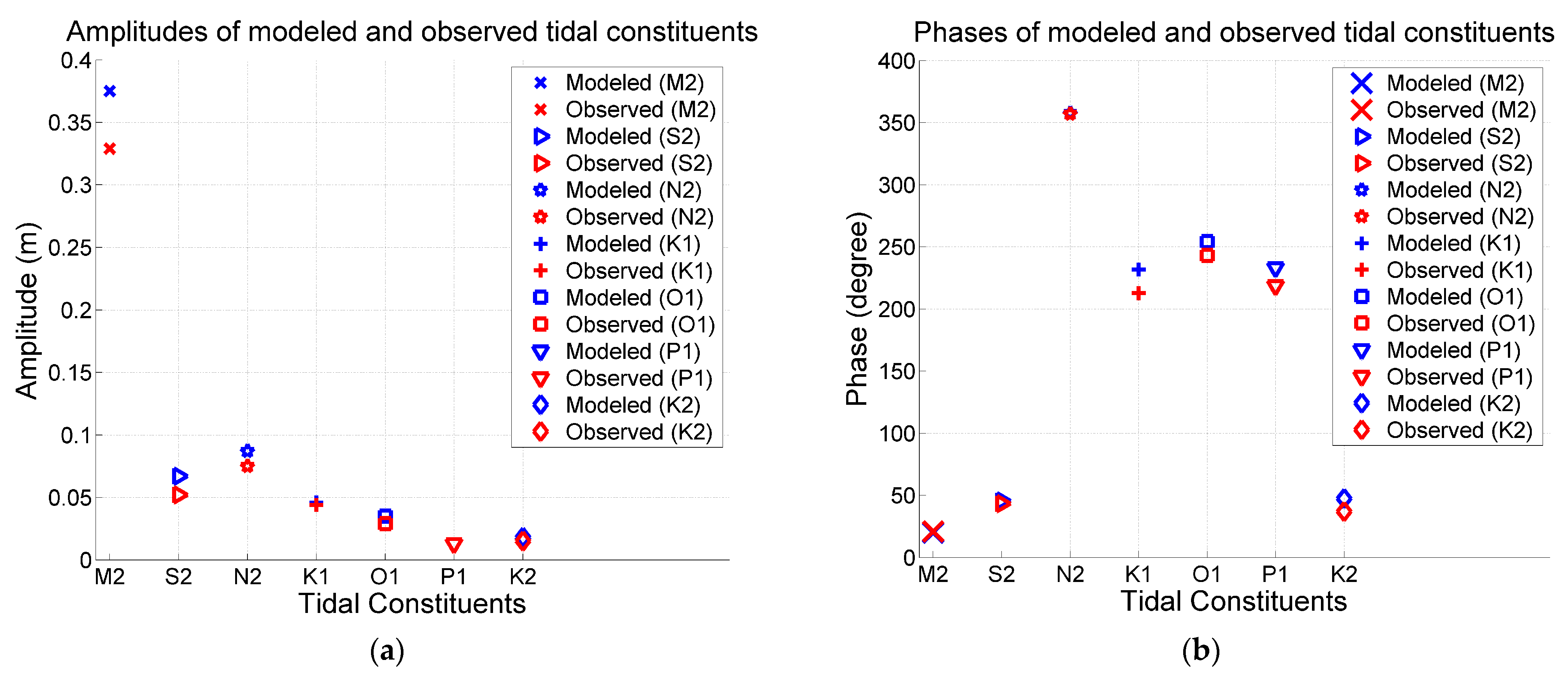
The dominant tidal constituents in this study area were semi-diurnal M2, S2, and N2 and diurnal K1 and O1 constituents. The amplitudes and phases of these tidal constituents were derived from the model output using the t_tide MATLAB toolbox from [22]. The comparison between the model-simulated tidal constituents and the observed tidal constituents showed close agreement in terms of the amplitudes and phases. The tidal constituents derived from the model simulation closely aligned with the tidal constituents obtained from the NOAA data (Figure 25).

4.4. Non Tidal Flow

To compare the modeled and observed sub-tidal flow, both the modeled and observed water levels were filtered using a Lanczos low-pass filter with a cutoff period of 12.4 h, as the dominant tidal component in this area is the semi-diurnal M2 tide. An example of a comparison among the modeled and observed residuals at Port Everglades station and the residuals from the nearest HYCOM node is shown in Figure 26a. Both the modeled and HYCOM data residuals capture the overall phase of the residuals from the observed data but show a discrepancy in amplitude. It is also evident that the modeled residuals are closely related to the HYCOM residuals. This was further investigated by comparing the differences between the modeled and observed data and the differences between the modeled and HYCOM residuals (Figure 26b). The comparison shows that the differences between the modeled and observed data are quite large compared to the differences between the modeled and HYCOM residuals. This indicates that the modeled results are as good as the HYCOM inputs. The HYCOM data do not incorporate the low-frequency sea level oscillation well. The discrepancy between the modeled and observed data can be attributed to the incomplete representation of the Gulf Stream effects in the HYCOM water level data applied to the boundary nodes. This impact on the overall water level predictions can be seen in Figure 18 and Figure 20, accounting for the offset between the model and measured water levels.

5. Real-Time Forecast

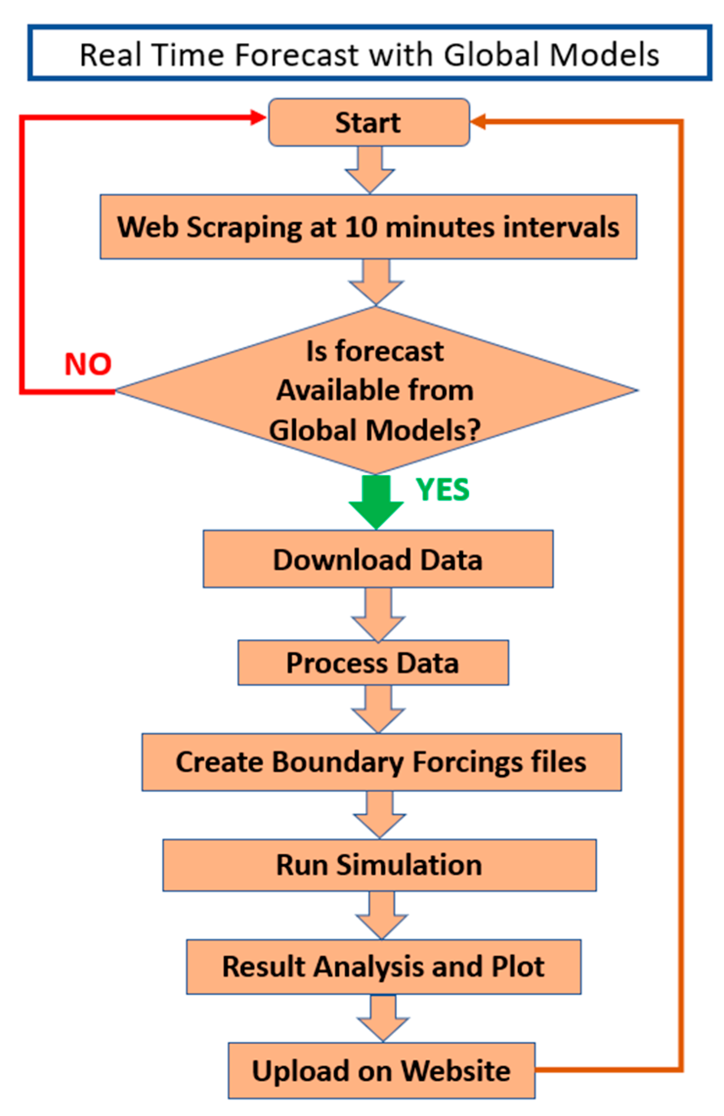
For the real-time forecast, the model boundary conditions must be updated with forecast data from the HYCOM [17] and NAM [23]. Python scripts are used for a web scraping process to extract data from websites with automation to check whether forecast data are available from global models. Whenever new forecast data are available, the new data set is downloaded for the model domain. The downloaded data are then converted and processed to create boundary conditions. A new simulation of the calibrated model is run with the forecast boundary condition files. When the simulation run is complete, the output is processed to create a time-series plot at observation stations and in coastal areas. Each time the new simulation is run with a hot start file from the previous simulation. The results from this new simulation run are uploaded to the GitHub website. These scripts are automated and synchronized in such a way that it keeps checking for new data at 10-minute intervals. If new data for the boundary conditions are available, the data will be downloaded and processed and outputs from the simulation will be processed and uploaded to the webpage. If new data are not available, it will sit idly for 10 min and be checked again, creating an endless loop (Figure 27).
The entire process is executed with bash, MATLAB, and Python scripts (Figure 28). A bash script named ‘mainf.sh’ runs all required scripts one by one, synchronizing the downloading of new data, boundary condition creation, simulation runs, and the post-processing of model simulations. First ‘check_newdata.sh’ checks whether there are new data available on the NAM website [23] using a web scraping method (using the Python library ‘beautifulsoup4’). If new data are available, a Python script ‘nam_scrap.py’ downloads the new meteorological data, ‘ncl_conversion.sh’ converts the downloaded ‘Grib2’ formatted file to the NetCDF (network common data form) format, and the MATLAB script ‘nam_process.m’ processes the NetCDF files to create meteorological boundary conditions. Next, the ‘chcek_hycom.py’ script checks whether new data are available on the HYCOM data server. If new HYCOM data are available, ‘hycom_scraping.py’ downloads salinity, temperature, and water level data in the NetCDF format for the study area. The downloaded NetCDF data are then processed to create a flow boundary conditions file using the bash script ‘hycom_process.sh’ and MATLAB script ‘create_bcc.m’. The bash script ‘run_d3d.sh’ runs a new simulation, while ‘post_process.sh’ post-processes the model results and creates visuals for all stations. Then, the ‘git_upload.sh’ scripts copy all required files into a GitHub folder and upload them to the GitHub webpage (see Supplementary Materials).

6. Discussion and Conclusions

A three-dimensional numerical model was developed using Delft3D for Port Everglades, Florida, to simulate hydrodynamics and transport. The model included high spatial resolution in the Port Everglades area. The model was driven by a water elevation time series that included tides and low-frequency sea level oscillations, meteorological forcing, and open transport boundary conditions. To calibrate the model skill, the model outputs including water level and tidal constituents were compared with the NOAA buoy data near South Port Everglades. Extensive calibration was performed for key model parameters and configurations, including the bottom roughness, bathymetry, vertical resolution, spatially varying wind, and heat flux formulation. The water level output showed slight differences (~0.1 m) between the 5-layer model and 10-layer model. The 10-layer model produced stronger E-W velocity components near the surface layer and more pronounced stratification in velocity profiles compared to the 5-layer model (Figure 12). There were marginal differences of around 0.1 m between the modeled and observed water level data with the 2-D wind forcing compared to the 1-D wind forcing. One probable reason for these insignificant differences may have been due to the low resolution of the NARR [18] model products, which were unable to represent the small-scale variability of surface winds between the river and coastal oceans. The bottom roughness parameter had significant effects on the model results. The calibration of the model with different values showed that the best results were achieved when a medium-range roughness (55) was used (Figure 8 and Figure 9).
After the calibration, a 2-year (2018–2019) simulation was performed. Overall, the modeled results were in good agreement with the data in terms of the major features. As an example, Figure 18 shows a comparison of the model water levels with the observed data and the South Port Everglades NOAA station data, which indicates a good agreement between the modeled results and observation. The model tidal constituents (amplitudes and phases) were also in good agreement with the NOAA tidal constituents (Figure 25). Modeled sub-tidal sea level oscillations were in general agreement with the measured sub-tidal sea level variations but did not capture shorter term variations. This was due to an incomplete representation of Gulf Stream effects in the HYCOM water level that was used for coastal boundary conditions (Figure 18 and Figure 26). Overall, the coastal model results supported by the boundary conditions from a larger basin scale model show that tidal movements, sea level variations, and surface winds are the predominant factors in controlling the circulation in the Port Everglades area and the adjacent coastal ocean.
A real-time forecast model for the Port Everglades area was developed using the calibrated Delft3D model, which predicts water level, salinity, current, and temperature results for up to 3 days. In this forecast system, the model setup, updating boundary conditions, simulations, plotting, and updating of the website occurs automatically without manual intervention. For this automation process, scripts were synchronized in such a way that they continually acquire and process data into the forecast model automatically. These scripts detect newly available data from basin-scale models, download new data, create new boundary conditions, set up a model, run forecast simulations, plot the model results, and finally upload the forecast data on the GitHub webpage (Figure 27 and Figure 28). This forecast system has been successfully running since 2019.
This forecast model is especially useful for the prediction of hydrodynamic scenarios in study areas that may impact dredging projects and other engineering activities, as well as providing the basis for an ongoing environmental analysis if coupled with model-driven water quality calculations. This study illustrates detailed methods of developing a real-time forecast model (nested in basin-scale models) for estuary and coastal regions and could serve as a guideline for the future use and development of a real-time coastal process forecast model.

Supplementary Materials

The real-time forecast for Port Everglades can be accessed through the following link: https://realtimefl.github.io/Real-Time-Forecast-Port-Everglades/ (accessed on 24 April 2023).

Author Contributions

Conceptualization, G.A.Z. and M.A.H.; methodology, M.A.H.; software, M.A.H.; validation, G.A.Z.; formal analysis, M.A.H.; investigation, M.A.H.; resources, G.A.Z.; data curation, M.A.H.; writing—original draft preparation, M.A.H.; writing—review and editing, G.A.Z. and M.A.H.; visualization, M.A.H.; supervision, G.A.Z.; project administration, G.A.Z. All authors have read and agreed to the published version of the manuscript.

Funding

This research was funded by the Florida Institute of Technology and the Sebastian Inlet Tax District.

Institutional Review Board Statement

Not applicable.

Informed Consent Statement

Not applicable.

Data Availability Statement

All automation scripts including MATLAB, bash, and Python scripts; research data; and figures are publicly available on: https://drive.google.com/drive/u/0/folders/1ANA9rtdJMloM6N0dYmLMCkZfYXILOuRV (accessed on 24 April 2023).

Acknowledgments

The authors would like to thank the Sebastian Inlet Tax District for supporting this research and the reviewers for their insightful comments.

Conflicts of Interest

The authors declare no conflict of interest.

Appendix A

Open boundary conditions
The available types of open boundary conditions for coastal and estuarine models include water level, velocity, water level gradient, discharge, and Riemann conditions. To make these boundary conditions weakly reflective, a reflection coefficient, denoted as alpha ( α ), is specified. This coefficient alpha must be greater than or equal to 0 [15,16]. The reflection coefficient ensures that outgoing waves from the model do not reflect at the boundary and cause disturbances within the model domain. It is important to note that the reflection parameter does not apply to Riemann boundary conditions. Stelling [24] introduced the time derivative of the Riemann invariant to the water level (Equation (A1)) and velocity boundary conditions. This modification helps to reduce the reflective nature of the boundaries for disturbances with the Eigen frequency of the model area. This reduces the spin-up time of a model from a cold start [9]. The time derivative to the water level boundary is defined as follows [9]:
ζ + α t U ± 2 g H = F ζ t
where H is the water depth, g is the gravity, and α is the reflection coefficient, which is described as follows [9]:
α = T d H g
where the parameter T d represents the travel time of a free surface wave across the model domain from the left boundary to the right boundary. In ocean and sea models, the period T d   is typically of the same order as the period of the tidal forcing. In these cases, it is crucial to set the reflection coefficient α to 0. This is necessary because a non-zero α would reduce the amplitude of one of the components in the boundary condition [9].
Bottom roughness
The bottom friction is specified in the boundary conditions (Equations (A3) and (A4)) for the momentum equations. The bottom friction is approximated by a quadratic friction law (Equation (A5)). The boundary conditions for the momentum equations at the bottom are defined as follows [9]:
ν V d   + ζ u σ σ = 1 = 1 ρ 0 τ b ξ
ν V d   + ζ v σ σ = 1 = 1 ρ 0 τ b η
where τ b ξ is the component of the bed stress in the ξ direction and τ b η is the component of the bed stress in the η direction, σ = 1 indicates bottom surface in the σ coordinate system, ρ 0 is the density of water, ζ is the water level, d is the depth, v V is the vertical eddy viscosity, and u and v represent the flow velocities in the ξ and η direction, respectively.
The shear stress for the 2-D depth-averaged flow at the bottom, induced by a turbulent flow, is assumed by a quadratic friction law [9]:
τ b = ρ 0 g U U C 2 D 2
where τ b is the shear stress at the bed, U is the magnitude of the depth-averaged horizontal velocity, g is the gravity, and C 2 D is the 2-D Chezy coefficient.
After performing depth average calculations, the 3-D calculations are carried out in the model. In this context, the 2-D Chezy coefficient ( C 2 D ) can be employed to calibrate the water level in a 3-D model, assuming a logarithmic distribution for the vertical profile of the horizontal velocity (e.g., tidal flows in estuaries and seas) [9].
The Chezy coefficient C 2 D for the depth-averaged flow is defined as follows [9]:
C 2 D = g κ ln 1 + H e z 0  
where z 0 is the roughness height, κ is the Von Karman constant, and H is the total water depth, H = d   + ζ .
The Manning formulation for the Chezy coefficient ( C 2 D ) is calculated as follows [9]:
C 2 D = H 6 n
where n is the Manning coefficient.

References

  1. Auclair, F.; Estournel, C.; Marsaleix, P.; Pairaud, I. On coastal ocean embedded modeling. Geophys. Res. Lett. 2006, 33, 14. [Google Scholar] [CrossRef]
  2. Beckers, J.M.; Brasseur, P.; Nihoul, J. Circulation of the western mediterranean: From global to regional scales. Deep Sea Res. Part II Top. Stud. Oceanogr. 1997, 44, 531–549. [Google Scholar] [CrossRef]
  3. Cailleau, S.; Fedorenko, V.; Barnier, B.; Blayo, E.; Debreu, L. Comparison of different numerical methods used to handle the open boundary of a regional ocean circulation model of the Bay of Biscay. Ocean Model. 2008, 25, 1–16. [Google Scholar] [CrossRef]
  4. Penven, P.; Debreu, L.; Marchesiello, P.; McWilliams, J.C. Evaluation and application of the ROMS 1-way embedding procedure to the central California upwelling system. Ocean Model. 2006, 12, 157–187. [Google Scholar] [CrossRef]
  5. Katavouta, A.; Thompson, K. Downscaling Ocean conditions: Experiments with a quasi-geostrophic model. Ocean Model. 2013, 72, 231–241. [Google Scholar] [CrossRef]
  6. Katavouta, A.; Thompson, K.R.; Lu, Y.; Loder, J.W. Interaction between the tidal and seasonal variability of the Gulf of Maine and Scotian shelf region. J. Phys. Oceanogr. 2016, 46, 3279–3298. [Google Scholar] [CrossRef] [Green Version]
  7. Ezer, T.; Atkinson, L.P.; Corlett, W.B.; Blanco, J.L. Gulf stream’s induced sea level rise and variability along the us mid-Atlantic coast. J. Geophys. Res. Ocean 2013, 118, 685–697. [Google Scholar] [CrossRef] [Green Version]
  8. Tomczak, M. Shelf and Coastal Oceanography; University of Maine: Orono, ME, USA, 1998. [Google Scholar]
  9. Deltares, D. Simulation of Multi-Dimensional Hydrodynamic Flows and Transport Phenomena, Including Sediments; Version 4.05; Delft3D-Flow User Manual: Delft, The Netherlands, 2022. Available online: https://oss.deltares.nl/web/delft3d/manuals (accessed on 16 February 2023).
  10. Google Earth, Version 9.185.0.0. Port Everglades, Florida, USA. Available online: https://earth.google.com (accessed on 20 March 2023).
  11. NOAA National Geophysical Data Center. 1/3 Arc-Second MHW Coastal Digital Elevation Model; NOAA National Centers for Environmental Information: Palm Beach, FL, USA, 2010. Available online: https://www.ncei.noaa.gov/access/metadata/landing-page/bin/iso?id=gov.noaa.ngdc.mgg.dem:427 (accessed on 25 April 2018).
  12. Leendertse, J.J. Aspects of a Computational Model for Long-Period Water-Wave Propagation; RAND Corp.: Santa Monica, CA, USA, 1967. [Google Scholar]
  13. Leendertse, J.J.; Gritton, E.C. A Water-Quality Simulation Model for Well Mixed Estuaries and Coastal Seas: Volume II: Computation Procedures; RAND Corp.: Santa Monica, CA, USA, 1971; p. 53. [Google Scholar]
  14. Leendertse, J.J.; Alexander, R.C.; Liu, S.K. A Three-Dimensional Model for Estuaries and Coastal Seas: Volume I, Principles of Computation; RAND Corp.: Santa Monica, CA, USA, 1973. [Google Scholar]
  15. Verboom, G.K.; Slob, A. Weakly reflective boundary conditions for two-dimensional shallow water flow problems. Adv. Water Resour. 1984, 7, 192–197. [Google Scholar] [CrossRef]
  16. Verboom, G.K.; Segal, A. Weakly-reflective boundary conditions for shallow water equations. In Research in Numerical Fluid Mechanics; Vieweg+Teubner Verlag: Wiesbaden, Germany, 1987. [Google Scholar]
  17. Metzger, E.J.; Helber, R.W.; Hogan, P.J.; Posey, P.G.; Thoppil, P.G.; Townsend, T.L.; Wallcraft, A.J.; Smedstad, O.M.; Franklin, D.S.; Zamudo-Lopez, L.; et al. Global Ocean Forecast System 3.1 Validation Testing; NRL Report; Naval Research Lab Stennis Detachment: Stennis Space Center, MS, USA, 2017; NRL/MR/7320--17-9722. Available online: https://hycom.org (accessed on 24 March 2023).
  18. Mesinger, F.; DiMego, G.; Kalnay, E.; Mitchell, K.; Shafran, P.C.; Ebisuzaki, W.; Jović, D.; Woollen, J.; Rogers, E.; Berbery, E.H.; et al. North American Regional Reanalysis: A long-term, consistent, high-resolution climate dataset for the North American domain, as a major improvement upon the earlier global reanalysis datasets in both resolution and accuracy. Bull. Am. Meteorol. Soc. 2006, 87, 343–360. [Google Scholar] [CrossRef] [Green Version]
  19. Octavio, K.A.H.; Jirka, G.H.; Harleman, D.R.F. Vertical Heat Transport Mechanisms in Lakes and Reservoirs. Ph.D. Thesis, Massachusetts Institute of Technology, Cambridge, MA, USA, 1977. [Google Scholar]
  20. NOAA Tides and Currents. South Port Everglades, FL—Station ID: 8722956. Available online: https://tidesandcurrents.noaa.gov/waterlevels.html?id=8722956 (accessed on 5 June 2018).
  21. Real Time Florida Coastal Guidance. East Central Coast, Indian River Lagoon, and Brevard County. Available online: https://fl-asgs.github.io/ECFL-IRL/ (accessed on 27 July 2018).
  22. Pawlowicz, R.; Beardsley, B.; Lentz, S. Classical tidal harmonic analysis including error estimates in MATLAB using T_TIDE. Comput. Geosci. 2002, 28, 929–937. [Google Scholar] [CrossRef]
  23. NOAA. North American Mesoscale Forecast System (NAM). Available online: https://registry.opendata.aws/noaa-nam (accessed on 24 March 2023).
  24. Stelling, G.S. On the Construction of Computational Methods for Shallow Water Flow Problems. Ph.D. Thesis, Rijkswaterstaat, Utrecht, The Netherlands, 1983. [Google Scholar]
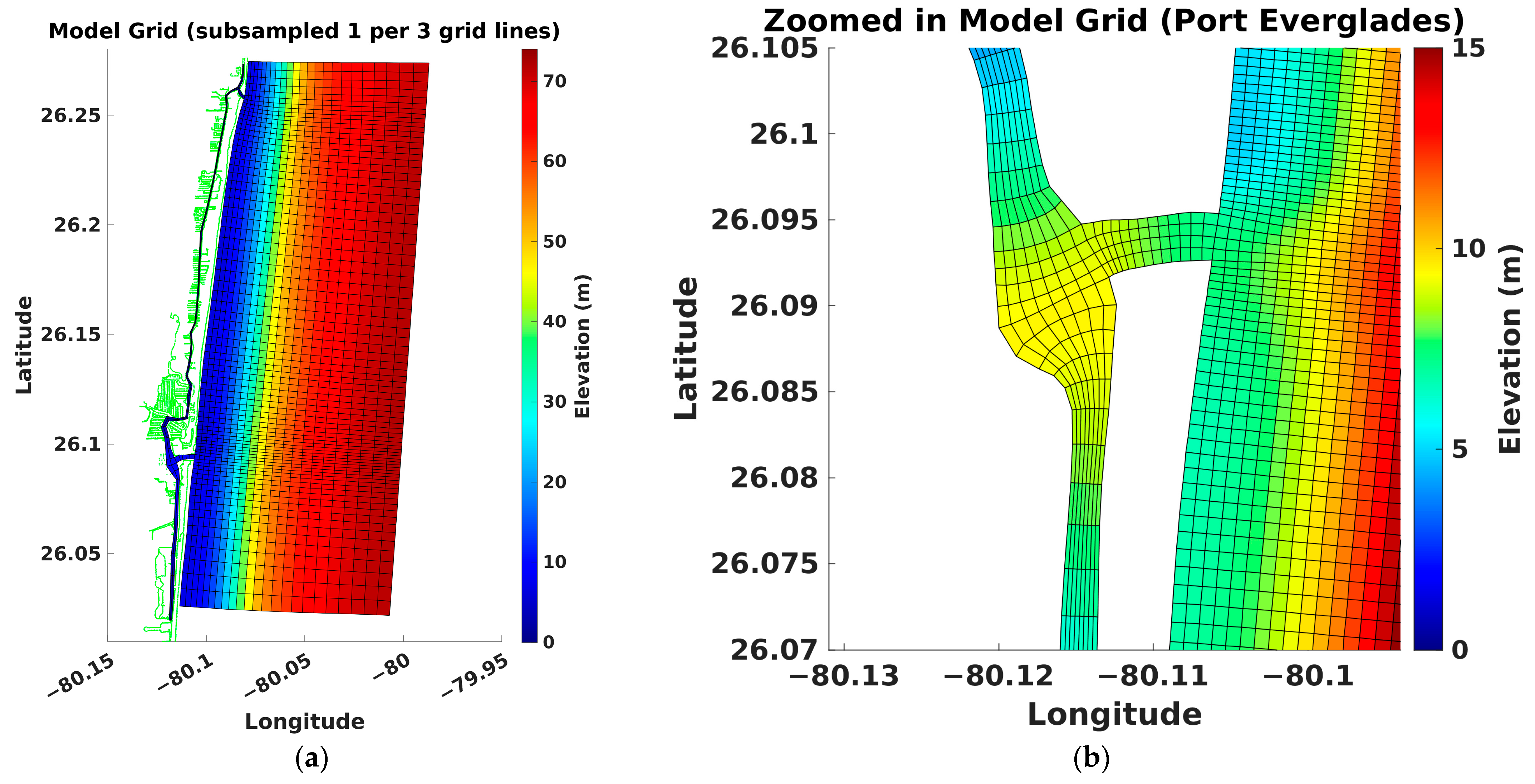
Figure 2. Mesh: (a) model grid (subsampled one per three grid lines) and bathymetry; (b) a detailed grid for the Port Everglades area.
Jmse 11 01263 g002
Figure 3. Topography extracted from the NOAA digital elevation model [11].
Jmse 11 01263 g003
Figure 4. Boundary conditions: (a) time series of sea surface elevation at East1A boundary node (denoted as East1A in Figure 4b); (b) 6 boundary nodes along and 5 boundary nodes across the open ocean.
Jmse 11 01263 g004
Figure 5. Salinity and temperature profiles at the East1A boundary node (East1A node in Figure 4b).
Jmse 11 01263 g005
Figure 6. Meteorological forcings: (a) time series of the uniformly applied U (top panel) and V (bottom panel) components of wind (location is diamond-shaped green marker in Figure 6b); (b) locations of meteorological forcings (diamond-shaped green marker) and NOAA station located in South Port Everglades (star-shaped green marker).
Jmse 11 01263 g006
Figure 7. Meteorological forcings: (a) time series of uniformly applied air temperature (top panel), relative humidity (middle panel), and net radiation heat flux (bottom panel) data at the location marked by the diamond-shaped green marker in Figure 6b; (b) time series of the uniformly applied precipitation rate (top panel) and evaporation rate (bottom panel) data in the location marked by the diamond-shaped green marker in Figure 6b.
Jmse 11 01263 g007
Figure 8. Model calibration: (a) water level time series for simulations with Chezy parameters equal to 55 (red line), 80 (blue line), and 100 (black line) in the South Port Everglades (marked by star-shaped green marker in Figure 6b); (b) time series of differences between modeled and NOAA water levels for simulations with Chezy parameters equal to 55 (red line), 80 (blue circle), and 100 (black diamond) in the South Port Everglades (marked by star-shaped green marker in Figure 6b).
Jmse 11 01263 g008
Figure 9. Model calibration: (a) scattered plot of the observed and modeled water levels for a simulation with a Chezy parameter of 55 in the South Port Everglades (star-shaped green marker in Figure 6b) in February 2018; (b) scattered plot of the observed and modeled water levels for a simulation with a Chezy parameter of 100 in the South Port Everglades (star-shaped green marker in Figure 6b) in February 2018.
Jmse 11 01263 g009
Figure 10. Model calibration: (a) water level time series of the 5-layer model (red line), 10-layer model (blue line), and observations (green dots) in the South Port Everglades station (see location in Figure 6b) in February 2019; (b) time series of differences between the observed and modeled water levels for simulations with 5 vertical layers (blue diamond) and 10 vertical layers (red line) in the South Port Everglades (see location in Figure 6b).
Jmse 11 01263 g010
Figure 11. Model calibration: (a) a 3-D vertical profile of salinity for simulations with 10 sigma layers (top panel) and 5 sigma layers (bottom panel) in the South Port Everglades (see location in Figure 6b); (b) a 3-D vertical profile of water temperatures for simulations with 10 sigma layers (top panel) and 5 sigma layers (bottom panel) in the South Port Everglades (see location in Figure 6b).
Jmse 11 01263 g011
Figure 12. Model calibration: (a) a 3-D vertical profile of the U component of horizontal velocity for simulations with 10 sigma layers (top panel) and 5 sigma layers (bottom panel) in the South Port Everglades (see location in Figure 6b); (b) a 3-D vertical profile of the V component of horizontal velocity for simulation with 10 sigma layers (top panel) and 5 sigma layers (bottom panel) in the South Port Everglades (see location in Figure 6b).
Jmse 11 01263 g012
Figure 13. Model calibration: (a) water level time series of the 2-D wind model (green line), the 1-D wind model (blue line), and observations (red dots) in the South Port Everglades station (see location in Figure 6b) in May 2018; (b) time series of differences between observed and modeled water levels for simulations with 1-D wind (blue diamond) and 2-D wind (red line) in the South Port Everglades (see location in Figure 6b).
Jmse 11 01263 g013
Figure 14. Model calibration: (a) a 3-D vertical profile of salinity for simulations with 2-D wind (top panel) and 1-D wind (bottom panel) in the South Port Everglades (see location in Figure 6b); (b) a 3-D vertical profile of water temperatures for simulations with 2-D wind (top panel) and 1-D wind (bottom panel) in the South Port Everglades (see location in Figure 6b).
Jmse 11 01263 g014
Figure 15. Model calibration: (a) a 3-D vertical profile of the U component of horizontal velocity for simulations with 2-D wind (top panel) and 1-D wind (bottom panel) in the South Port Everglades (see location in Figure 6b); (b) a 3-D vertical profile of the V component of horizontal velocity for simulations with 2-D wind (top panel) and 1-D wind (bottom panel) in the South Port Everglades (see location in Figure 6b).
Jmse 11 01263 g015
Figure 16. Model calibration: (a) water level time series for the model with the HYCOM data (blue line), ADCIRC data (green line), and observed data (red dots) at the South Port Everglades station (see location in Figure 6b); (b) differences between the observed and modeled water levels for simulations with HYCOM data (red line) and ADCIRC data (green circles) in the South Port Everglades (see location in Figure 6b).
Jmse 11 01263 g016
Figure 17. Model calibration: (a) scattered plot of the observations and model run with the ADCIRC model data in the South Port Everglades (see location in Figure 6b) in February 2018; (b) scattered plot of the observations and model run with the HYCOM data in the South Port Everglades (see location in Figure 6b) in February 2018.
Jmse 11 01263 g017
Figure 18. Model performance: (a) time series of the modeled water level (blue line) and observed data (red line) in the South Port Everglades (see location in Figure 6b) in 2018; (b) scattered plot of the modeled and observed water levels at the South Port Everglades station (see location in Figure 6b).
Jmse 11 01263 g018
Figure 19. Vertical profiles of water temperature (top panel) and salinity (bottom panel) in the South Port Everglades (see location in Figure 6b) for the year 2018.
Jmse 11 01263 g019
Figure 20. Model performance: (a) time series of NOAA (red line) and model-simulated (green line) tide data in the South Port Everglades (see location in Figure 6b); (b) time series of the differences between the observed and modeled water level (top panel), and the differences between the observed and modeled tide data in the South Port Everglades (see location in Figure 6b).
Jmse 11 01263 g020
Figure 21. Model performance: (a) modeled surface salinity (color) and currents (arrow) during the ebb tide near the Port Everglades inlet; (b) modeled surface salinity (color) and currents (arrow) during the flood tide near the Port Everglades inlet.
Jmse 11 01263 g021
Figure 22. A transect line (scattered black diamond shapes) has been drawn across Port Everglades inlet from the inlet entrance into coastal area to the end of the port into harbor. Vertical profiles of salinity, temperature, and u and v components of horizontal velocity during flood and ebb tide phases have been plotted along this transect line.
Jmse 11 01263 g022
Figure 23. Model performance: (a) vertical profiles of salinity (top panel) and water temperature (bottom panel) in the longitudinal direction (along the transect line in Figure 22) during an ebb tide event; (b) similar plots during a flood tide event.
Jmse 11 01263 g023
Figure 24. Model performance: (a) vertical profiles of the E-W velocity component (top panel) and N-S velocity component (bottom panel) in the longitudinal direction (along the transect line in Figure 22) during an ebb tide event; (b) similar plots during a flood tide event.
Jmse 11 01263 g024
Figure 25. Model performance: (a) scatter plots of amplitudes of modeled (blue colored) and observed (red colored) tidal constituents in the South Port Everglades (see location in Figure 6b); (b) scatter plots of phases of modeled (blue colored) and observed (red colored) tidal constituents in the South Port Everglades (see location in Figure 6b).
Jmse 11 01263 g025
Figure 26. Model performance: (a) time series of filtered water levels for modeled (blue line) and observed (red line) data in the South Port Everglades (see location in Figure 6b) and HYCOM data (green line); the HYCOM data point is the closest HYCOM node from Port Everglades inlet; (b) time series of the differences between modeled and observed filtered water levels (blue line) and differences between modeled and HYCOM filtered water level data (red line).
Jmse 11 01263 g026
Figure 27. Flow chart of the algorithm for automation.
Jmse 11 01263 g027
Figure 28. Flow chart of the scripting for automation.
Jmse 11 01263 g028
Table 1. Data sources.
DataSource NameURLResolution
Water level, salinity, and temperatureHYCOMhttps://www.hycom.org (accessed on 24 March 2023)0.040
Evaporation, radiation heat flux, relative humidity, air temperature, u, and v comp of wind (hindcast)NARRhttps://psl.noaa.gov/data/gridded/data.narr.html (accessed on 6 December 2020)32 km
Topography NCEI NOAA https://www.ncei.noaa.gov (accessed on 25 April 2018) 0.0055560
Radiation heat flux, relative humidity, air temperature, u, and v comp of wind
(forecast data)
NAMhttps://ftp.ncep.noaa.gov/data/nccf/com/nam/prod/ (accessed on 24 March 2023) 12 km
Water level and harmonic constituentsNOAA BUOYhttps://tidesandcurrents.noaa.gov/stationhome.html?id=8722956 (accessed on 5 June 2018) Time series
Disclaimer/Publisher’s Note: The statements, opinions and data contained in all publications are solely those of the individual author(s) and contributor(s) and not of MDPI and/or the editor(s). MDPI and/or the editor(s) disclaim responsibility for any injury to people or property resulting from any ideas, methods, instructions or products referred to in the content.