Estimation of Seawater Hydrophysical Characteristics from Thermistor Strings and CTD Data in the Sea of Japan Shelf Zone

Abstract

The knowledge of salinity in a specific sea area with high accuracy is required to solve several acoustic and hydrophysical problems on the ocean shelf. Unlike temperature, which can be measured continuously for a long time, with, for example, thermistor strings (thermostrings), salinity values of required accuracy can be obtained only using CTD profiling. This is why methods of estimating salinity from temperature could be helpful. In this paper, the authors propose using the regression method for solving this type of problem and demonstrate the efficiency of this method using examples of temperature measurements from anchored thermostrings. For the correct construction of regressions, the authors analyzed the errors of CTD measurements and suggested a method for the dynamic correction of raw CTD data. From CTD profiling datasets of 12 years (2011–2022), after their dynamic correction, the authors obtained regression polynomial formulas for calculating salinity from temperature and studied data stability in space and time at the hydrophysical test site, located in the shelf zone of the Sea of Japan. The authors consider this method efficient and applicable in solving a variety of acoustic and hydrophysical problems.

1. Introduction

The most important thermodynamic parameters of seawater are temperature, salinity, and pressure. Consequently, all hydrophysical fields in the ocean can be calculated from the spatial distribution of these parameters.

Unlike temperature (T), available data on salinity (s) in the World Ocean are irregular and inhomogeneous. Expendable bathythermographs (XBTs) are actively used to measure ocean temperature alongside ship-based, satellite, and drifter observations. XBTs are often used for routine temperature measurements from merchant and passenger ships [1,2]. Salinity data are replenished only from specialized expeditions using CTD profiling [2].

In the past few decades, due to active development and subsequent application of numerical ocean circulation models, the issue of correctly specifying the initial values of T and s of the ocean, as well as proper data assimilation, has become highly relevant. Ultimately, two approaches to solving this problem were proposed. The first [1,2] is the use of mean climatic values of T and s from available databases, interpolated on the one-degree grid. The second approach [2,3,4] is the development of methods that allow, with the availability of temperature measurements, to estimate salinity at any point in the ocean based on the statistical relationship between T and s. This approach appears more attractive because it can give a more accurate and uniform distribution of T and s data over the ocean area under study. The beginning of research on statistical dependencies of T and s goes back to the works of the first researchers—Shtokman, Stommel, and Mamayev. In the works of these authors, the theory of Ts diagrams was developed, which is based on studies of the specific patterns of combined change in temperature and salinity with depth [5,6]. They proposed using the statistical interrelation between T and s based on using the average salinity at a given temperature according to Ts diagrams [7]. Stommel proposed a solution to the problem only for a limited class of fairly homogeneous water masses with clearly defined Ts structure. In subsequent years, many authors proposed both various modifications of the Stommel method and new approaches based on the analysis of the statistical relationship between T and s, for example, [8,9,10]. We will not dwell here on the review and analysis of these methods, since it is beyond the scope of our proposed discussion. The current state of this problem can be found, for example, in [10]. Let us focus only upon some publications, in which the regression of T and s was used, which corresponds to the topic of this article. We shall note that the regression analysis for estimating salinity from temperature measurements was proposed in [11]. The authors used a regression, in which, in addition to the functional dependence of temperature and salinity on depth, they also considered the dependence of salinity on latitude. As predictors of the regression formulas, they chose the temperature values by the depth and salinity values on the ocean surface, i.e., actually, the regression was linear. For the selected area of the North Pacific Ocean, they were able to reduce the error in determining salinity by almost an order of magnitude. The next step in developing regression methods was the use of regression formulas with polynomials of higher orders. In [3,4], attempts were made to find suitable regression formulas for estimating salinity in the Gulf of Mexico and the area of the northwestern Atlantic. For the case of the Gulf of Mexico, the authors were able to show that using polynomials of the second degree is sufficient to achieve the specified accuracy [3]. For the Atlantic, the situation turned out to be much more complicated [4]. First, to approximate the salinity profile, it was necessary to use polynomials of up to the fourth order. Second, it turned out that the accuracy of the approximation could be significantly improved by dividing the study area into two areas and using its own polynomial regression in each area. In addition, the regression coefficients significantly depended on the specific season of the year. The authors explain the variability of the regression over space and seasons by the presence of water masses of different compositions, caused by the Labrador Current and the Gulf Stream [4]. The regression approach was further developed in the works of other authors, for example [2]. The main conclusion obtained in these works is as follows: regression gives good estimates of salinity only for the areas with quasi-homogeneous water composition. Thus, solving similar problems requires monitoring of water composition within the study area.

For several years, the authors of this paper have been conducting regular hydroacoustic [12,13] and hydrophysical studies [14,15,16] at the geophysical test site of the Pacific Ocean Institute of the Far Eastern Branch of the Russian Academy of Sciences (POI FEB RAS), located in the shelf zone of the Sea of Japan. The main objectives of these studies are the research of intense internal waves (IWs), the effect of background (linear) and nonlinear IWs on the formation of sound fields, and statistical evaluation of weak sound signals against the background of ambient noise, for example [12,14,15,17]. The main measuring hydrophysical instruments for the experiments were current meters, thermistor strings (thermostrings) and CTD profilers, and various hydroacoustic equipment [13,18]. To successfully solve these problems in individual points of the test site, it was necessary to obtain continuous time series of not only temperature but also salinity with an accuracy of 0.1–0.2 psu (these values will be explained below). This was the main motivation for studying the functional relationship between T and s.

The purposes of the paper are to obtain polynomial regression formulas, based on CTD data, for calculating salinity from temperature and electrical conductivity after their dynamic correction; to study the stability of the obtained regressions over the space of the test site by seasons. We also aim to determine which hydrometeorological events may change the previously obtained regression; to apply functional relationships of temperature and salinity, obtained from CTD measurements at the marine test site, for continuous calculation of hydrophysical parameters with specified accuracy from long-term thermostrings data.

The paper consists of the following sections:

In Section 2, we present a geographical description of the marine test site. Points of CTD measurements and thermostrings’ installations are specified. A general discussion of experimental data by season is included. In Section 3, CTD data errors are discussed. Methods and approaches are proposed for correcting dynamic errors, which make the greatest contribution to the process of CTD measurements under conditions of sharp temperature gradients. In this section, we present the results of the application of the authors’ methods, and the results of their comparison with the methods offered by profiler manufacturers. In Section 4, Polynomial Ts regressions, built after the dynamic correction of CTD data, for 12 years by seasons are presented. Estimates of the error obtained for calculating salinity from temperature are given. The issues of regression stability over time and space of the marine test site are discussed. In Section 5, we present two examples of using thermostrings over a long period of time and regression obtained from occasional CTD measurements and dynamic correction: the study of the buoyancy frequency and sound velocity fluctuations variability over time. In Section 6, the results of experimental studies are discussed and summarized.

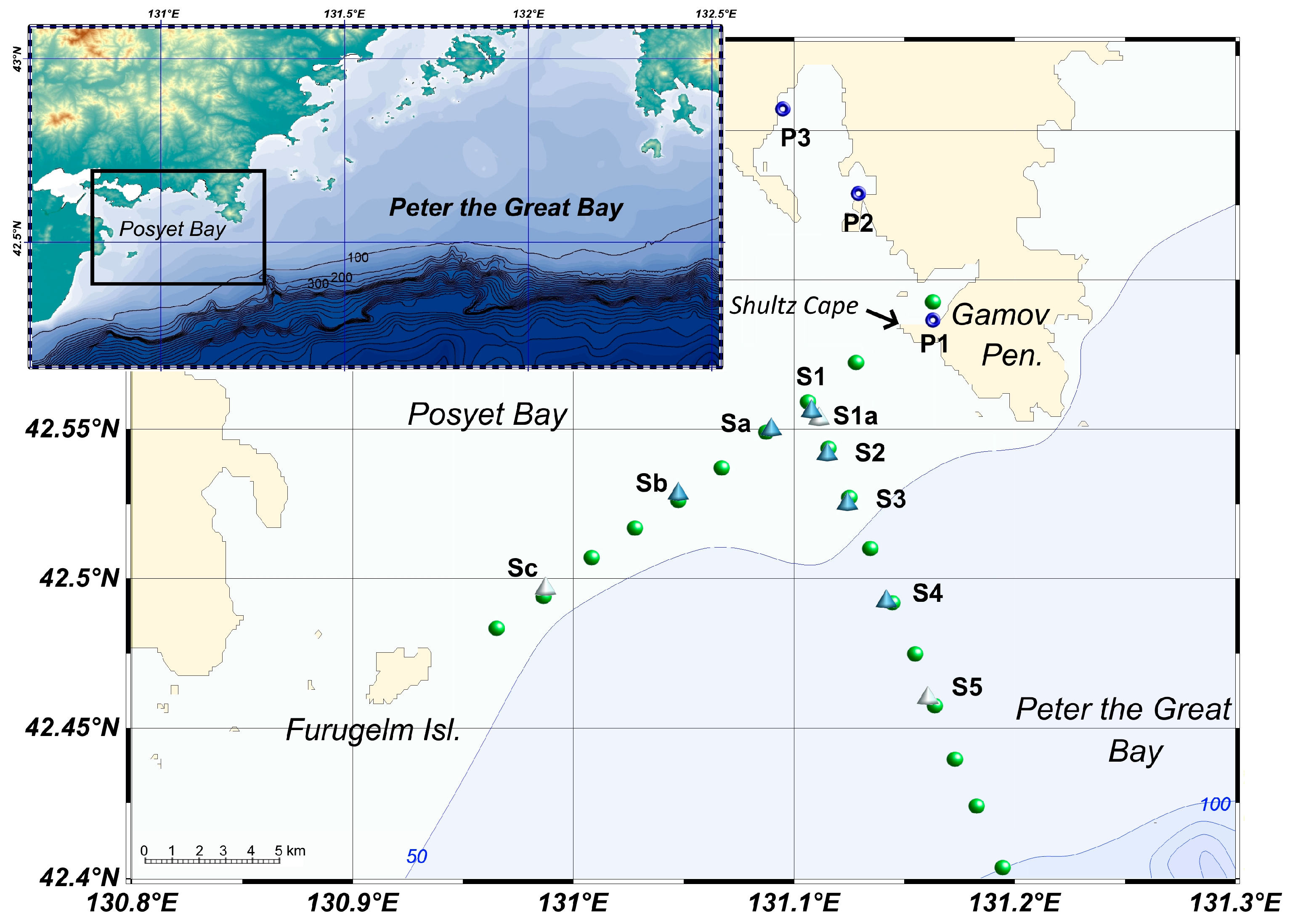
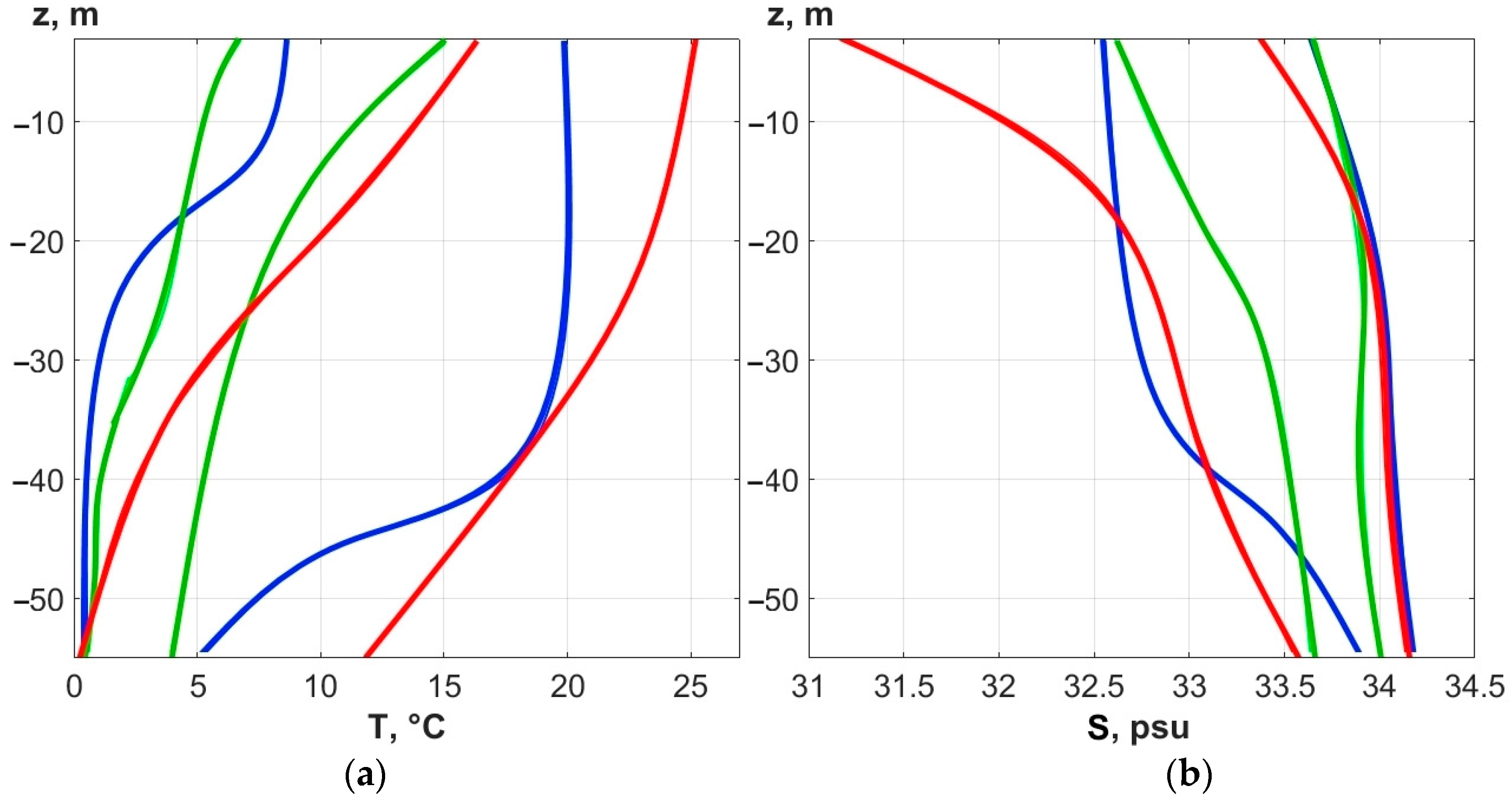
2. Study Area and Experimental Data

The experimental studies presented below were carried out at the hydrophysical test site of POI FEB RAS, located in the southwestern part of Peter the Great Bay of the Sea of Japan, including a significant part of the Posyet Bay shelf, all the way to the shelf break (to the 100 m isobath). Figure 1 shows in detail the marine part of the test site and presents a scheme of equipment setup and CTD profiling points during 2011–2022, in three seasons—spring, summer, and autumn.

In the insert to Figure 1, the area of the hydrophysical test site is marked with a rectangle. Letters S with numbers indicate thermostrings, and blue circles and letters P indicate the places of bottom hydrostatic pressure loggers’ location.

This area of the sea is characterized by a rather narrow shelf, from 10 to 25 km wide. The shelf topography in this study area is characterized by a relatively smooth change in depth up to the 100-m isobath—5 m/km, from the 100-m to 200-m isobath—20 m/km, and then an abrupt drop in the depth of 210 m/km in the depth range from 200 m to 2 km [19].

The directions of the CTD profiling routes and thermostrings setup were chosen approximately parallel (line S1–Sc) and normal (line S1–S5) to the movement of the tidal IWs fronts, which are formed at the edge of the shelf break under the action of hydrodynamic jump following the tide [20].

Various dynamic processes are possible at the test site both in the water mass and in the adjacent airspace: in spring and summer, southerly winds can cause a significant wind-induced setup from the open part of the Sea of Japan; in autumn upwelling is formed under the action of northwesterly winds; in the second half of summer and early autumn, powerful typhoons sometimes pass, with abundant precipitation [16,21]. In the southwestern direction, at a distance of about 30 km from the test site, there is the mouth of the full-flowing Tumannaya River, from the same direction, more seawards, the warm Tsushima Current flows, and from the northeast, cold waters of the Primorsky Current enter Posyet Bay. The multidirectional character of sea currents, irregularity of the river flow, and heterogeneity of the bottom topography and coastline contribute to the formation of mesoscale vortices [22,23]. Vortices, upwelling, strong winds, and typhoons can lead to active mixing, freshening of the waters in the bay, and advection of extraneous water masses. Within the framework of this paper, we will refer to any of the listed dynamic processes as a hydrometeorological event (HE). The onset of any of the listed HEs can significantly change the structure of the test site waters, formed before the HE. For this reason, noticeable changes in the thermohaline stratification of the water column of the bay can occur over time intervals of the order of the synoptic scale. Figure 2 shows the ranges of temperature changes according to CTD profiling at the stations of the hydrophysical test site for 12 years. Here, the left line of one color shows the minimum and the right line of the same color shows the maximum values of temperature and salinity in a certain season. Observations within one season averaged 2 weeks. The temperature range for all seasons for the period of 2011–2022 was from 0 to 26 °C, and the salinity changes range was from 31.2 to 34.1 psu.

Figure 3 shows the characteristic temperature distributions recorded by the S4 thermostring in different seasons: 24 May–7 June 2022 (331 h), 31 July–14 August 2022 (336 h), and 3–14 October 2022 (257 h).

Figure 3 (top) illustrates the spring dynamics of temperature stratification caused not only by radiative heating of the upper layer but also by the advection of relatively warm waters from the open part of the Sea of Japan into the shelf zone of the bay under the influence of the southern monsoon. The temperature distribution along z is predominantly linear 0.1 °C/m with thin gradient layers of up to 1 °C/m, in the absence of a stable upper homogeneous layer.

Figure 3 (middle) shows a typical example of summer thermal stratification of the water column of the bay when the period of intense radiative heating ends and the temperature of the surface layer increases to 24–26 °C. At the same time, low temperatures of up to 1 °C remain in the bottom layer due to the inflow of cold waters from the open part of the Sea of Japan, also due to tidal processes and the Primorsky Current. Due to intense heating, temperature gradients of up to 3 °C/m and more are formed in the upper layer at horizons of up to 6–10 m. Below, there is a low-gradient layer of 0–0.2 °C/m, covering the main water column to 40–45 m. The near-bottom high-gradient layer of 1–4 °C/m is formed under the influence of the dynamic processes described above.

Figure 3 (bottom) shows typical autumn temperature stratification, when, due to cooling under the influence of the northern monsoon, a characteristic three-layer structure is formed with pronounced homogeneous layers 10–15 m thick in the upper and lower parts and an intermediate thermocline layer with a gradient of up to 2.5 °C/m. In the case under consideration, during the observation period from 3 October to 14 October 2022, the thermocline changed its thickness two-fold and the position of the upper boundary—by 20 m.

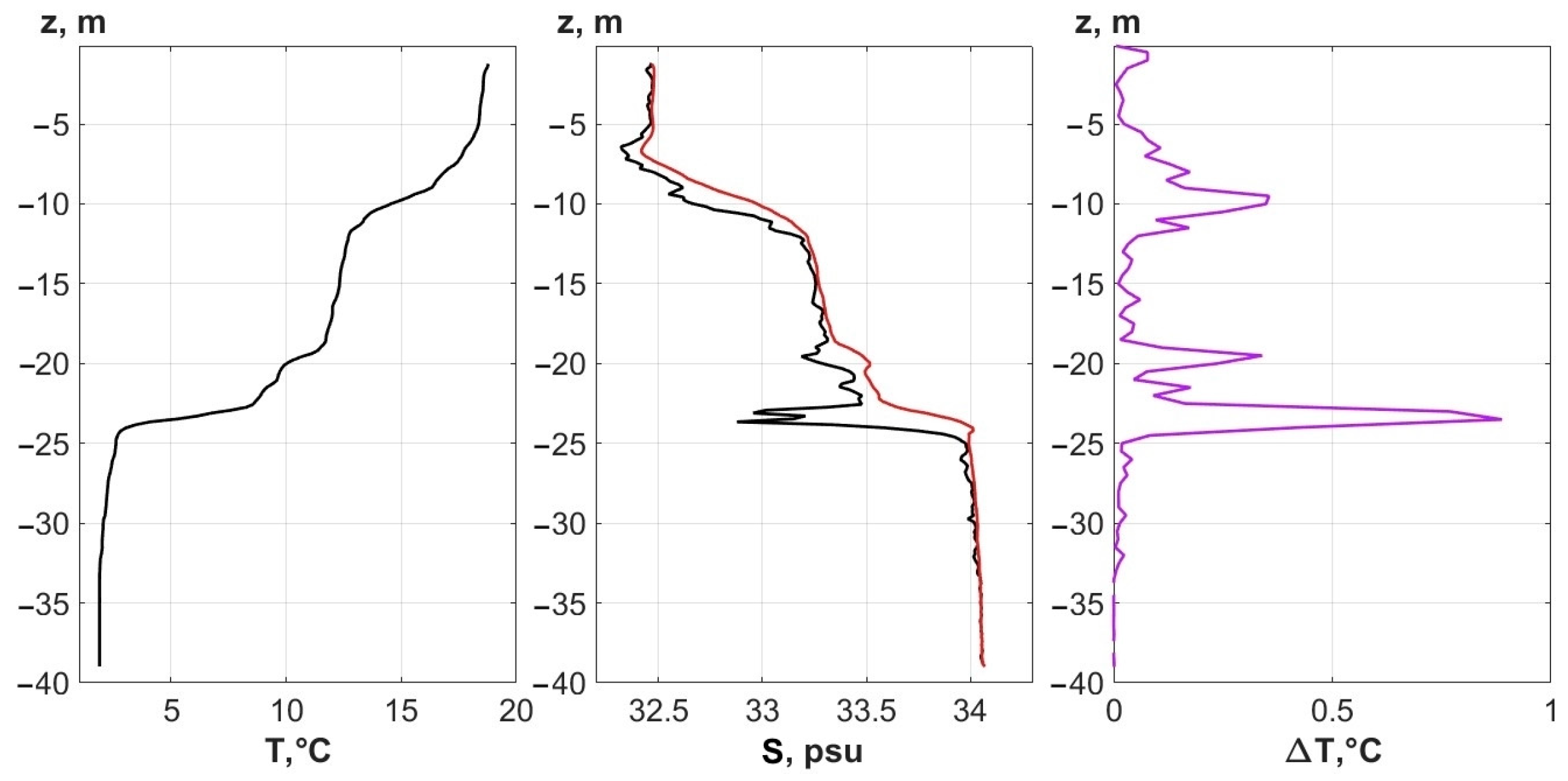
3. Correction of CTD Data

We should note that in the past few decades, manufacturers of CTD profilers have equipped them with high-precision modern sensors for temperature, electrical conductivity, and pressure [24,25]. An inexperienced researcher may hope that the characteristics of the sensors are more than sufficient for direct measurement of hydrophysical fields with the required accuracy. Indeed, in several oceanological problems, one can limit oneself to directly measured primary parameters T₁, E₁, and p₁ (temperature, electrical conductivity, and pressure), which are then used to calculate derived parameters, for example, s₁, c₁, ρ₁, and N₁ (salinity, sound speed, density, and buoyancy frequency). This is so if we limit ourselves to the analysis of distributions of hydrological parameters of water in the absence of sharp gradients to monitor the dynamics of internal waves. For experimental and model studies of low-frequency sound, the primary values of the sound speed may also be sufficient. However, this is not always the case. The presence of high-temperature gradients in the thermocline layers can significantly “noise” the derived parameters of CTD profiling [26]. This problem is especially important in the shelf zone. Here, the layer of seasonal thermocline can occupy a significant part of the water column. Thus, the errors in the CTD profiling data in shallow seas will be much greater than in deep oceans [27].

In the process of working with data from many years, the authors established that the problem of correcting CTD data is especially important for the proper construction of Ts regression curves. Dynamic errors of CTD measurements in shallow seas, as a rule, lead to incorrect construction of such regressions [28,29].

3.1. Errors of CTD Measurements

Over the past 12 years, we performed CTD measurements with SBE 19plus profilers (Sea-Bird Electronics, Inc., Bellevue, WA, USA), and with RBR XR-620, XRX-620, RBRconcerto (Ricard Brancker Research Ltd., Toronto, ON, Canada) models with similar characteristics.

Marine environment parameters measured with profilers contain instrumental and methodological errors. The methodological errors in CTD data are due to measurement methods and related conditions. In particular, with the drift and pitching of the vessel, due to the mechanical connection of the winch (using a cable) with the submersible CTD profiler, the mode of the device movement is unsteady. In a stratified environment, CTD profiling data will contain distortions comparable to estimates of dynamic errors [30]. Instrumental errors consist of three parts—systematic, random, and dynamic. All these errors are determined by the metrological characteristics of the CTD profilers, and by stratification of the studied water column [31]. The metrological characteristics of the profilers are usually given by the manufacturers in the provided manuals [24,25]. For example, for the XR-620 profiler, the accuracy of measuring electrical conductivity, temperature, and pressure is 0.003 mS/cm, 0.002 °C, and 0.4 kPa, respectively. The resolution of all three sensors is 0.001 mS/cm, 0.00005 °C, and 0.005 kPa, respectively. RBR estimates the inertia of the thermometer as 0.1 s, and that of the pressure sensor—as 0.01 s. For the electrical conductivity sensor, inertia is a function of the speed of the profiler movement. The other profilers mentioned above have similar metrological characteristics.

Analysis of the measured data and its further use for solving several hydrophysical problems is impossible without assessing and taking into account the levels of errors, and primary data processing. Both procedures allow the reduction of the contribution of these errors to the required level. The systematic component of instrumental error depends on the accuracy of determining the calibration coefficients established in the laboratory during the calibration of the corresponding sensitive element (sensor) of the instrument. Evaluation of the level of this component takes into account the accuracy and drift values declared by the manufacturer [24,25]. The random component of instrumental error includes the noise that occurs in the measuring channel of the sensor, and the capacity of the used ADC, i.e., signal quantization step. Estimates of this type of error in the data of most modern hydrological instruments, as a rule, do not exceed 2–3 quantization steps [27].

The errors in the measured values of temperature T₁ and electrical conductivity E₁ affect the subsequent calculations of other hydrophysical parameters of water, which are determined by the values of temperature, salinity, and pressure η = η(T, s, p). To estimate such an effect on salinity s(T, E, p), density ρ(T, s, p), and sound speed c(T, s, p) of water, we will use linearized phenomenological formulas [32]:

$$\begin{array}{l}{s}_1=s\left(T,E,p\right)+\frac{\partial s}{\partial T} \delta T+\frac{\partial s}{\partial E}\delta E+\frac{\partial s}{\partial p}\delta p,\\ {\eta }_1=\eta \left(T,s,p\right)+\frac{\partial \eta }{\partial T} \delta T+\frac{\partial \eta }{\partial s}\delta s+\frac{\partial \eta }{\partial p}\delta p, \eta =\left\{\rho , c\right\}\end{array}$$

(1)

where δT = T₁ − T, δE = E₁ − E, δs = s₁ − s, and δp = p₁ − p.

Table 1. Values of the coefficients of the equations for determining the errors in s, ρ, c.

∂s/∂T = 0.6–1.3 psu/°C	∂ρ/∂T = −0.3–0 [g/cm3]/°C	∂c/∂T = 2.6–4.4 [m/s]/°C
∂s/∂E = 0.7–1.3 psu/[mS/cm]	∂ρ/∂s = 0.7–0.8 [g/cm3]/psu	∂c/∂s = 1–1.3 [m/s]/psu
∂s/∂p = 0.0005 psu/dbar	∂ρ/∂p = 0.0046 [g/cm3]/dbar	∂c/∂p = 0.016 [m/s]/dbar

shows values of the coefficients of the linearized equations calculated for the following ranges of parameters T, E, p, s: 1 ≤ T ≤ 25 °C, 27 ≤ E ≤ 51 mS/cm, p ≤ 200 dbar, 31 ≤ s ≤ 34 psu. The boundaries of the parameter variation ranges were chosen based on the analysis of CTD profiling data from 2011 to 2022.

If we assume that systematic and random errors of the measured parameters of the state and electrical conductivity are independent, then the errors of the calculated parameters, for example, speed of sound Δc₁ can be estimated as follows:

$$\Delta c_1={\left[{\left(\partial c/\partial T \Delta T\right)}^2+{\left(\partial c/\partial s \Delta s\right)}^2+{\left(\partial c/\partial p \Delta p\right)}^2\right]}^{1/2}.$$

(2)

As we know, the largest values of instrumental errors in CTD profiling data fall on their dynamic components, which significantly depend on the stratification of seawater, the inertia of the CTD profiler sensors, and the mode of its movement in the water column [28,33]. In many in-situ measurements, dynamic errors can exceed all other instrumental errors by dozens of times [27].

Influence of inertial effects on the measured values of electrical conductivity E₁(t) and temperature T₁(t) in stratified layers of seawater E(t) and T(t) at any moment of time t are described by approximated first-order differential equations [31]:

$$T\left(t\right)=T_1\left(t\right)+{\tau }_T\frac{d}{dt} T_1\left(t\right), E\left(t\right)=E_1\left(t\right)+{\tau }_E\frac{d}{dt} E_1\left(t\right),$$

(3)

where the values of the inertial coefficients ${\tau }_T$ and ${\tau }_E$ can change over time and depend on the structural features, on properties of the sensitive elements of temperature and electrical conductivity sensors materials, and also they significantly depend on parameters of the flows surrounding the sensors during movement of the CTD profiler [33]. From Equation (1) it follows that the dynamic errors are proportional to the values of the derivatives $T_1^{\prime }, E_1^{\prime } \left(T^{\prime }\equiv dT/dt\right)$:

$$\Delta T_1\left(t\right)=T\left(t\right)-T_1\left(t\right)={\tau }_T T_1^{\prime }\left(t\right), \Delta E_1\left(t\right)={\tau }_E E_1^{\prime }\left(t\right).$$

(4)

Sensors of the SBE 19plus profiler—a thermometer and an SBE 4 conductivity cell are connected to the pumping channel of the SBE 5 pump. Due to the constant velocity of the measured fluid inside the channel, the values of the inertial coefficients are estimated by constants τ_E(t) ≈ 0.06 s and τ_T(t) ≥ 0.5 s [24,34].

The XR-620 and XRX-620 profilers are equipped with an induction cell of conductivity and a fast-response platinum thermometer [25], which, when the device moves in the water column, is freely washed by the oncoming flow of seawater. In this case, the inertial coefficients depend on the profiling velocity v. With stationary motion of the device, v(t) = const, and laminar modes of flow around the sensors, these dependences have the form: τ_E(v) ~ v^−1.5 and τ_T(v) ~ v^−0.5 [28].

The authors took into account the possible limits of the variability of the inertial coefficients and all profiling was performed at the speed of 0.5 < v < 1.5 m/s. Under such conditions, the expected inertia of the XR-620 profiler thermometer does not exceed τ_T(v) ≤ 0.2 s, and the time constant of the induction cell is minor, τ_E(v) << τ_T(v), and can be neglected [28].

As we have noted above, the shelf zone of Peter the Great Bay from May to October is characterized by a developed seasonal thermocline. Its structure contains layers with significant temperature gradients |∂T/∂z| ~ 1–3 °C/m. In these layers, the dynamic errors of temperature measurement with the SBE 19plus and XR-620 profilers are dozens of times greater than the total levels of systematic and random components.

Table 2. Systematic, random, and dynamic errors (|∂T/∂z| = 1 °C/m).

CTD Profiler	Seawater Parameters	Random Errors	Dynamic Errors
SBE 19plus	T	0.007 °C	0.5 °C
	s	0.012 psu	0.5 psu
	ρ	10−5 g/cm3	40 × 10−5 g/cm3
	c	0.03 m/s	2 m/s
RBR XR-620	T	0.004 °C	0.2 °C
	s	0.008 psu	0.5 psu
	ρ	0.6 × 10−5 g/cm3	20 × 10−5 g/cm3
	c	0.015 m/s	1 m/s

presents estimates of various types of errors for two types of CTD profilers. Systematic and random errors are calculated based on the data provided by the manufacturers, taking into account formulas (1) and (2) and the data in Table 1 [24,25]. Dynamic errors are estimated here under the assumption that profiling was carried out in a thermocline with temperature gradient |∂T/∂z| = 1 °C/m with profiler movement speed v = 1 m/s. At such speed, the temporal temperature variability in the sensor point is |∂T/∂t| = 1 °C/s, which makes it possible to estimate the errors in temperature and electrical conductivity, taking into account Equation (4). Other hydrophysical parameters are estimated with account for Formula (1) and data from Table 1.

3.2. Minimization of Dynamic Errors

As it follows from Table 2, dynamic errors are an order of magnitude greater than systematic and random errors. For many tasks, this situation can be unacceptable. For example, if we study fluctuations in the speed of sound on the shelf, then we must ensure accuracy no worse than 0.1–0.2 m/s, because the magnitude of these fluctuations can be 1–4 m/s [35]. If sound speed fluctuations are obtained from temperature based on the regression Ts curve, then the requirements for measurement accuracy will only increase.

Next, we shall define possible methods of correcting CTD data and propose algorithms for minimizing dynamic errors.

Let us first consider the simplest situation, when salinity in seawater is constant s(z) = s₀, and temperature distribution along the vertical line is described by the harmonic function

$$T(z)=T_0+\theta \exp \left(2\pi i z/L\right),$$

(5)

where L is the scale of temperature variability relative to the value of temperature T₀, and θ is the amplitude of these variations. With sufficiently small linear dimensions of temperature and electrical conductivity sensors, according to Equation (1), they are inertial links of the first order and correspond to the characteristics of linear converters with lumped parameters. Let further ω = 2πv/L be a fixed value of frequency; v is the speed of the profiler. Then measured profiles T₁(t) and E₁(t) are determined by the following equations:

$$\begin{array}{l}{T}_1\left(t\right)=T_0+\theta a_T \exp \left[i\omega \left(t+{\phi }_T\right)\right],\\ E_1\left(t\right)=E_0+\partial E/\partial T \theta a_E \exp \left[i\omega \left(t+{\phi }_E\right)\right]+\partial E/\partial p p(t),\end{array}$$

(6)

were $\phi ={\omega }^{-1} \psi$, and $a={\left(1+{\omega }^2{\tau }^2\right)}^{-0.5}, \psi =\mathrm{arctg}\left(\omega \tau \right)$ are amplitude and phase functions of the corresponding sensors.

Lack of equality of inertial coefficients τ_T ≠ τ_E leads to a mismatch between the profiles T₁(t) and E₁(t) in terms of amplitudes a_T ≠ a_E and phases φ_T ≠ φ_E. Inside the temperature gradient layer, this mismatch manifests itself as a phase shift Δφ = φ_E − φ_T between the derivatives and $T_1^{\prime }$ and $E_1^{\prime }$, and in the measured salinity profile additional parasitic changes appear, called “salinity spike” [36]

$$\Delta s_1=\partial s/\partial T \theta a_E \left[1-a_T/a_E \exp \left(i\omega \Delta \phi \right)\right] \exp \left[i\omega \left(t+{\phi }_E\right)\right].$$

(7)

The simplest analysis of frequency functions shows that with small-scale variations L→0 (ω→∞) in Equations (6) and (7) influence of the amplitude function a→0 (φ→0) prevails. As the scale L→∞ (ω→0) increases, the contribution to Equations (6) and (7) of the phase component φ→τ (a→1) increases. At stratification scales L ≥ 20 vτ, the estimates a ≥ 0.95 and φ ≈ τ are valid, and the contribution of the amplitude function can be neglected when estimating the dynamic error of the water environment parameters [27,36].

In real conditions, stratification of the seawater column usually has a stepped structure, with an alternation of quasi-homogeneous and gradient layers. Assuming a layer thickness of Δz, we consider the scaling parameter L = 2Δz. CTD data measured in gradient layers with a thickness of Δz ≥ 10 vτ_E, under the condition of τ_T > τ_E, contain dynamic errors, which are mainly determined by the phase functions φ_T ≈ τ_T and φ_E ≈ τ_E, since in this case a_T ≥ 0.95 and a_E ≈ 1. If the temperature T₁(t) is measured in such layers with a sufficiently high frequency of sensor polling f > 1/τ_T, then the dynamic error of temperature can be significantly reduced by shifting the temperature in time:

$$T_2\left(t\right)=T_1\left(t+n \delta t\right),$$

(8)

where the interval of sensor polling δt = 1/f and some integer n = (1, 2, 3…).

The manufacturers of SBE and RBR profilers also suggest the time shift of the measured temperature T₁(t) according to Formula (8) in their supplementary materials to the manuals [37,38]. We only note that the efficiency of method (8) is affected by the measure of the difference between the displacement parameter and the phase function |nδt − φ_T| < 0.5δt. The measured electrical conductivity E₁(t), as a rule, is not corrected by the time shift (8) due to the smallness of the value of the time constant τ_E < δt.

We will now assume that the CTD profiling process is performed at the constant speed v = const, and before the initial profiling time t = 0, the profiler was in a homogeneous water layer for some time longer than τ_T. Then, during profiling, τ_T = const, T₁(t ≤ 0) = T(0), i.e., at the initial moment t = 0, the dynamic errors were negligible. Following Equation (3), we write equations for the measured value T₁(t) in terms of the true water temperature near the moving temperature sensor T(t) in the form of an exponential low-pass filter [39,40]:

$$T_1(t)=\exp \left(-\delta t/{\tau }_T\right) T_1(t-\delta t)+\left[1-\exp \left(-\delta t/{\tau }_T\right)\right] T(t).$$

(9)

For the piecewise constant temperature T(t), Formula (9) is the exact solution to (3), and for a smooth profile T(t) it is a difference scheme for calculating T₁(t) on the time grid with step δt.

In accordance with Formula (9), we now formally define the procedure for “recovering” the true temperature T(t) from the results of measurements T₁(t):

$$T_2\left(t\right)=\left[T_1\left(t\right)-\exp \left(-\delta t/{\tau }_2\right) T_1(t-\delta t)\right]/\left[1-\exp \left(-\delta t/{\tau }_2\right)\right].$$

(10)

In the case of a hypothetical ideal CTD profiling at τ₂ = τ_T, procedure (10) leads to the complete elimination of dynamic errors T(t) = T₂(t). However, in real conditions, this is not the case for the following reasons. First, even with the equality τ₂ = τ_T, calculations using Formula (10) cannot give a good result due to the growth of random components of errors T₁. Second, under real profiling conditions, the multifactor nature of the inertial effect during temperature measurements can manifest itself [27,41]. This effect is due to the superposition of inertial processes occurring inside the thermometer and in the boundary layer surrounding its body. Using a high-order equation to describe such a superposition of effects is difficult due to the lack of reliable information about the inertia of each selected inertial link. Therefore, frequency characteristics of thermometers that are part of CTD profilers are represented by the inertial link of the 1st order with additional phase shift [42],

$$T_3\left(t\right)=T_1\left(t+n\delta t\right)+{\tau }_T T_1^{\prime }\left(t+n\delta t\right), T_3\left(t\right)\approx T\left(t\right),$$

(11)

which corresponds to the scheme “exponential recovery (10) + time shift (8)” [29,35]. Thus, the inertial coefficient of a thermometer (11) should be estimated by the sum τ₃ = τ_T + nδt. Here, the first component τ_T is the parameter of the exponential filter (9), and the second component nδt reflects the presence of an additional phase shift in the measured temperature T₁(t) with respect to the measured electrical conductivity E₁(t). Accounting for the second component using procedure (8) is possible only when processing high-resolution CTD data n >> 1 [27].

Before we finalize the scheme of dynamic data correction proposed here, and give two examples of its application, we shall, first, briefly discuss the approaches of manufacturers of SBE and RBR profilers to solving this problem.

We should note that SBE was one of the first to recommend the users of their profilers to perform dynamic correction of profiling data using a package of programs for primary data processing. Similar proposals for RBR profilers have appeared only in the last few years [38,43,44]. Since the methods of these manufacturers are quite similar, we will limit ourselves here to discussing the primary processing of CTD data by the SBE-Data Processing program, which contains several procedures, executed in sequence [37]. Here, first, the “Filter” procedure reduces levels of random measurement errors. Its numerical scheme uses the first two terms of power series expansion of the exponential low-pass filter (9). In this case, it is proposed to smooth the temperature and electrical conductivity profiles measured by SBE 19plus at equal filter parameters, τ₂ = 0.5 s. Furthermore, using the “Align” procedure, structural features of the smoothed profiles T₁(t) and E₁(t) are aligned to eliminate their dynamic (phase) mismatch and reduce the amplitudes of false emissions when determining salinity. This procedure corresponds to the time shift (8) and, at the value of the shift parameter nδt = 0.5 s, is used to correct the temperature data of SBE 19plus [37].

The electrical conductivity values, measured by the SBE profilers, contain an additional error due to the thermal contact of the studied portion of seawater with the body of the SBE 4 conductivity cell. This effect occurs when crossing temperature gradient layers and contributes to the heating/cooling of the measured portion of the liquid [34]. As a result, its electrical conductivity differs from the initial value, which also leads to errors in determining salinity [2]. Elimination of this error is carried out by the “Cell Thermal Mass” procedure.

The standard SBE 19plus data processing scheme, which includes step-by-step execution of the listed procedures, leads to a significant reduction in errors in determining salinity, but retains a noticeable dynamic error in the measured temperature. Smoothing the profile T₁(t) by filter (9) at the recommended value τ₂ = 0.5 s increases this error component, and the subsequent time shift (8) only partially reduces the total level of its phase component. As a result, the data processed by SBE-Data Processing contains a significant share of dynamic errors and can fail to meet the accuracy requirements for some tasks. For example, they may be insufficient for problems of determining small fluctuations in the speed of sound and density, and may also be unacceptable for constructing regression Ts curves.

To reduce the levels of dynamic errors in CTD data as much as possible, we will continue to use an alternative processing scheme everywhere. To do this, we replace the smoothing of the profile T₁(t) by filter (9) with the “recovery” procedure (10), preserving its equalization (8) and smoothing of the profile E₁(t) (9). In this case, we will select the optimal values of the “recovery” processing parameters τ₂, displacement nδt, and smoothing τ₃ according to the criterion of minimum dispersion of high-frequency salinity fluctuations on scales of up to 2 s [27,36].

Figure 4 and Figure 5 below show the results of data processing, obtained by the SBE 19plus and RBR XR-620 profilers at the end of August 2014 and at the beginning of September 2011. At the end of summer and beginning of autumn, due to the abundant precipitation of the wet monsoon and accumulated solar radiation, the water masses of Peter the Great Bay shelf zone were characterized by high background values of salinity and temperature gradients. Therefore, the CTD measurements performed in the above period contained the maximum levels of dynamic errors. Let us evaluate the efficiency of the standard and alternative processing schemes using CTD data, obtained by SBE 19plus in August 2014. Figure 4 shows the results of measurements performed under conditions close to ideal (speed 1.0–1.5 m/s, in the absence of waves and wind) near station S1. The profile of the measured temperature T₁(z) in Figure 4 shows a three-layer stratification of the water mass of the bay, typical for the end of the summer season. The upper and bottom layers had temperature gradients, |∂T/∂z| ≤ 0.15 °C/m, which is an order of magnitude lower than in the thermocline located between 10 and 30 m horizons, where a drop from 23 to 6 °C (|∂T/∂z| ≈ 1 °C/m) was observed. Accordingly, the levels of dynamic errors in the CTD data, obtained in these layers, also differed. Their high values in the thermocline layer contributed to a more pronounced dynamic mismatch between the measured profiles T₁(t) and E₁(t), which manifested itself as a false structure when calculating the salinity s₁(z) = s(E₁, T₁, p₁). Significant peaks on the profile s₁(z) up to 1 psu correspond to gradient interlayers of the thermocline |$T_1^{\prime }$(t)| ≤ 3 °C/s.

Processing of CTD data by the SBE-Data Processing program, performed in accordance with the attached recommendations, led to a significant reduction in false emissions when calculating s₂(z) = s(E₂, T₂, p₁) (see Figure 4). At the same time, the alternative correction scheme proposed by us, due to optimization of the matching procedure of temperature and electrical conductivity profiles T₃(t) and T₃(t), at processing parameters: τ₂ = 0.17 s, nδt = 0.25 s, and τ₃ = 0.37 s, allowed the minimization of the salinity inversions s₃(z) = s(E₃,T₃, p₁). Comparing the results of dynamic correction schemes, we have discrepancies in temperature |T₂(z) − T₃(z)| ≤ 0.5 °C and salinity |s₂(z) − s₃(z)| ≤ 0.28 psu.

For the processing scheme proposed here, the absence of false salinity structure is achieved by relative equalization of dynamic errors of the reconstructed temperature and the smoothed electrical conductivity əE/əT ΔT₃ ≈ ΔE₃. At the same time, the dynamic component of temperature error remains at a high level: ΔT₃ ≈ (τ_T +τ_E) $T_1^{\prime }$. For example, at average values of the gradient in thermocline |$T_1^{\prime }$(t)| ≈ 1 °C/s and ΔT₃ ≤ 0.5 °C repeated use of the “recovery” procedure at τ₄ = τ₂ + τ₃ almost eliminates the dynamic temperature errors; however, in this case, the random component of the error increases to 2–3 levels of the initial random error, approximately up to 0.01 °C. Thus, the temperature distribution T₃(z) obtained by correcting T₁(z) using the displacement (8) and “recovery” (10) procedures is as close as possible to the true temperature T(z) and considerably differs from T₂(z) obtained by the SBE-Data Processing. At the final stage of data processing, to reduce the levels of random errors, the function s₃(t) was filtered in the time domain by moving average with window Δt = 1s, and the profiles s₃(z) and T₃(z) were reduced to depth step Δz = 0.5 m.

Dynamic correction of the data obtained with RBR profilers (XR-620, XR-620, and RBRconcerto) was carried out according to the scheme proposed above (8)–(10). Its efficiency is demonstrated by the results presented in Figure 5. Here, for CTD profiling performed at point S2 in the absence of wind and ship motion (v = 1 m/s), the minimum possible levels of dynamic errors ΔT₃ ≤ 0.01 °C and Δs₃ ≤ 0.02 psu at optimal correction values (8)–(10) τ₂ = 0.009 s, nδt = 0.167 s, and τ₃ = 0.007 s. When calculating salinity s₃(z), almost all false emissions that reached 1 psu in s₁(z) were eliminated, and the dynamic temperature correction T₁(z) led to a decrease in T₃(z) by 0.1–1 °C in thin gradient layers.

Based on the proposed methodology of dynamic correction of CTD data and Table 1 and Table 2, some hydrophysical parameters of water were estimated for the above measurements by SBE 19plus and RBR XR-620. Error estimates have the following absolute values: |ΔT| ≤ 0.01 °C, |Δs| ≤ 0.02 psu, |Δρ| ≤ 2 × 10⁻⁵ g/cm³, and |Δc| ≤ 0.05 m/s. Let us remind ourselves that measurements were performed in the absence of ship motion at the speed v(t) = 1 m/s, and temperature gradients in both experiments were approximately up to 1 °C/m.

We shall also remark on the RBRconcerto profiler. The results of similar data processing for this profiler according to the scheme (8)–(10) do not always reveal the phase shift nδt (8) when estimating the mismatch of the measured temperature and electrical conductivity profiles. This is due to the design of this model (the thermometer is built into the conductivity sensor), and insufficiently high polling rate of 6 Hz.

In conclusion of this section, it is also worth mentioning that when processing CTD data obtained under conditions of drift and pitch and roll of the ship, as a rule, it is not possible to achieve a satisfactory reduction of the dynamic errors T₁(t) and E₁(t). Such an example of measuring temperature and electrical conductivity with the XR-620 profiler in mid-August 2011 in the presence of pitching and rolling of the ship, due to which the profiler movement velocity varied within v(t) ≈ 0.55 ± 0.25 m/s, is shown in Figure 6. As a result of the violation of the device movement dynamics, local inversions appeared in the structures of the profiles of the measured parameters. When calculating salinity s₁(z), these inversions manifested themselves as distortions not only on the pitch and roll scale, but also on large scales. The salinity profile shown in Figure 6 shows a decrease in background values of 0.05 psu in the lower gradient layer of the thermocline.

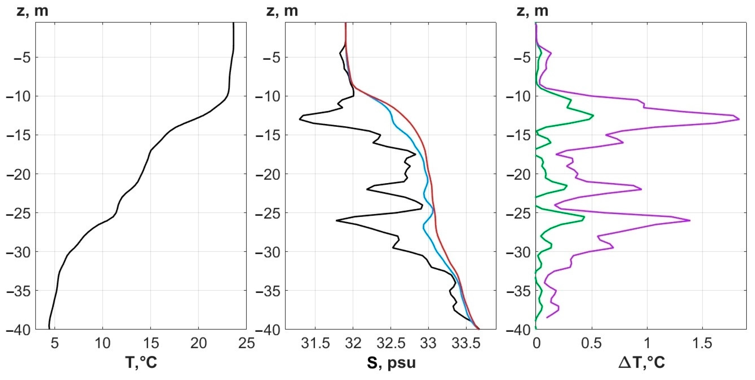
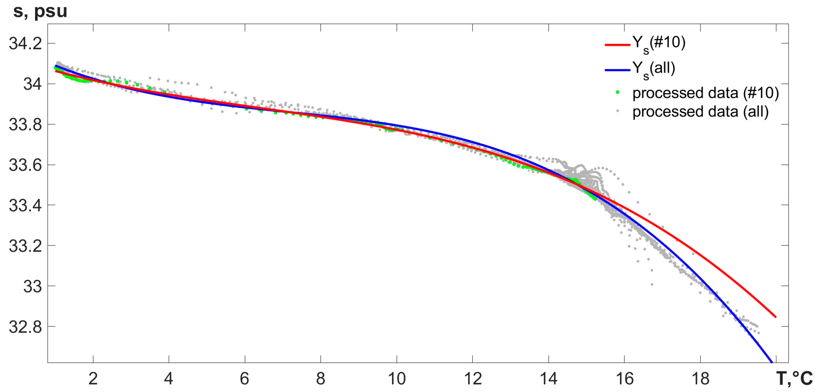
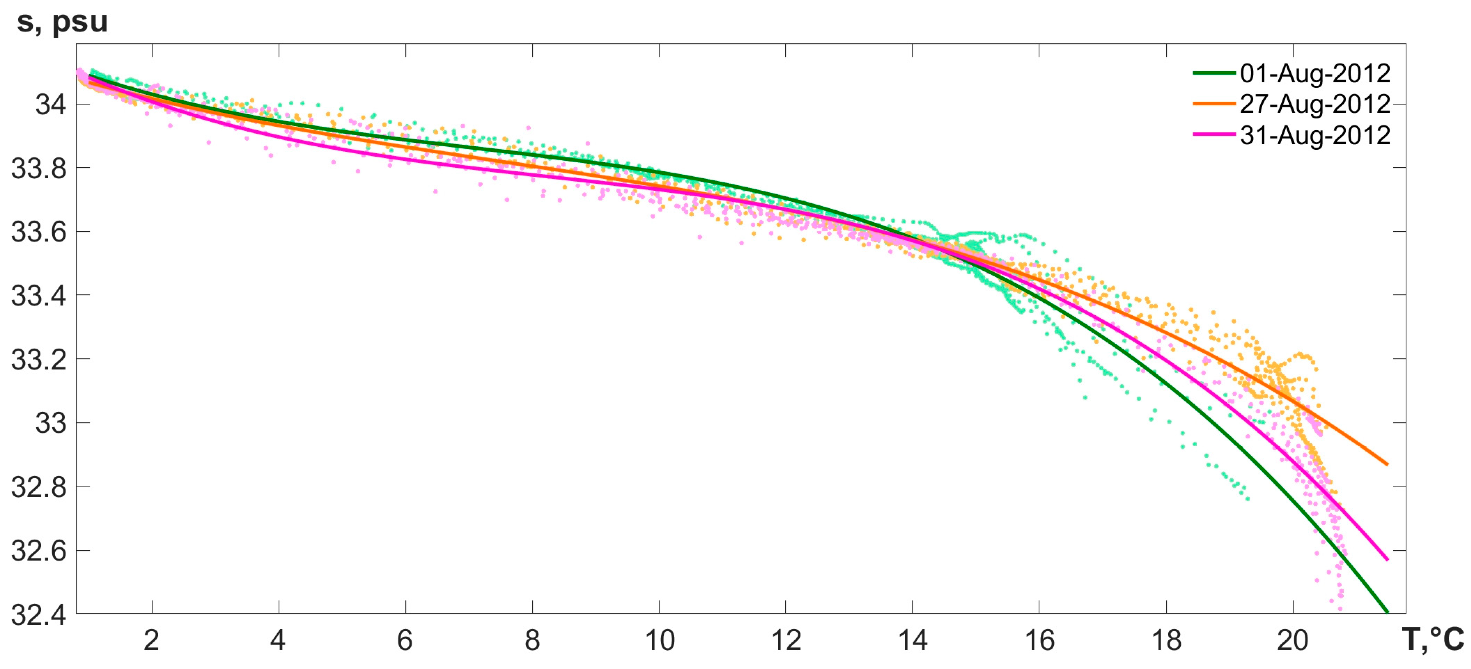
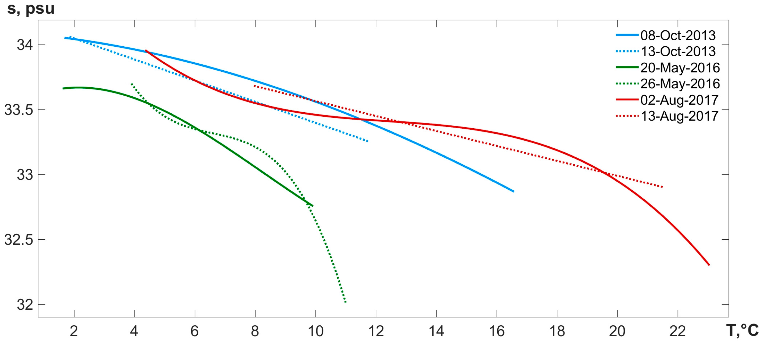
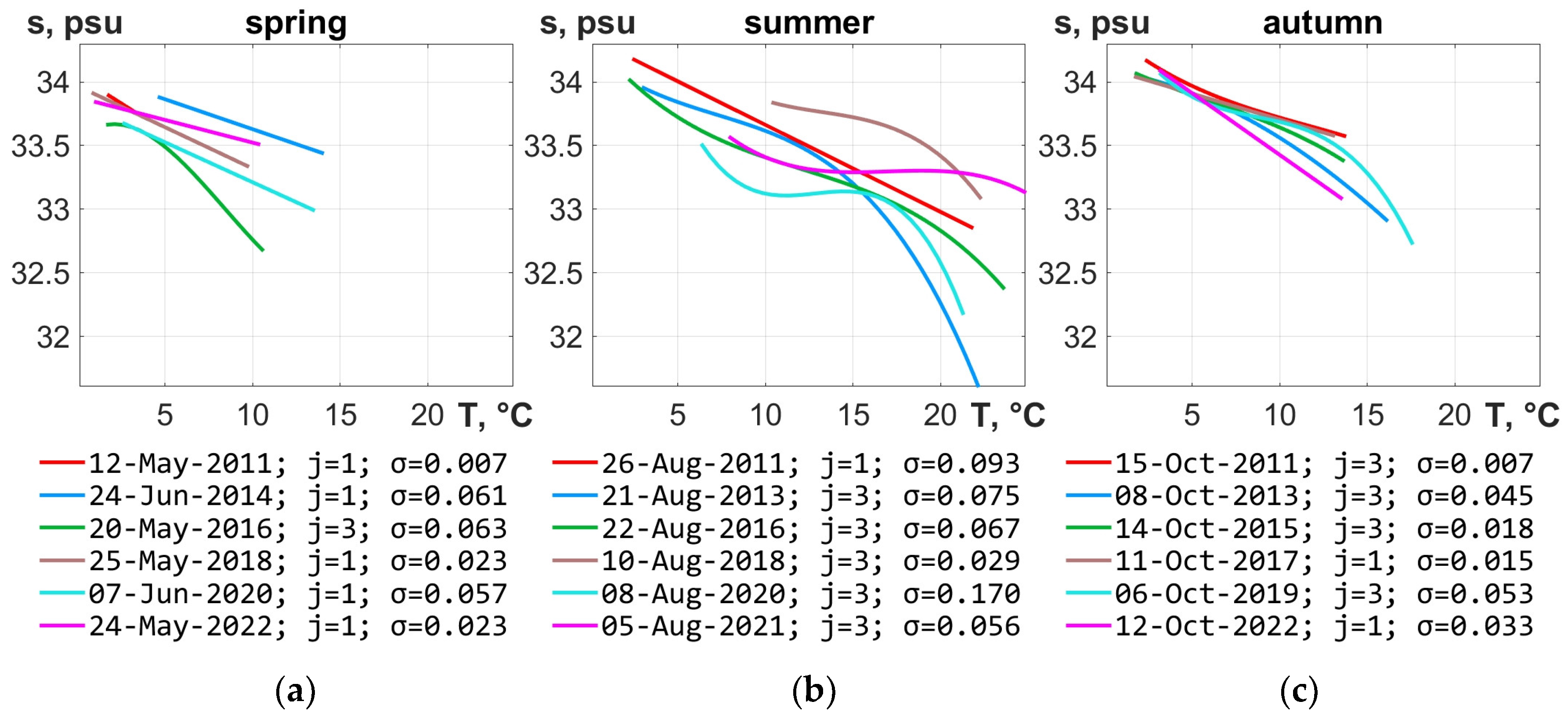
4. Ts Regression Method

To determine the functional dependence of salinity Ts on temperature obtained by a CTD profiler, we propose a model polynomial of the form Y_s = y₀ + y₁T + y₂T² + y₃T³, the order of which is j = {1, 3}. The use of polynomials of a higher order, and splines, did not significantly improve the quality of the regression model. We estimate the accuracy of the degree of conformity of Y_s regression to salinity s, calculated directly from the CTD data, by the value of σ_j(δs)—Root-Mean Square (RMS) of the difference δs = |s − Y_s|. We determine the choice of the order of polynomial j by the empirical condition: when σ₁/σ₃ > 1.2, we use the third-order polynomial, otherwise—the first-order one. When analyzing the data of a series of CTD measurements performed at stations of the same section, to assess the applicability of the Ts regression, we also use σ_av—the value of σ_j averaged over the stations. In some cases, σ_max—the maximum value of σ_j was more applicable for calculations. The value of 2σ is the 95% confidence interval.

Different-scale hydrometeorological processes affecting the water column of the study area of Peter the Great Bay contribute to the spatial inhomogeneity of its thermohaline stratification. For this reason, to resolve the issue of applicability of the model Ts regression within the boundaries of the entire test site, a check of the studied water area for homogeneity of the water composition is required, i.e., it is necessary to investigate how similar the regressions built at different points of the test site are, and whether the regression built based on a set of observation points is universal [2].

One of the climatic features of the coastal regions of the Sea of Japan is tropical cyclones (typhoons), which originate in the area of the Philippine Islands. Every year from June to September, two to five tropical cyclones are recorded in the southern regions of Primorye. Their passage, mainly from the southwest, is always accompanied by heavy precipitation, storm winds, and catastrophic floods on the rivers. For this reason, the second half of summer, especially August, is the most difficult time in terms of maintaining the uniformity of water composition in the offshore areas of Peter the Great Bay.

To monitor the composition of water, on 1 August 2012, within the study area, we performed a series of hydrological sections along the conditional directions S1-S5-Sc-S1 (green circles in Figure 1). The profiling of the water column was carried out with an XRX-620 CTD profiler. In total, 24 profiling was completed within five and a half hours, under moderate wind and smooth seas. The obtained data were processed according to the correction procedure, described in Section 3. When determining the variants of the model Ts regression, due to freshening and uneven heating of the upper layer, we considered the data obtained below the 5 m horizon. The range of temperature T changes at the horizons from 5 to 95 m was 1.0–19.6 °C, salinity s varied within 32.7–34.1 psu; the average salinity s_av was 33.6 psu.

In Figure 7, the red curve Y_s(#10) shows the model cubic polynomial, j = 3, constructed from the profiling data at point #10—the deepest point of the test site; the blue curve Y_s(all)—from the set of all 24 profilings. In the first case, the coefficients of the polynomial y₀ = 34.12; y₁ = −5.9 × 10⁻²; y₂ = 5.1 × 10⁻³; y₃ = −2.7 × 10⁻⁴; in the second—y₀ = 34.17; y₁ = −8.6 × 10⁻²; y₂ = 9.2 × 10⁻³; y₃ = −4.3 × 10⁻⁴. The maximum error in determining salinity from temperature was σ_max(#10) = 0.065 psu and σ_max = 0.052 psu, which allows, for example, the calculation of the speed of sound from T and Y_s with accuracy of 0.16 m/s and 0.13 m/s, respectively (see Table 1). Thus, we have established that in this case the degree of spatial homogeneity of the water composition is acceptable for solving most acoustic and hydrophysical problems, and the polynomial Y_s(all) constructed over the entire set of points will be considered universal within the test site.

We should note that sometimes, mainly immediately after significant HEs, spatial homogeneity of water composition may differ even within the same section. For example, on 13 August 2015, presumably due to a vortex coming onto the Posyet Bay shelf, at three out of nine stations along the S1–S5 route, the Y_s(#) regressions calculated in the temperature range from14 to 24 °C had very different Ts from the rest dependencies with maximum error σ_max = 0.28 psu.

To assess the time intervals of applicability of the obtained Ts regressions, let us analyze the data of hydrological sections made along the S1–S5 route in August 2012. In the study area, during the month, the air temperature varied between 11 and 31 °C, precipitation of varying intensity was observed on 14 days out of 31, and its total volume exceeded 320 mm. In the period from 1 August to 27 August, the wind, as a rule, did not exceed 3–5 m/s, except for 15 August, when it briefly increased to 10–12 m/s. An abrupt increase in wind, with gusts of up to 25 m/s, was observed on 28–29 August 2012, when Typhoon Bolaven came out to the southern coast of Primorye [45]. During this period, our thermostrings were recorded, and CTD profiling was also carried out along the S1–S5 route, so we were able to trace the change in the water composition caused by the HE. According to our observations, the thermohaline structure, which changed under the influence of the typhoon on 28 August, almost returned to its original state by the afternoon of 1 September [21]. To construct regressions, we selected the CTD data obtained at the stations of the S1–S5 route on 1, 27, and 31 August 2012—green, pink, and orange dots in Figure 8, respectively.

As we can see in Figure 8, the model polynomials Y_s(all) almost did not change their coefficients during the month. For each of the days of August—1, 27, and 31, the maximum deviations of the difference δs = |s − Y_s| at the points of Section S1–S5 σ_max were 0.06, 0.06, and 0.11 psu. To assess the applicability of the regressions obtained during the month Ts, we shall perform a cross-calculation of model salinity profiles. The average deviations σ_av established this way for each of the sections are shown in

Table 3. Values of average deviations σ_av for August 2012.

	CTD Data	1 August 2012	27 August 2012	31 August 2012
Polynomial
1 August 2012		0.03	0.09	0.08
27 August 2012		0.05	0.04	0.09
31 August 2012		0.04	0.08	0.06

. As we can see from the table, the Ts regression from 31 August, obtained from the water structure recovering after the HE, provides the lowest accuracy compared to the other two considered polynomials Y_s(all) even for the data of the same day, but it models 1 August quite well. The worst obtained result σ_av = 0.09 psu can provide a calculation of the sound speed with an error not exceeding 0.22 m/s, because ∂c/∂s = 1–1.3 [m/s]/psu (Table 1).

Extreme HEs observed in the area of the test site during one experiment sometimes irreversibly changed the ratio of thermohaline parameters. As a result, the use of the optimal polynomial Y_s, obtained at the beginning of the experiment, after a week already did not make sense for the subsequent modeling of the hydrological picture by the data of thermostrings on the S1–S5 route. For example, Figure 9 shows Ts dependencies obtained in experiments in different seasons when the initial form of regression is not permanent. In the autumn experiment of 2013, under the action of northwesterly wind of 7–12 m/s, the development of local upwelling was recorded on 9–12 October [16]. As a result, the temperature range narrowed from 2–16.5 °C to 2–12 °C, and the optimal Y_s polynomial degenerated from cubic to linear. In August 2017, the narrowing of the temperature range from 4.5–23 °C to 8–22 °C and the change in the degree of the optimal polynomial were affected by the passage of Typhoon Noru on 7–8 August 2017 [21]. During the spring experiment of 2016, restructuring of the thermohaline structure occurred due to a wind surge associated with strong southerly wind on 24 May.

Figure 10 shows regression dependencies built for different seasons of 2011–2022. The values σ_av indicated under the Figures correspond to the RMS of the difference δs = |s − Y_s|, established for each of the presented polynomials. The order of the optimal polynomial j was established according to the accepted criterion σ₁/σ₃ > 1.2. As we can see in Figure 10, in the spring period, the polynomials, except for one, had the first degree; in summer, on the contrary, the model dependencies were cubic in five out of six cases. In autumn, linear dependencies were observed in two cases out of the six presented.

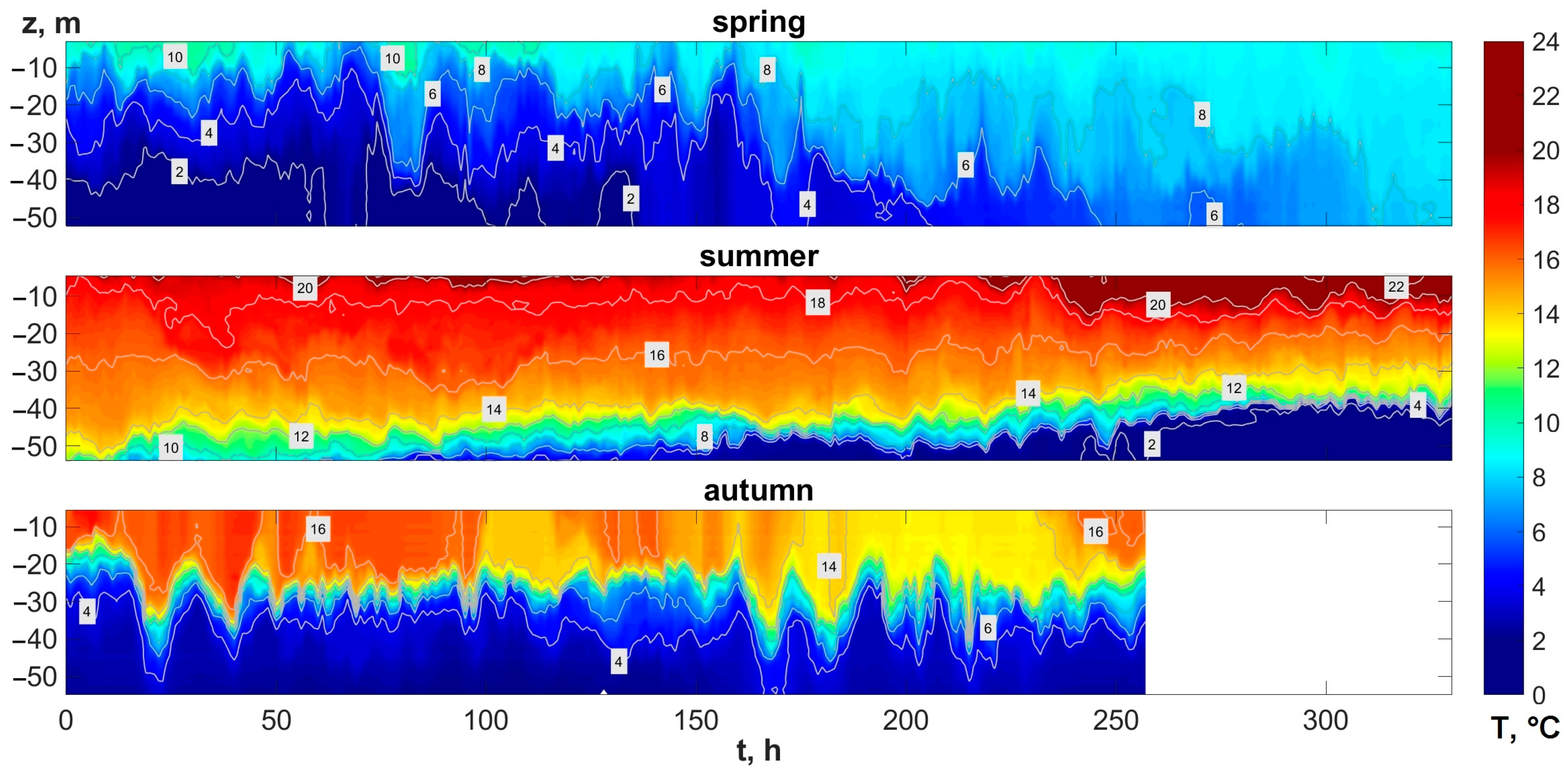
5. Examples of Using Temperature Sensors for Monitoring Hydrophysical Processes

Let us now consider two examples of using thermostrings data and the Ts regression method to analyze various hydrophysical processes in 2022. The change of buoyancy frequency distribution with depth over many hours of observation is discussed in Section 5.1. Furthermore, in Section 5.2, we estimate sound speed fluctuations caused by internal waves and discuss the relationship between sound speed variations and isopycnal shifts.

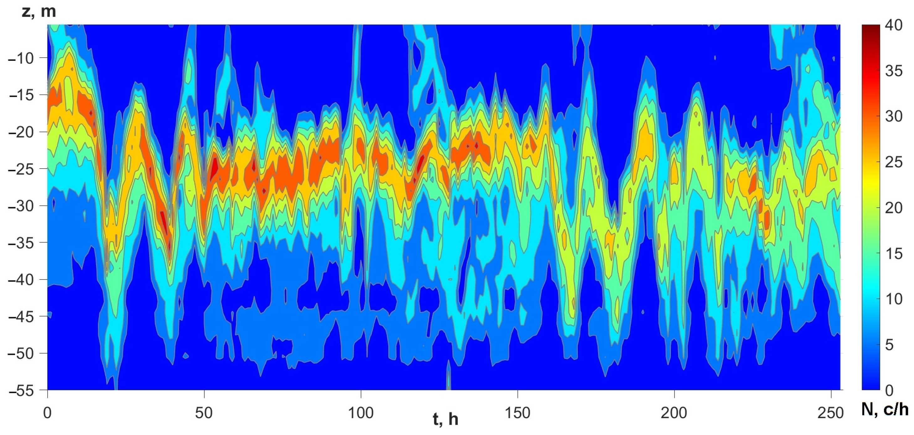
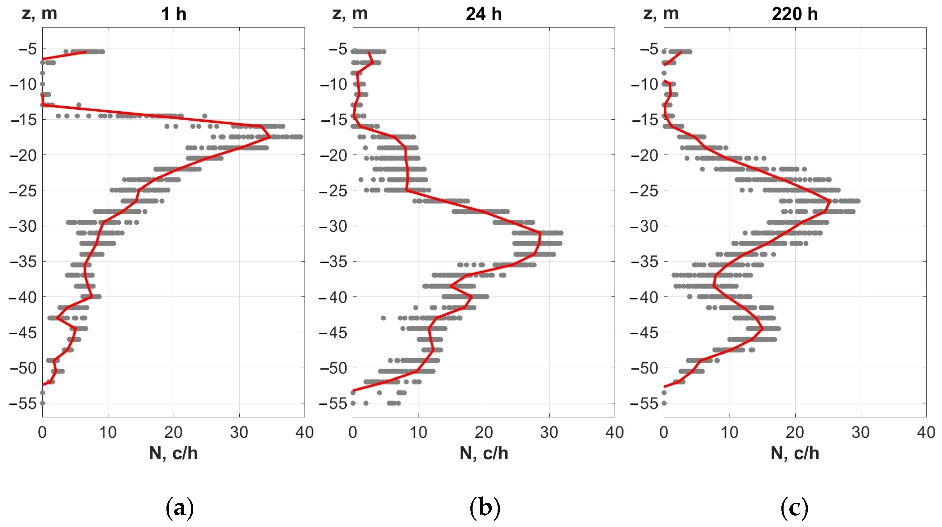
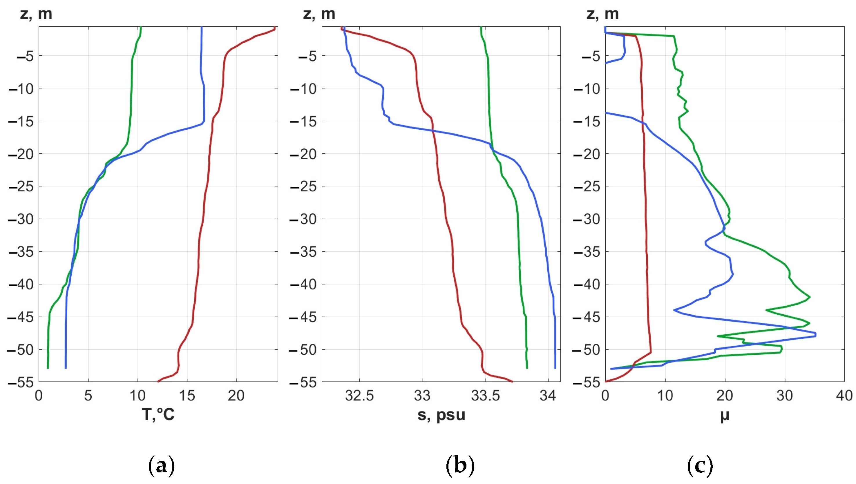
5.1. Space–Time Distributions of the Buoyancy Frequency

Prediction of wave modes in the seas requires detailed knowledge of the vertical structure of the hydrophysical characteristics of water over long periods of observation. According to theoretical concepts, the parameters of nonlinearity and coefficient of nonlinear internal waves’ dispersion are determined by the eigenfunctions of the Sturm-Liouville problem. The determining factor of these eigenfunctions form is the buoyancy frequency N(z) as a function of the site depth [46,47]. In turn, the buoyancy frequency varies not only in space but also in time. Such variations in the buoyancy frequency are one of the reasons for fluctuations of packets of nonlinear internal waves observed in long-term experiments [48]. To estimate the coefficients of evolutionary equations and predict the parameters of nonlinear wave motions, it is customary to use some average values, which can sometimes be found in international databases. Using field measurements of hydrological characteristics allows the estimation of the limits of applicability of averaged wave models when only averaged profiles of buoyancy frequency are used [49].

Figure 11 shows the distribution of the buoyancy frequency averaged over 1 h at a point with a depth of 56 m in autumn 2022. The buoyancy frequency was calculated from the S4 thermostring data using linear Ts regression. To estimate the regression coefficients, we used CTD data obtained at this point on 3, 8, and 12 October. The temperature, measured by a thermostring in the layer of 5.5–55 m at 34 horizons with a step of 1 min from 3 October to 14 October 2022, is shown in Figure 3. As we can see in Figure 3 and Figure 11, the water layer under study had temperatures from 2 to 18 °C and was characterized by thermocline thickness of 12–20 m with a gradient of more than 2 °C/m. At the same time, during the tidal cycle of 12.4 h, it sometimes performed vertical oscillations of up to 20 m.

Variations in time N(z) are significantly determined by fluctuations in the depth of the thermocline position, which we can see if we compare Figure 3 and Figure 11. The values of N(z) in the first half of the experiment reach 38 c/h (cycles per hour), and in the second part, they become less than 30 c/h. Figure 12 shows instantaneous values of buoyancy frequency in three 1-h intervals 0–1 h, 23–24 h, and 219–220 h, and also the corresponding averaged profiles.

As we know, the average value of the buoyancy frequency is usually calculated from the average density over a selected time interval [50]. Since the density changes little, and the differentiation operation is linear, such an operation corresponds to the usual time averaging of the instantaneous value N(z). However, this approach applies to the deep ocean, where tidal motions change the position of the thermocline only slightly. In the case of a coastal zone, tidal waves significantly change the position of the thermocline in the water layer, as a result, when averaging over periods of more than a semidiurnal tide, typical functional dependence N(z) is distorted. Figure 13 shows the N(z) curves averaged over time intervals Δt = {1 h, 6 h, 12 h}. The values of N(z) averaged over the time interval Δt =12 h (Figure 13c) already have a structure that is not typical for this region.

The same Figure 13 shows the N(z) curves obtained by another method, marked in red: we averaged the isopycnal positions over time, from which we then formed the vertical profile of the “average” density and calculated the N(z) values. We can see that these “average” N(z) at small averaging intervals of 1 h (Figure 13a) and 6 h (Figure 13b) are close to the usual average N(z). For the averaging interval of 12 h (Figure 13c), they retain the structure of the instantaneous buoyancy frequency, and the position of the peak of this curve corresponds to the average value of the peaks of all instantaneous N(z). Despite the physical clarity of this approach, it still requires further mathematical justification.

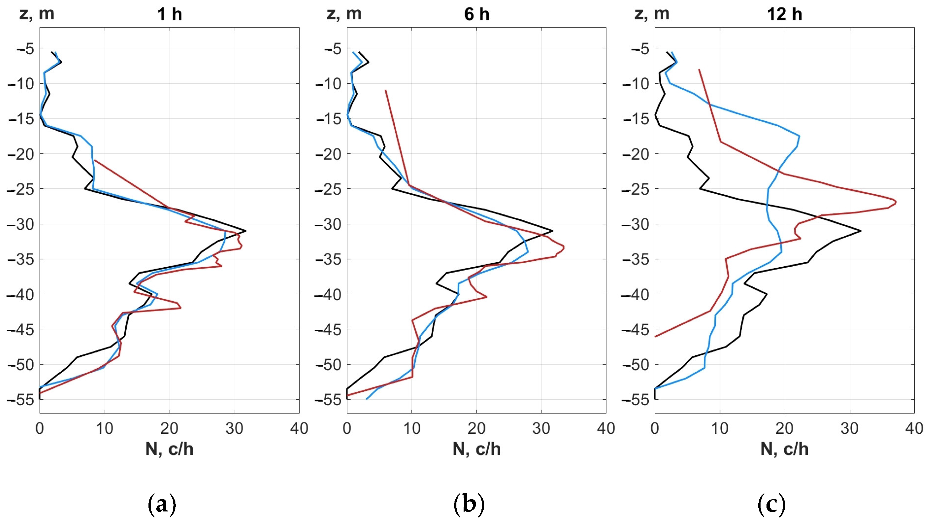
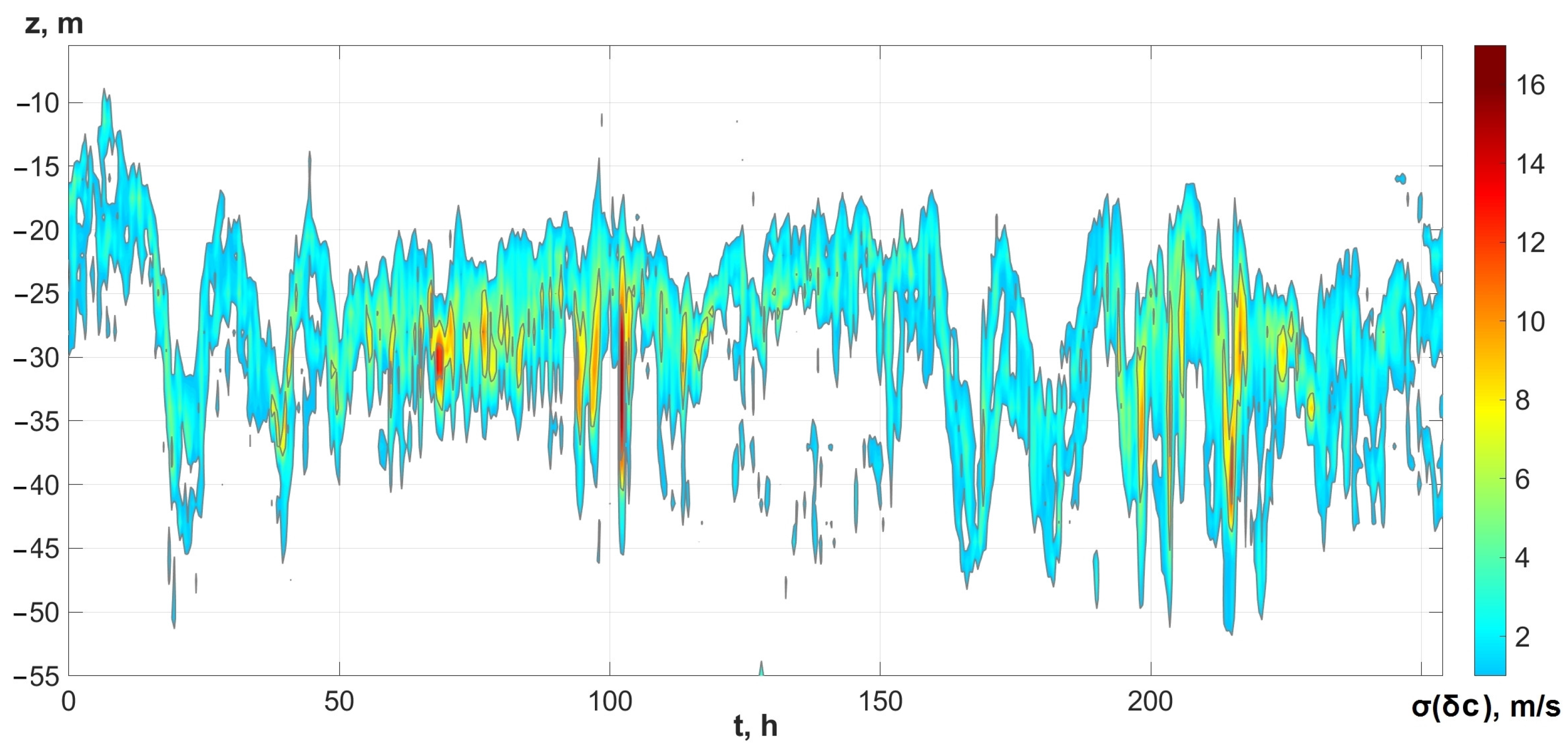
5.2. Fluctuations of Sound Speed in the Field of Internal Waves

The main cause of sound speed fluctuations both in the deep ocean and in its shelf zone are internal waves [35,51]. Background (linear) IWs are always present on the shelf, the same as in the deep ocean. Unlike soliton-like nonlinear waves, they represent a field that can be considered random in a certain sense. The main specificity of background waves on the shelf is that not free waves, but residual perturbations of small amplitudes of trains of nonlinear waves, can make a significant contribution to the background field. Such “tails” are both quite long in time and extended in space. If we consider the speed of sound, perturbed by the IW field, then formally it can be written as c(t,x,y,z) = <c(t,x,y,z)> + δc(t,x,y,z). Here the angle brackets mean the operation of averaging, and the value δc describes the random part, which is obtained by subtracting its middle part from the observed sound speed field. Let us note that such a representation requires a preliminary choice of characteristic space and time scales of the sound speed field, over which averaging is performed. Thus, fluctuations c(t,x,y,z) are determined by the maximum scales for inhomogeneities, which we decided to classify as fluctuations. Naturally, such a choice is ambiguous, it is conditional and is determined by the physical meaning of a specific task; for example, the problem of IW sound scattering over a certain time interval [8].

According to studies, in the presented region, IW fluctuations at frequencies higher than 2–2.5 c/h (periods from 30 to 24 min) are “stochasticized” and are well described by Gaussian distribution [52]. Therefore, further, for the sake of definiteness, we assume that <c(t,z)> is the average speed of sound over the time interval of 30 min, and we consider δc(t,z) = c(t,z) − <c(t,z)> its fluctuations over the same time interval.

Figure 14 shows the RMS value of fluctuations in the sound speed σ over the entire depth of the water layer throughout the entire time of the experiment, where σ²(δc) = [<(δc)²> − <δc>²]. As in the case of determining the buoyancy frequency, the values c(t,z) were calculated from the data of thermostring S4 using the regression. Comparison of c(t,z) with distributions T(t,z) and N(t,z) (Figure 3 and Figure 11) shows that main fluctuations of sound speed with amplitudes σ(δc) ≈ 1–2 m/s are observed in the thermocline and values σ(δc) up to 4–10 m/s are observed more seldom. Outside the thermocline, the values of σ(δc) are at least an order of magnitude smaller than those indicated above.

For small fluctuations in sound speed, it is customary in hydroacoustics to use the following relationship between δc(t,z) and the value of vertical displacement of fluid particles ζ [51,53]:

$$\delta c={\left(\frac{\partial c}{\partial z}\right)}_{pot}\zeta , \delta c=c \left(\frac{\mu }{g}\right) N^2 \zeta .$$

(12)

Here the potential gradient of sound speed is indicated, μ ≈ 24.5 is a dimensionless constant, and g = 9.8 m/s² is the gravitational acceleration. Formula (12) provide a simple connection between the statistics ζ(t,z) and δc(t,z). The second part of Formula (12) has gained particular popularity. It is used by many researchers to model fluctuations δc(t,z) both in deep oceans and in shallow seas [35,51].

For the first time, the second part of Formula (12) was obtained in [53], where the authors studied the effect of linear internal waves on sound fluctuations in deep oceans. The parameter μ, included in (12), is determined by a set of thermodynamic parameters that combine variations in sound speed, density, temperature, and salinity. Moreover, the variability of the μ parameter itself depends on the ratio of salinity and potential temperature gradients (the “Turner number”), which, in the case of deep oceans, change insignificantly; therefore, all parameters in [53] were chosen for the depth of 1 km. As a result, the value of μ ≈ 24.5 was obtained; however, wide ranges of temperature and salinity variability are observed in the shelf zone (Figure 3). Accordingly, variations in the parameter μ are inevitable due to multiple changes (several times) in the derivatives of thermodynamic parameters (see Table 1).

From the CTD profiling data for different seasons, the values of μ were calculated both by the formulas of [53], using a set of thermodynamic parameters, and from a simple equation following from Formula (12):

$$\mu =\frac{g}{c} {\left(\frac{\partial c}{\partial z}\right)}_{pot} N^{-2}.$$

(13)

Figure 15 shows the distributions of temperature (Figure 15a), salinity (Figure 15b), and the μ(z) function (Figure 15c) in three seasons of 2022. Here, μ was calculated by the method of [53], and for control, calculations were also carried out using formula (13). Determining the values of thermodynamic parameters, we used CTD data from RBRconcerto, measured at point S4. Good coincidence between different calculations ensured the reliability of the result.

As you can see in Figure 15c, μ is a function of the z-coordinate and depends on time. During the measurement periods of 2022, the value of μ, depending on the depth, changed in the range from 0 to 36. We also performed similar calculations based on CTD data obtained in different seasons of 2016 and 2019, according to which this function varied in the range from 1 to 40 and had a noticeable seasonal variability.

Thus, for the shelf zone in the model descriptions of IWs, it is necessary to take into account that in Formula (12) μ is not a constant, but a function that changes significantly not only with depth but also with time.

6. Conclusions

High-precision measurements of salinity and temperature in the seawater column are carried out, as a rule, using a CTD profiler from a board of a specialized vessel. During long-term observations in a chosen point or area, the variability of weather conditions imposes an additional limitation on the technical capabilities of the experimenters. In this regard, the optimal solution is the long-term setup of anchored thermostrings.

However, for several hydroacoustic and hydrophysical problems on the shelf, in addition to thermostrings, it is necessary to know the salinity with certain optimal accuracy. For example, to study background fluctuations in the sound speed, when amplitudes of these fluctuations are 1–2 m/s, it is required to measure salinity with an accuracy of 0.1–0.2 psu, because əc/əs ≈ 1 [m/s]/psu (Figure 14). Increased requirements for the accuracy of determining the density of water may also arise for calculating the equations of multilayer shallow water [54]. The range of salinity variation in the study area of Peter the Great Bay (the Sea of Japan) is about 3 psu, which is why using some average salinity for solving the set tasks is unacceptable.

From data of many years from CTD profiling at the hydrophysical test site in the shelf zone of Peter the Great Bay, the authors obtained regression formulas for calculating salinity from temperature with the required accuracy. It was established that the stability of regression dependence is determined by the degree of spatial homogeneity of the water composition. Thermohaline structure in the area of the test site may change upon the onset of one of the hydrometeorological events (HEs): entry of a mesoscale vortex into the water area, upwelling, passing of a typhoon, etc. On average, on time scales of the order of one week, the regression dependence is permanent. In the time intervals between HEs, the stability of regression dependence over the test site space was established, when functional dependence Ts was permanent in the water area with an accuracy of 0.2 psu.

During 12 years of monitoring, we observe a certain recurrence of the functional relationship between temperature and salinity by season. In different years, as a rule, the degree of the regression polynomial is preserved, but in some years, in spring and autumn, its coefficients also may change slightly (Figure 10). Thus, in spring, the regression is mainly polynomials of the 1st order; and rare polynomials of the 3rd order are close to a linear function. In autumn, on the contrary, regression is mainly the 3rd-order polynomials located in a close group in the figure. The most complex regression pattern in summer is the 3rd-order polynomials with considerably varying coefficients. This situation arises because in summer this area is subject to a stronger and more frequent influence of HEs, which change the composition of water more intensively than in other seasons.

Based on the selected data, it was established that to describe the functional dependence of T and s, it is sufficient to use polynomials of up to the 3rd order. The use of polynomials of a higher order, as well as splines, did not significantly improve the quality of the regression model.

An important step in constructing Ts regressions is the preliminary primary processing of CTD profiling data. The purpose of such processing is to minimize dynamic errors of CTD data, which are especially great in the coastal zone due to high-temperature gradients. Dynamic errors in the measured temperature and salinity in the selected area can reach values of 0.2 °C and 0.5 psu or more, which is unacceptable for using such regressions to solve the problems mentioned above. Solutions for processing raw CTD data offered by profilers’ manufacturers did not always provide the required accuracy in our experiments. Therefore, based on many years of experience in the coastal zone, the authors have developed and proposed original methods for the dynamic correction of CTD data.

It was demonstrated in the work that in the coastal zone of the sea, the combined use of data from thermostrings and CTD profilers (Ts regressions) allows the efficient investigation of the space–time variability of the buoyancy frequency and sound speed fluctuations on the average for one week in the absence of HEs. Accordingly, additional CTD measurements should be planned regarding weather forecasts, meteorological observations, and satellite data. In the future, when organizing such test site work, it will be possible to avoid the necessity of monitoring HEs using setups of scanning systems of the “Aqualog profiler” type, which allow the measurement of salinity for a long time at all horizons of the water column [55].

References

1. Thacker, W.C.; Lee, S.K.; Halliwell, J. Assimilating 20 Years of Atlantic XBT Data Into HYCOM: A First Look. Ocean Model. 2004, 7, 183–210. [Google Scholar] [CrossRef]
2. Korotenko, K.A. A regression method for estimating salinity in the Ocean. Oceanology 2007, 47, 464–475. [Google Scholar] [CrossRef]
3. Thacker, W.C. Estimating salinity to complement observed temperature: 1. Gulf of Mexico. J. Mar. Syst. 2007, 65, 224–248. [Google Scholar] [CrossRef]
4. Thacker, W.C.; Sindlinger, L. Estimating salinity to complement observed temperature: 2. Northwestern Atlanic. J. Mar. Syst. 2007, 65, 249–267. [Google Scholar] [CrossRef]
5. Shtokman, V.B. Principles of the theory of T–s curves as a method for study of the mixing and transformation of water masses. Problemy Artiki 1943, 1, 32–71. (In Russian) [Google Scholar]
6. Mamayev, O.I. Temperature—Salinity Analysis of Word Ocean Water; Elsevier: Amsterdam, NY, USA, 1975. [Google Scholar]
7. Stommel, H. Note on the Use of the T,S-Correlation for Dynamic Height Anomaly Calculations. J. Marine Res. 1947, 1, 85–92. [Google Scholar]
8. Flierl, G.R. Correcting Expendable Bathythermograph (XBT) Data for Salinity Effects to Compute Dynamic Heights in Gulf Stream Rings. Deep-Sea Res. 1978, 25, 129–134. [Google Scholar] [CrossRef]
9. Vossepoel, F.C.; Reynolds, R.W.; Miller, I. Use of Sea Level Observations to Estimate Salinity Variability in Tropical Pacific. J. Atmos. Ocean Technol. 1999, 16, 1401–1415. [Google Scholar] [CrossRef]
10. Dorfschafer, G.S.; Tanajura, C.A.S.; Costa, F.B.; Santana, R.C. A new approach for estimating salinity in the Southwest Atlantic and its application in a data assimilation evaluation experiment. JGR Oceans. 2020, 125, e2020JC016428. [Google Scholar] [CrossRef]
11. Hansen, D.V.; Thacker, W.C. Estimation of Salinity Profiles in the Upper Ocean. J. Geophys. Res. 1999, 104, 7921–7933. [Google Scholar] [CrossRef]
12. Pivovarov, A.A.; Yaroshchuk, I.O.; Dolgikh, G.I.; Shvyrev, A.N.; Samchenko, A.N. An Autonomous Acoustic Logger and Its Application as Part of a Hydrophysical Complex. Instrum. Exp. Technol. 2021, 64, 468–473. [Google Scholar] [CrossRef]
13. Pivovarov, A.A.; Yaroshchuk, I.O.; Shvyrev, A.N.; Samchenko, A.N. An autonomous low-frequency broadband hydroacoustic emitting station with electromagnetic transducer. Instrum. Exp. Technol. 2020, 63, 880–884. [Google Scholar] [CrossRef]
14. Yaroshchuk, I.O.; Leont’ev, A.P.; Kosheleva, A.V.; Pivovarov, A.A.; Samchenko, A.N.; Stepanov, D.V.; Shvyryov, A.N. On intense internal waves in the coastal zone of the Peter the Great Bay (the Sea of Japan). Russian Meteorol. Hydrol. 2016, 41, 629–634. [Google Scholar] [CrossRef]
15. Kukarin, V.F.; Liapidevskii, V.Y.; Khrapchenkov, F.F.; Yaroshchuk, I.O. Nonlinear internal waves in the shelf zone of the sea. Fluid Dyn. 2019, 54, 329–338. [Google Scholar] [CrossRef]
16. Kosheleva, A.V.; Yaroshchuk, I.O.; Khrapchenkov, F.F.; Pivovarov, A.A.; Samchenko, A.N.; Shvyrev, A.N.; Korotchenko, R.A. Upwelling on the Narrow Shelf of the Sea of Japan in 2011. Fundam. I Prikl. Gidrofiz. 2021, 14, 31–42. [Google Scholar] [CrossRef]
17. Gulin, O.E.; Yaroshchuk, I.O. Dependence of the mean intensity of a low-frequency acoustic field on the bottom parameters of a shallow sea with random volumetric water-layer inhomogeneities. Acoust. Phys. 2018, 64, 186–189. [Google Scholar] [CrossRef]
18. Leontyev, A.P.; Yaroshchuk, I.; Smirnov, S.; Kosheleva, A.; Pivovarov, A.A.; Samchenko, A.; Shvyrev, A. A spatially distributed measuring complex for monitoring hydrophysical processes on the ocean shelf. Instrum. Exp. Technol. 2017, 60, 130–136. [Google Scholar] [CrossRef]
19. Korotchenko, R.A.; Samchenko, A.N.; Yaroshchuk, I.O. The spationtemporal analysis of the bottom geomorphology in Peter the Great Bay of the Sea of Japan. Oceanology 2014, 54, 497–504. [Google Scholar] [CrossRef]
20. Navrotsky, V.V.; Izergin, V.L.; Pavlova, E.P. Generation of internal waves near the shelf boundary. Dokl. Earth Sci. 2003, 388, 84–88. Available online: https://www.researchgate.net/publication/297414462 (accessed on 1 April 2023).
21. Samchenko, A.; Dolgikh, G.; Yaroshchuk, I.; Kosheleva, A.; Pivovarov, A.; Novotryasov, V. Extreme Hydrometeorological Conditions of Sediment Waves’ Formation and Migration in Peter the Great Bay (The Sea of Japan). Water 2023, 15, 393. [Google Scholar] [CrossRef]
22. Trusenkova, O.O.; Lobanov, V.B.; Lazaryuk, A.Y. Currents in the Southwestern Peter the Great Bay, the Sea of Japan, from the Stationary Wavescan Buoy Data in 2016. Oceanology 2022, 62, 310–323. [Google Scholar] [CrossRef]
23. Dubina, V.A.; Lobanov, V.B.; Mitnik, L.M. Features of the surface circulation in the Northwestern Japan Sea from ERS synthetic aperture radar data. In Oceanography of the JAPAN Sea. Proc. CREAMS’2000 Int. Symp.; Danchenkov, M.A., Ed.; Dalnauka: Vladivostok, Russia, 2001; pp. 166–173. [Google Scholar]
24. Operator’s Manual. Model SBE 19plus, SEACAT Profiler. Sea-Bird Electronics, Inc. USA. Available online: http://www.seabird.com (accessed on 1 April 2023).
25. Operator’s Manual. Model XR-620 and XRX-620. Richard Brancker Research Ltd., Canada. Available online: www.rbr-global.com (accessed on 1 April 2023).
26. IOC; SCOR; IAPSO. The International Thermodynamic Equation of Seawater—2010: Calculation and Use of Thermodynamic Properties; Intergovernmental Oceanographic Commission, Manuals and Guides; UNESCO: Paris, France, 2010; No. 56. [Google Scholar]
27. Arkhipkin, V.S.; Lazaryuk, A.Y.; Levashov, D.E.; Ramazin, A.N. Oceanology. Instrumental Methods for Measuring the Main Parameters of Sea Water; MAKS Press: Moskva, Russia, 2009; 335p. (In Russian) [Google Scholar]
28. Lazaryuk, A.Y. Response functions of the temperature and conductivity sensors of CTD profilers. Oceanology 2008, 48, 872–875. [Google Scholar] [CrossRef]
29. Lazaryuk, A.; Ponomarev, V.; Salyuk, A. Mismatching of raw MARK-IIIC CTD data. Pac. Oceanogr. 2008, 4, 59–62. [Google Scholar]
30. Trump, C.L. Effects of ship’s roll on the quality of precision CTD data. Deep-Sea Res. 1983, 30, 1173–1183. [Google Scholar] [CrossRef]
31. Emery, W.J.; Thomson, R.E. Data Analysis Methods in Physical Oceanography, 3rd ed.; Elsevier: Amsterdam, The Netherlands, 2014; 716p. [Google Scholar] [CrossRef]
32. The Practical Salinity Scale 1978 and the International Equation of State of Seawater 1980. In UNESCO Technical Papers in Marine Science; UNESCO: Paris, France, 1981; No. 36; pp. 13–21. Available online: https://www.jodc.go.jp/jodcweb/info/ioc_doc/html/UNESCO_Tech.htm (accessed on 1 April 2023).
33. UNESCO Technical Papers in Marine Science. The Acquisition, Calibration, and Analysis of CTD Data; UNESCO: Paris, France, 1988; No. 54; Available online: https://www.jodc.go.jp/jodcweb/info/ioc_doc/html/UNESCO_Tech.htm (accessed on 1 April 2023).
34. Lueck, R.G.; Picklo, J.J. Thermal inertia of conductivity cells: Observations with a Sea-Bird Cell. J. Atmos. Oceanic Technol. 1990, 7, 756–768. [Google Scholar] [CrossRef]
35. Katsnelson, B.; Petnikov, V.; Lynch, J. Fundamentals of Shallow Water Acoustics; Springer: New York, NY, USA, 2012; 540p. [Google Scholar] [CrossRef] [Green Version]
36. Bennett, A.S.; Huaide, T. CTD time-constant correction. Deep-Sea Res. 1986, 33, 1425–1438. [Google Scholar] [CrossRef]
37. Operator’s Manual. SBE Data Processing 7.23.2. Available online: http://www.seabird.com (accessed on 1 April 2023).
38. Halverson, M.; Jackson, J.; Richards, C.; Melling, H.; Brunsting, R.; Dempsey, M.; Gatien, G.; Hamilton, A.; Jacob, W.; Zimmerman, S.; et al. Guidelines for processing RBR CTD profiles. Can. Technol. Rep. Hydrogr. Ocean Sci. 2017, 314, iv + 38 p. [Google Scholar]
39. Bendat, J.S.; Piersol, A.G. Random Data: Analysis and Measurement Procedures, 4th ed.; Wiley: Hoboken, NJ, USA, 2010; 640p. [Google Scholar]
40. Giles, A.B.; McDougall, T.J. Two methods for the reduction of salinity spiking of CTD’s. Deep-Sea Res. 1986, 33, 1253–1274. [Google Scholar] [CrossRef]
41. Millard, R.; Toole, J.; Swartz, M. A fast responding temperature measurement system for CTD application. IEEE J. Ocean. Eng. 1980, 7, 413–427. [Google Scholar] [CrossRef]
42. Smirnov, G.V.; Eremeev, V.N.; Ageev, M.D.; Korotaev, G.K.; Yastrebov, V.S.; Motyzhev, S.V. Oceanology: Methods of Oceanographic Study; Nayka: Moscow, Russia, 2005. (In Russian) [Google Scholar]
43. Post-Processing RBR Data with RSKtools; RSKtools v3.5.0. RBR Ltd.: Ottawa ON, Canada, 2020. Available online: https://rbr-global.com/wp-content/uploads/2020/06/PostProcessing.pdf (accessed on 1 April 2023).
44. RSKtools 3.5.3. Available online: http://www.rbr-global.com/support/matlab-tools (accessed on 1 April 2023).
45. Digital Typhoon. Available online: http://agora.ex.nii.ac.jp/digital-typhoon (accessed on 25 March 2023).
46. Talipova, T.G.; Pelinovsky, E.N.; Kurkin, A.A.; Kurkina, O.E. Modeling the Dynamics of Intense Internal Waves on the Shelf. Izv. Atmos. Ocean. Phys. 2014, 50, 630–637. [Google Scholar] [CrossRef]
47. Badiey, M.; Wan, L.; Lynch, J.F. Statistics of nonlinear internal waves during the Shallow Water 2006 Experiment. J. Atmos. Ocean. Technol. 2016, 33, 839–846. [Google Scholar] [CrossRef]
48. Colosi, J.A.; Kumar, N.; Suanda, S.H.; Freismuth, T.M.; MacMahan, J.H. Statistics of internal tide bores and internal solitary waves observed on the continental shelf of Point Sal, California. J. Phys. Oceanogr. 2018, 48, 123–143. [Google Scholar] [CrossRef] [Green Version]
49. Ivanov, V.A.; Pelinovsky, E.N.; Talipova, T.G.; Troitskaya, Y.I. Statistical estimations of the parameters of non-linear long internal waves off the South Crimea in the Black Sea. Phys. Oceanogr. 1995, 6, 253–261. [Google Scholar] [CrossRef]
50. Dijkstra, H.A. Dynamical Oceanography; Springer: Berlin/Heidelberg, Germany, 2008. [Google Scholar] [CrossRef]
51. Flatte, S.; Dashen, R.; Munk, W.; Watson, K.; Zachariasen, F. Sound Transmission through a Fluctuating Ocean; Cambridge U.P.: Cambridge, UK, 1979; 320p. [Google Scholar]
52. Kosheleva, A.; Yaroshchuk, I.; Shvyrev, A.; Samchenko, A.; Pivovarov, A.; Gulin, O.; Korotchenko, R.; Yaroshchuk, E. Specific features of high-frequency component of background internal gravity waves on the shelf of the Sea of Japan. FEFU Sch. Eng. Bull. 2020, 43, 96–105. (In Russian) [Google Scholar] [CrossRef]
53. Munk, W.H.; Zachariasen, F. Sound propagation through a fluctuating stratified ocean: Theory and observation. J. Acoust. Soc. Am. 1976, 59, 818–838. [Google Scholar] [CrossRef]
54. Liapidevskii, V.Y.; Khrapchenkov, F.F.; Chesnokov, A.A.; Yaroshchuk, I.O. Modeling of unsteady geophysical processes on the shelf of the Sea of Japan. Fluid Dyn. 2022, 57, 55–65. [Google Scholar] [CrossRef]
55. Trusenkova, O.O.; Ostrovskii, A.G.; Lazaryuk, A.Y.; Lobanov, V.B. Evolution of the Thermohaline Stratification in the Northwestern Sea of Japan: Mesoscale Variability and Intra-annual Fluctuations. Oceanology 2021, 61, 319–328. [Google Scholar] [CrossRef]
Figure 1. Scheme of measuring equipment setup and points of CTD profiling. Triangles are thermostrings; dark—regular locations; light—irregular locations. Green circles are places of CTD profiling.
Jmse 11 01204 g001
Figure 2. Ranges of (a) temperature and (b) salinity changes at depth levels from the surface to 54 m for all CTD profiling at the hydrophysical test site for the period of 2011–2022. Green lines are spring; red lines are summer; blue lines are autumn.
Jmse 11 01204 g002
Figure 3. Temperature distribution in depth according to the S4 thermostring in different seasons of 2022. The numbers indicate the temperature values of the selected isotherms.
Jmse 11 01204 g003
Figure 4. Results of CTD SBE 19plus profiling in August 2014 at point S1. The black curves are temperature T1(z) and salinity s1(z) = s(E1, T1, p1) as produced by the profiler software; the blue curve s2(z) is the result of processing by the SBE-Data Processing program; the red curve s3(z) is the salinity obtained as a result of the scheme (8–10); green curve—ΔT = |T1T2|; purple—ΔT = |T1T3|.
Jmse 11 01204 g004
Figure 5. Results of CTD RBR XR-620 profiling at the beginning of September 2011 at point S2. The black curves are temperature T1(z) and salinity s1(z) = s(E1, T1, p1) as produced by the profiler software; red curve s3(z)—the result of processing by method (8–10); purple curve—ΔT = |T1T3|.
Jmse 11 01204 g005
Figure 6. CTD XR-620 data in mid-August 2011 in conditions of pitching and rolling at point S2. The black curves are temperature T1(z) and salinity s1(z) = s(E1,T1,p1) as produced by the profiler software; the red curve s3(z) is the result of processing by method (8)–(10); the blue curve is the speed of the profiler movement in conditions of pitching and rolling of the vessel.
Jmse 11 01204 g006
Figure 7. T and s values from CTD measurements on 1 August 2012. Green dots are processed data at point #10; gray dots are processed data at other points of the test site; the red line is Ys at point #10; the blue line is for the total set of all points.
Jmse 11 01204 g007
Figure 8. The values of T and s from CTD measurements on the S1–S5 route in August 2012 are dots, and the optimal polynomials Ys(all) obtained from them are solid lines.
Jmse 11 01204 g008
Figure 9. Optimal polynomials Ys(all) established from October 2013 data are blue lines; May 2016 are green lines; and August 2017 are red lines. Solid lines are Ts regressions at the beginning of the observation period; dotted lines are those at the end of that period.
Jmse 11 01204 g009
Figure 10. Optimal polynomials Ys for: (a) spring, (b) summer, and (c) autumn seasons of 2011–2022, their order—j and RMS—σ.
Jmse 11 01204 g010
Figure 11. Depth distribution of buoyancy frequency N(z) at point S4 in the period of 3–14 October 2022.
Jmse 11 01204 g011
Figure 12. Depth distribution of the buoyancy frequency N(z), averaged over one hour at different times from the beginning of the experiment: (a) 0–1 h; (b) 23–24 h; (c) 219–220 h. The dots show the instantaneous values of buoyancy frequency during the averaging time Δt = 1 h.
Jmse 11 01204 g012
Figure 13. Average values of buoyancy frequency N(z). Black curves—instantaneous values of N(z); blue curves—N(z) averaged over time intervals Δt: (a) 1 h; (b) 6 h; (c) 12 h. Red curves are N(z), calculated from the density obtained by averaging the isopycnal positions over the same time intervals.
Jmse 11 01204 g013
Figure 14. RMS values of fluctuations of sound speed σ(δc) at the point S4 in the period 3–14 October 2022.
Jmse 11 01204 g014
Figure 15. Instantaneous distributions of (a) temperature, (b) salinity, and (c) parameter μ, depending on the depth, at the point S4 in different seasons of 2022. Green curves—22 May; red—31 July; blue—3 October.
Jmse 11 01204 g015