Article

Collision Avoidance Strategy for Unmanned Surface Vessel Considering Actuator Faults Using Kinodynamic Rapidly Exploring Random Tree-Smart and Radial Basis Function Neural Network-Based Model Predictive Control

School of Marine Science and Technology, Northwestern Polytechnical University, Xi’an 710072, China
*
Author to whom correspondence should be addressed.
J. Mar. Sci. Eng. 2023, 11(6), 1107; https://doi.org/10.3390/jmse11061107
Submission received: 28 April 2023 / Revised: 18 May 2023 / Accepted: 21 May 2023 / Published: 23 May 2023
(This article belongs to the Special Issue Autonomous Marine Vehicle Operations)

Abstract

:
Path planning and tracking are essential technologies for unmanned surface vessels (USVs). The kinodynamic constraints and actuator faults, however, bring difficulties in finding feasible paths and control efforts. This paper proposes a collision avoidance strategy for USV by developing the kinodynamic rapidly exploring random tree-smart (kinodynamic RRT*-smart) algorithm and the fault-tolerant control method. By utilizing the triangular inequality and the intelligent biased sampling strategy, the kinodynamic RRT*-smart shows its advantages in terms of path length, cost and running time. With consideration of kinodynamic constraints, a feasible and collision-free trajectory can be provided. Then, a radial basis function neural network-based model predictive control (RBF-MPC) method was designed that compensates for the model’s uncertainties by developing the radial basis function neural network (RBF-NN) approximator and by constructing a feedback-state training dataset in real time. Furthermore, two types of fault situation were analyzed considering the thruster failure. We established the faults’ mathematical models and investigated the fault-tolerant strategies for different fault types. The simulation studies were conducted to validate the effectiveness of the proposed strategy. The results show that the proposed planning and control methods can avoid obstacles in faulty conditions.

1. Introduction

Unmanned surface vessels (USVs), as an intelligent water work platform, have been widely used in oceanic exploration, personnel search and rescue, water surface cleaning and other aspects [1,2,3,4,5]. Compared with man-operated ships, USVs are not only more economical and safe but are also more suitable for harsh environments, which attracts enormous attention from both the academic and industrial fields. Planning a path that aligns harmoniously with its own motion properties is an indispensable prerequisite for an unmanned surface vehicle (USV) to fulfill its objectives. Once a reference path has been assigned, the paramount challenge lies in tracing the reference trajectory amidst the intricate interplay of maritime elements. However, these considerations alone prove insufficient for that the USV’s propulsion systems are often susceptible to compromise. Therefore, how to achieve stable control of USVs in the face of modeling error and thruster failure is also crucial for accomplishing the designated missions.
By obtaining the environmental information, the path planning component is able to provide a collision-free path that guides the USV from the start position to the destination. Intensive research efforts have been devoted to the path planning of USVs over the past decades. The A* algorithm is proposed to generate a fast node path from its heuristics by searching the road graph [6]. Ref. [7] proposes a dynamic A* method that generates the reference trajectories considering the moving obstacles in the dynamic environment. Furthermore, sampling-based path planning algorithms, such as rapidly exploring randomized trees (RRTs) and the probabilistic roadmap method (PRM) [8,9], have been developed to solve planning problems. The asymptotic optimal variant of RRT and PRM, namely RRT* and PRM* [10], almost surely converges. However, these algorithms place more emphasis on geometric optimality, without considering the motion characteristics of the planning object. In response to this issue, kinodynamic RRT* has been proposed for linear dynamics, which have extended the RRT* to kinodynamic systems [11]. These kinodynamic planning algorithms require solving a large number of two-point boundary value problems (TPBVPs), resulting in high computational costs. To avoid this, Li et al. [12] designed SST and SST*, which provide asymptotic near-optimal and optimal paths for kinodyanmic planning without the TPBVP solver. Li et al. [13] developed a near-optimal RRT (NoD-RRT) to avoid solving the TPBVP by utilizing the neural networks as an approximator considering nonlinear kinodynamic constraints. Zheng et al. [14] proposed the Kino-RRT*, which shows faster convergence compared with kinodynamic RRT*, by reducing the sampling dimension. When it comes to the USVs’ path planning, Mao et al. [15] proposed a state prediction RRT for USVs by taking into account complete dynamic constraints. In [16], a novel planning algorithm based on the artificial vector field method and RRT* was proposed for USV low-cost path planning. Zhang et al. [17] improved the feasibility and efficiency of the planned path by utilizing the dual sampling space strategy and the Dubins curve. Inspired by DWA, Han et al. [18] presented an extended dynamic window approach (EDWA) for the automatic docking of USVs. However, the above planning algorithms are limited by the high computational costs and kinodynamic constraints of the USVs.
The accurate path-tracking control of USVs is a guarantee for completing tasks in the complex and ever-changing oceanic environment. Model predictive control (MPC) has become a rising control method in recent years. It can systematically handle multi-input, multi-output problems with constraints in the controller design processes. At present, the research on MPC has become one of the mainstream research directions in the field of motion control of USVs [19]. USVs need to face the problems of modeling errors and external disturbances such as waves, wind, and ocean currents [20,21]. To deal with these uncertainties, Kabzan et al. [22] presented an online learning model predictive control algorithm. This method utilized the data points for Gaussian process predictions to implement online learning. In [23], the dynamic sliding mode control (DSMC) theory was adopted to improve the system robustness under the effects of the ocean current and model uncertainties. Ning et al. [24] proposed a novel online-learning-based risk averse stochastic MPC framework, which utilized external disturbance data in real time to update the training data set. In [25], the Lyapunov filtered probabilistic model predictive control (LFP-MPC) was developed based on reinforcement learning. Shen et al. [26] utilized the adaptive unscented Kalman filter (AUKF) to estimate the full states of USV in real time for parameter identification of the MPC algorithm. In [27], the authors studied the path-following control problem of USVs. A novel control method based on the wavelet neural network and heading-surge (HS) guidance scheme was proposed.
The thrusters during USV path tracking in fault conditions may be entangled by plastic bags, branches, aquatic plants and fishing nets in the water [28,29,30]. There are many studies in the field of USV fault-tolerant control. In [31], an adaptive fuzzy sliding mode tracking control strategy was developed for Takagi–Sugeno fuzzy model-based nonlinear systems. Guo et al. [32] presented a fault estimator via the extended Kalman filter. Then, the MPC scheme utilized the estimation to realize the function of fault-tolerant control. Ding et al. [33] designed a novel fault-tolerant control strategy combining the MPC and the fault-tolerant reconstruction algorithm. This method uses the weighted pseudo inverse and quantum particle swarm optimization (QPSO) to achieve hybrid fault-tolerant control for different degrees of thruster fault. In [34], Zhang et al. presented an adaptive neural fault-tolerant control algorithm for the path-following activity of a USV using the novel output-based triggering approach. Some other unmanned platforms also have thruster failures. A fault-tolerant controller based on nonlinear model predictive control (NMPC) was developed for a quadrotor subjected to the complete failure of a single rotor [35]. In [36], Chen et al. proposed a fault-tolerant control (FTC) method and a fault-prevention control (FPC) method for vehicle motion control considering motor thermal protection. However, the actuator faults and model errors were not handled simultaneously by the control methods mentioned above.
The depicted methodology for obstacle avoidance is visually presented in Figure 1. Initially, a novel approach referred to as “Kindoyanic RRT*-smart” was devised, leveraging the optimization techniques and a biased sampling strategy. The method generates a reference path that adheres to the kinodynamic constraints. Subsequently, a model predictive controller, employing radial basis function neural networks, was introduced. This controller capitalizes on real-time feedback data to facilitate online training of the neural networks, thus rectifying the nominal models within the MPC framework. Lastly, drawing from the inherent constraint characteristics of MPC, fault-tolerant strategies are designed to cater to various fault types.
The contributions of this paper lie in the following aspects: (1) A kinodyanmic RRT*-smart algorithm is proposed by synthesizing the RRT*-smart and kinodyanmic RRT* methods. This algorithm utilizes the triangular inequality concept and the biased sampling strategy to optimize the paths and to reduce the computational cost. (2) An online-learning MPC scheme based on RBF-NNs is utilized to address the modeling errors. The real-time state-feedback data are selected for neural network online training. (3) Two types of USV thruster faults are modeled and considered in the controller design. The corresponding fault-tolerant control strategies are designed through the proposed RBF-MPC method for different fault types.
The remaining parts of this paper are structured as follows. The main procedure of the kinodynamic RRT*-smart algorithm is explained in Section 2. The RBF-MPC with fault-tolerant strategy is illustrated in Section 3. Simulation results are shown in Section 4 and the conclusion is given in Section 5.

2. Collision Avoidance Path Generation

A practical and feasible reference path is generated for the USV to avoid obstacles. The path not only evades obstacles but also considers the motion characteristics of the USV. The subsequent section illustrates the processes of planning the collision-free paths.

2.1. Preliminaries

In this paper, we address the problem of kinodynamic motion planning for a USV on the basis of a sampling-based algorithm. The state space is defined as χ n , and the obstacle space is set as χ o b s . Consequently, we obtain the obstacle-free space as:
χ f r e e = χ χ o b s
The initial state of the USV is defined as x i n i t , and the goal state is defined as x g o a l . Let B r ( p ) = { x χ | d ( x , p ) < r } represent the ball centered at p with a radius r . Then, we obtain the definition of goal region around the target goal point as
( x g o a l , t ) = B r ( x g o a l ) χ f r e e
The goal of this part is to find a path:
π : [ 0 , T ] χ f r e e
where the initial state π ( 0 ) = x i n i t , the terminal state π ( T ) ( x g o a l , T ) , and all states π ( t ) χ f r e e ( t ) , t [ 0 , T ] . Let U m and ε be the control space and the control parameters of the USV. The path corresponds to a series of control inputs u : [ 0 , T ] U ; therefore, t [ 0 , T ]
π ( t ) = f ( π ( t 1 ) , u ( t ) ) u ( t ) U ( u ( t 1 ) , ε )
where f · represents the dynamic function of the USV, and U · denotes the set of the possible control outputs from the last node on the path.
Let Λ be the set of all nontrivial trajectories. The optimal motion planning problem is then formally defined as searching the feasible path π * that minimizes a given cost function c: Λ ↦ ℝ ≥ 0. The path connects x i n i t to x g o a l through X f r e e with corresponding control inputs u under the control constraints of the USV:
  π * = arg min σ Σ   c ( π ) s . t . π ( 0 ) = x i n i t   π ( T ) ( x g o a l , T )   π ( t ) X f r e e ( t ) , t 0 , T

2.2. State Equations and Control Inputs

By analyzing the kinodynamic property of the USV, the dynamic model is defined by the following equations:
X ˙ = x ˙ y ˙ θ ˙ v ˙ w ˙ = v cos ( θ ) v sin ( θ ) w 0 0 + 0 0 0 1 0 u 1 + 0 0 0 0 1 u 2
a min u 1 a max
α min u 2 α max
Equation (6) describes the state transition equation for the two-thruster surface vessel. The state vector X = x , y , θ , v , w T consists of the Cartesian coordinates x , y , yaw angle θ , forward speed v and angular speed w . The control inputs are bounded by dynamic constraints. The USV in this research cannot move backward. Thus, the velocities are bounded as v 0 , v max .

2.3. Kindynamic RRT*-Smart Algorithm

In this section, the kinodynamic RRT*-smart is designed based on RRT*-smart [37]. The procedure of our algorithm is similar to the RRT* algorithm except for two distinct points. The first point is that the proposed algorithm aims to find a path that satisfies the USVs’ kinodynamic constraints. The second point is the intelligent biased sampling strategy employed in the algorithm.
Algorithm 1 shows the main procedures of the proposed algorithm. First, the original state should be initialized as the root of the exploring tree. The main loop (lines 6 to 14) is similar to the RRT* algorithm. The termination condition for the algorithm is based on two criteria: either reaching the maximum number of iterations (K) or reaching the goal region. Once either of these conditions is met, the algorithm terminates its execution. Some essential steps in the progress are illustrated as follows.
Nearest Neighbor Given the vertex set V and considering metric function, the function Nearest_Neighbor returns the vertex in V that is “closest” to x r a n d . In this paper, the Euclidean distance is used, and hence
N e a r e s t ( T = ( V , E ) , x ) = arg min v V x v
Parent Given the set of vertices V , the function returns the best “parent” vertex x p a r e n t in V that minimizes the value of d i s t a n c e x p a r e n t , x n e w .
Algorithm 1 Kinodynamic RRT*-Smart
Input: Goal, Map, K
Output: The feasible path
 1 T r a j e c t o r y
 2 V x i n i t , E , T r e e 1 = V , E
 3 V 2 x i n i t , E 2 , T r e e 2 = V 2 , E 2
 4 x g o a l G o a l ,   M a p L o a d ( )
 5 f o r   k = 1   t o   K   do
 6   x r a n d R a n d o m   S a m p l i n g ( )
 7   x n e a r N e a r e s t   N e i g h b o r ( x r a n d , T r e e 1 )
 8   i f   O b s t a c l e   f r e e ( x n e a r e s t , x n e w )   t h e n
 9   x p a r e n t P a r e n t ( V n e a r e s t , x n e w ) ,  
10  VV ∪ {xnew}, EE ∪ {Vnearest,xnew}
11   T r e e 1 = V , E
12 i f   x n e w B r ( x g o a l )   t h e n
13   B r e a k
14 e n d
15 i f   x g o a l   i s   a l r e a d y   r e a c h e d   t h e n
16   T r e e 2 ( V 2 , E 2 ) = P a t h _ O p t i m i z a t i o n ( T r e e 1 )
17 R e t u r n   T r a j a c t o r y = T r e e 2 ( V 2 , E 2 )
Path_Optimization Given the feasible path T r e e 1 in a geometric sense, the function returns a path T r e e 2 satisfying the kinodynamic properties of the USV. More details about this part are described in Algorithms 2 and 3.
Algorithm 2 Path_Optimization
Input :   T r e e 1 ( V , E )
Output :   Tree2(V2,E2)
 1 s b e g i n = x i n i t
 2 f o r   i = 1   t o   i = N   d o
 3   s e n d = V ( i )
 4   i f   O b s t a c l e   F r e e ( s b e g i n , s e n d )   then
 5    c o n t i n u e
 6   e l s e
 7    s e n d = V ( i 1 )
 8    V 2 = V 2 s e n d
 9    E 2 = E 2 s b e g i n , s e n d
10    s b e g i n = s e n d
11end
12 T r e e 2 = R e w i r i n g   E d g e s ( V 2 , E 2 )
13 R e t u r n   T r e e 2
Algorithm 2 outlines the optimization process based on the RRT*-Smart algorithm, utilizing the triangular inequality concept to optimize the path. In essence, if the path node x 1 is visible to x i , they can be directly connected.
From line 1 to line 11, an optimized path is already acquired. However, this path is only reachable to the goal region in the perspective of planar geometry. In other words, when applied to the real plant, it may not be practical to execute the path. To address this issue, the edges of T r e e are rewired, as detailed in algorithm 3. This rewiring process ensures that the optimized path is practically executable by the USVs, considering its kinodynamic constraints.
Algorithm 3 Rewiring Edges
Input:  E , V
Output: The feasible path
 1 s b e g i n = V ( 1 )
 2 f o r   i = 1   t o   i = N   d o
 3   s e n d = V ( i )
 4   i f   T r a j e c t o r y   F e a s i b l e ( s b e g i n , s e n d )   then
 5    f o r   j = 1   t o   j = k   d o
 6    Snew = IntelligentBiasedSampling(Send)
 7     s e n d = C o s t J u d g e m e n t s b e g i n , s e n d , s n e w
 8     s b e g i n = s e n d
 9     E = E F e a s i b l e T r a j c t o r y ( s b e g i n , s e n d )
10    e n d
11   e l s e
12    s e n d = F i n d F e a s i b l e P o i n t s e n d
13    f o r   j = 1   t o   j = k   d o
14     s n e w = I n t e l l i g e n t B i a s e d S a m p l i n g ( s e n d )
15     s e n d = C o s t J u d g e m e n t s b e g i n , s e n d , s n e w
16     s b e g i n = s e n d
17     E = E F e a s i b l e T r a j c t o r y ( s b e g i n , s e n d )
18    e n d
19 e n d
20 R e t u r n   T r e e ( V , E )
The main loop of the R e w i r i n g   E d g e s algorithm is shown above. First, the vertices of T r e e will be checked if they can reach each other in a kinodynamic sense. If not, the F i n d   F e a s i b l e   P o i n t will be utilized to find a feasible point by biased sampling. After that, the edges will be calculated by solving the two-point boundary problem (TPBVP). Then, we designed I n t e l l i g e n t B i a s e d S a m p l i n g to find a more appropriate point with a lower path cost. Some key steps in the algorithm are given as follows:
Path Feasible Given the initial state s i n i t i a l and final state s g o a l , the path is calculated by utilizing Equations (4)–(6).
IntelligentBiasedSampling The main idea of this step is to find an optimized path by selecting nodes as close as possible to the vertices generated by the triangular inequality concept aforementioned. The biased ratio is defined to set the biasing radius around the selected node of the sampling strategy. Furthermore, the generated node will be checked for if it is Path Feasible to the other nodes. The Ratio of this strategy is given by the Equation (10).
B i a s R a t i o = n χ f r e e B
where B is the designed constant inflecting the convergence speed of the algorithm, and n represents the iteration times.
CostJudgement The main purpose of this step is to determine whether the new node can reduce the path cost [38], as shown in Formulas (11) and (12).
x c h e c k = arg min x i C o s t ( x i , x g o a l )
C o s t ( x 1 , x 2 ) = ω 1 x 2 x 1 + ω 2 arccos v 1 · x 1 x 2 v 1 x 1 x 2 + ω 3 t ( x 1 , x 2 )
FindFeasiblePoint This step is designed for finding a reachable point around the s e r r o r that is in the set of vertices but is checked unreachable by Path Feasible.

3. RBF-MPC for USV with Actuator Faults

The RBF-MPC approach is developed to track the predetermined collision-free path considering the modeling error and actuator faults. The actuator faults are modeled and introduced in the controller design for motion control in the presence of actuator faults.

3.1. Assumptions

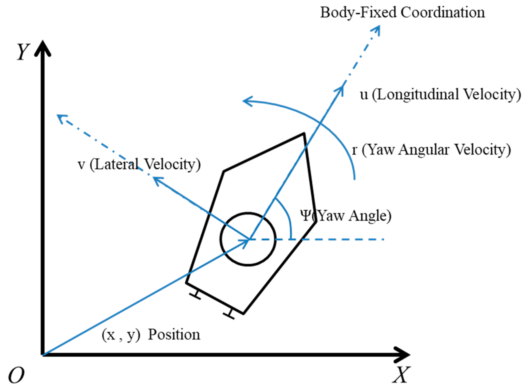
In order to simplify the problem, this paper focuses solely on the horizontal plane motion of the USV [39]. The planar motion of the USV is illustrated in Figure 2. To facilitate computer simulations of the USV motion, certain simplifications were made, which are outlined as follows:
  • Neglecting roll, pitch, and heave motion: The motion of the USV in the roll, pitch, and heave directions is disregarded for simplicity.
  • Neutral buoyancy and body-fixed coordinate: The USV is assumed to have neutral buoyancy, and the origin of the body-fixed coordinate system is positioned at the center of mass of the USV.
  • Three planes of symmetry: The USV possesses three planes of symmetry, which aid in simplifying the analysis and modeling process.
By adopting these simplifications, the focus is placed on the planar motion of the USV, allowing for more manageable simulations and analyses.

3.2. Vehicle Kinematic Model and Dynamic Model

The vessel’s kinematic model is utilized to describe its planar motion, as follows:
X ˙ = u cos ψ v sin ψ Y ˙ = u sin ψ + v cos ψ ψ ˙ = r
where u and v represent the longitudinal and lateral velocities. X is the longitudinal position, and Y is the lateral position. ψ is the yaw angle, and r is the yaw rate.
The kinematic model illustrates the correlation between the vehicle’s potion and velocity. Furthermore, the dynamic model of the USV can be expressed as
M v ˙ = τ T + τ T w C ( v ) v D ( v ) v
where M = d i a g { m 11 , m 22 , m 33 } is the inertial matrix, and D = d i a g { d 11 , d 22 , d 33 } is the damping matrix. The centripetal force matrix of the kinematic model is
C = 0 0 m 22 v 0 0 m 11 u m 22 v m 11 u 0
τ T = τ u 0 τ r contains forward thrust τ u and the yawing moment τ r . τ T w = [ τ T w u , τ T w v , τ T w r ] represents the external disturbance’s effect on [ u , v , r ] .
From the aforementioned information, the dynamic model can be written as:
u ˙ = ( τ u d 11 u + m 22 v r ) / m 11 v ˙ = ( d 22 v m 11 u r ) / m 22 r ˙ = ( τ r d 33 r m 22 u v + m 11 u v ) / m 33
where d 11 = ( X u + X u u u ) , d 22 = ( Y v + Y v v v ) , d 33 = ( N r + N r r r ) . X u , X u u , Y v , Y v v , N r , N r r are the first-order and second-order fluid coefficients, respectively.

3.3. RBF Neural Network-Based Model Predictive Control

The above part follows the classical kinematic model and dynamic model of USV. However, due to the different characteristics of each USV in practical applications, the vessel’s motion cannot be accurately described by the universal model alone.
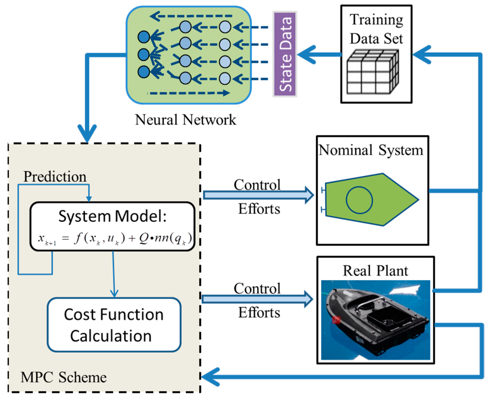
To enhance the accuracy of the vehicle model, we introduce an online learning neural network component to take the residual model uncertainty into account. This method is improved based on the measurement tools and the neural network. The main idea is shown in Figure 3.
Here, we identify an unknown function d t r u e : n z n d from a collection of inputs z k n z and outputs y k n d . Then, the considered model used for control can be expressed as:
x k + 1 = f ( x k , u k ) + Q · n n ( q k )
where f ( x k , u k ) describes the nominal vehicle dynamics, and n n · is the additional neural network part, estimating the modeling error of the nominal model mentioned above. u k = [ T l T r ] is the control efforts. The learned part n n · of the dynamics is assumed to only affect the subspace spanned by Q , corresponding to the velocity states of the vehicle. The learning part depends on a set of features q k that are relevant to the neural network.
Based on physical assumptions, we presume that the vehicle model error is mainly caused by the dynamic part of the system equations. In the following research, a learning vector was drawn into the USV model independently, as:
q = u ; v ; r ; T l ; T r
The difference between the nominal model predictions and the actual measurement state will be used as a database for online learning of the neural network, which is
y k = Q · ( x k + 1 f ( x k , u k ) ) = n n ( q k )
where Q is the Moore–Penrose pseudo-inverse, and the true modeling error function is n n ( q k ) .
Therefore, the USV path tracking control problem can be described as the following constrained dynamic optimization problem:
min J ( k ) = min i = 0 N 1 e ( k + i | k ) R 2 + u ( k + i | k ) Q 2
s . t . x k + 1 = f n o m ( x k , u k ) + Q · n n ( q k )
e ( k + 1 ) = x k + 1 x r e f
u m i n u k u m a x , k = 1 , , N c
x 0 = x k
where R is the weight matrix of the path tracking state deviation, and Q is the control input weight matrix. x k + 1 represents the model state after the compensation of the neural network. Let x r e f be the reference state. Let u k = [ T l T r ] be the control input, x 0 be the initial states of prediction and x k be the current state feedback of the real plant.
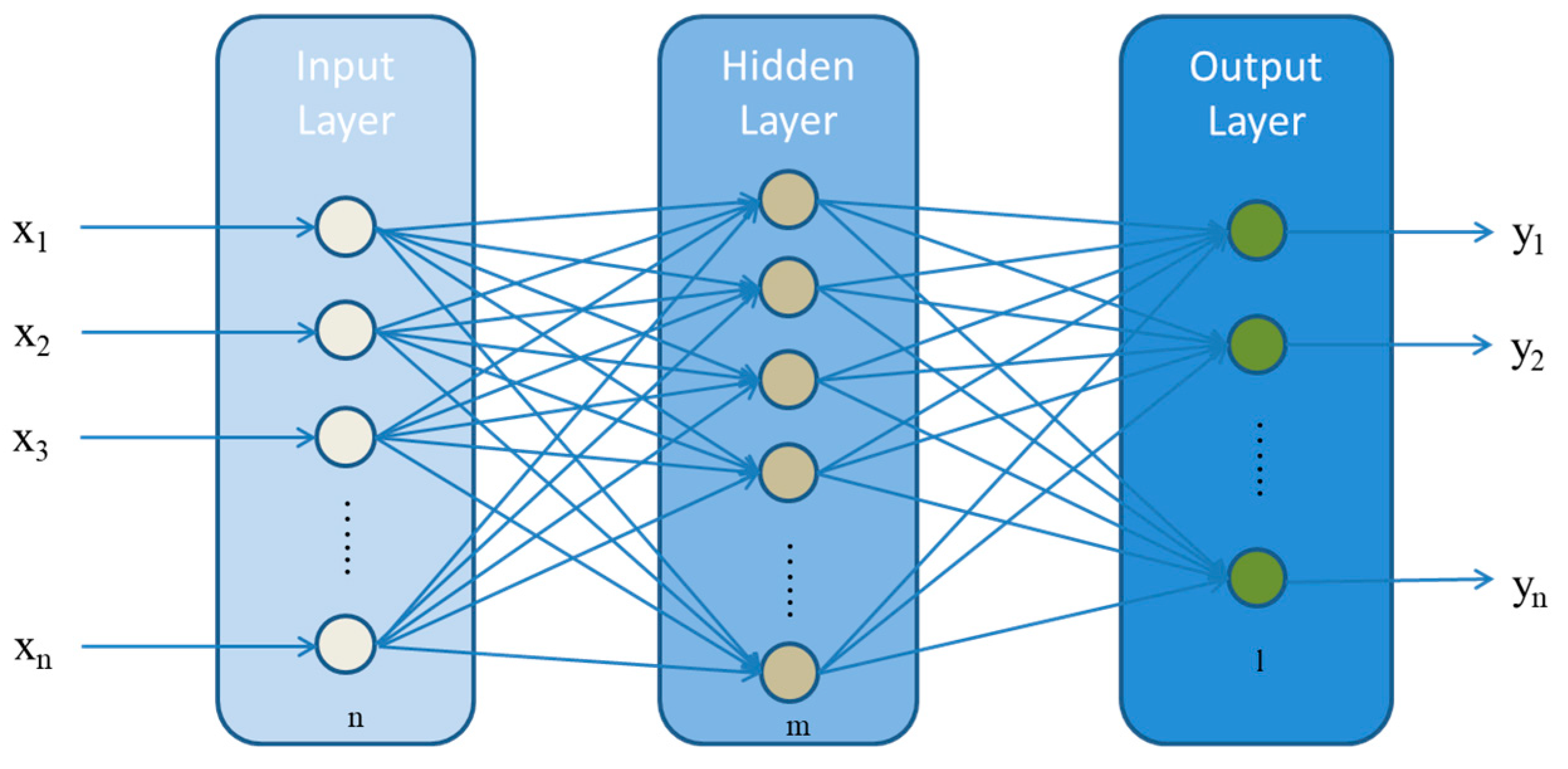
The radial basis function neural network (RBF-NNs) approximator was chosen to tackle the structural and parameter uncertainties. The structure of RBF-NNs is depicted in Figure 4, consisting of three layers: the input layer, the hidden layer and the output layer. The first layer of structure, the input layer, is expressed as X = [ x i ] Τ . This layer assigns n inputs to m nodes of the second hidden layer. The output of the second hidden layer is H = [ h j ] Τ , where x i is the i th input of the input layer, and h j is j th output of the hidden layer. In this paper, the Gaussian function is chosen as the activation function of the neural network, which is
h j ( x ) = exp x c j 2 2 σ j 2
where x c j represents the Euclidean distance between x and c j . Let c j and σ j be the center and width of the Gauss basis function.
The third output layer represents the overall output of the neural network. The prediction output of the network is calculated through a linear combination of hidden layers’ output. Thus, we obtain:
y q ( t ) = j = 1 m h w j q T = h 1 w 1 q + h 2 w 2 q + + h m w m q
where w j q represents the weight vector from the j th hidden layer node to the q th output layer node.
By combining Equation (26), the uncertainty of USV can be expressed as:
n n ( q k ) = W T H x k + ε
where W is the weight matrix from the hidden layer to the output layer. H is the vector calculated by Equation (25), and ε is the deviation term. The dimensions of the weight matrix W and H are m × l and n × m . Let n , m and l be the number of nodes in the input layer, hidden layer and output layer.

3.4. Fault-Tolerance Strategy

The studied USV is equipped with two propellers that generate the forward force. However, in the fault condition, the propellers are unable to provide the desired output torque. Thus, the USV is incapable of tracking the reference path, potentially resulting in collisions. The actuator fault is taken into account in the controller design process.
Regarding the proportional fault, the propeller torque under the faulty conditions is proportional to that of the health state. Let λ represent the fault parameter, and the torque of the propeller under the faulty condition is written as
T i f = λ T i
where Tif is the output torque of the  i   t h thruster and i = 1 , r . For the reduced output torque under the fault condition, the fault parameter λ is confined as
0 λ 1
In the fault condition, the control efforts need to be modified. Therefore, the final output of the controller is changed under consideration of the proportion case mentioned above in order to guarantee the USV’s path tracking. This can be specifically expressed as
u f = [ T h λ T f ]
Then, we substitute the above equation into Equation (21) and use the updated model, shown as Equation (31), to adaptively adjust the calculation output of MPC.
x k + 1 = f n o m ( x k , u k ) + Q · n n ( q k ) ,   u k f = [ T h λ T f ]
Furthermore, the limiting fault is considered and introduced in the following equations. The output torque is limited to a fixed value that is reduced when the fault occurs. This can be expressed as
T i max = T f a u l t max < T h max
where T f a u l t max is the maximum of the faulty thrusters’ torque, and T h max is the maximum of the healthy thrusters’ torque.
In this case, we set the maximum thrust of the faulty thruster as T i f max , as shown in the following equation:
0 < T i f T i f max < T h max
Then, we obtain Equation (34) by substituting the new thrust constraint into Equation (23), as follows:
u f m i n u k f u f m a x , k = 1 , , N c

4. Simulation Results

For the simulations, a computer with MATLAB 2019a on an Intel i7-127000 CPU with 32 GB of RAM was utilized. In order to evaluate the performance of the proposed method, we conducted a series of simulations and compared the results with those obtained from the other methods. First, the collision avoidance performance of the Kino-RRT* algorithm is shown as a comparison of the proposed algorithm. Then, we show the advantage of RBF-MPC with the fault-tolerance strategies by comparing it with the traditional MPC under faulty conditions. Furthermore, we demonstrate the well-tracking performance of the designed fault-tolerant controller for the planned path.

4.1. Collision Avoidance Path Performance Comparison in Simulation Studies

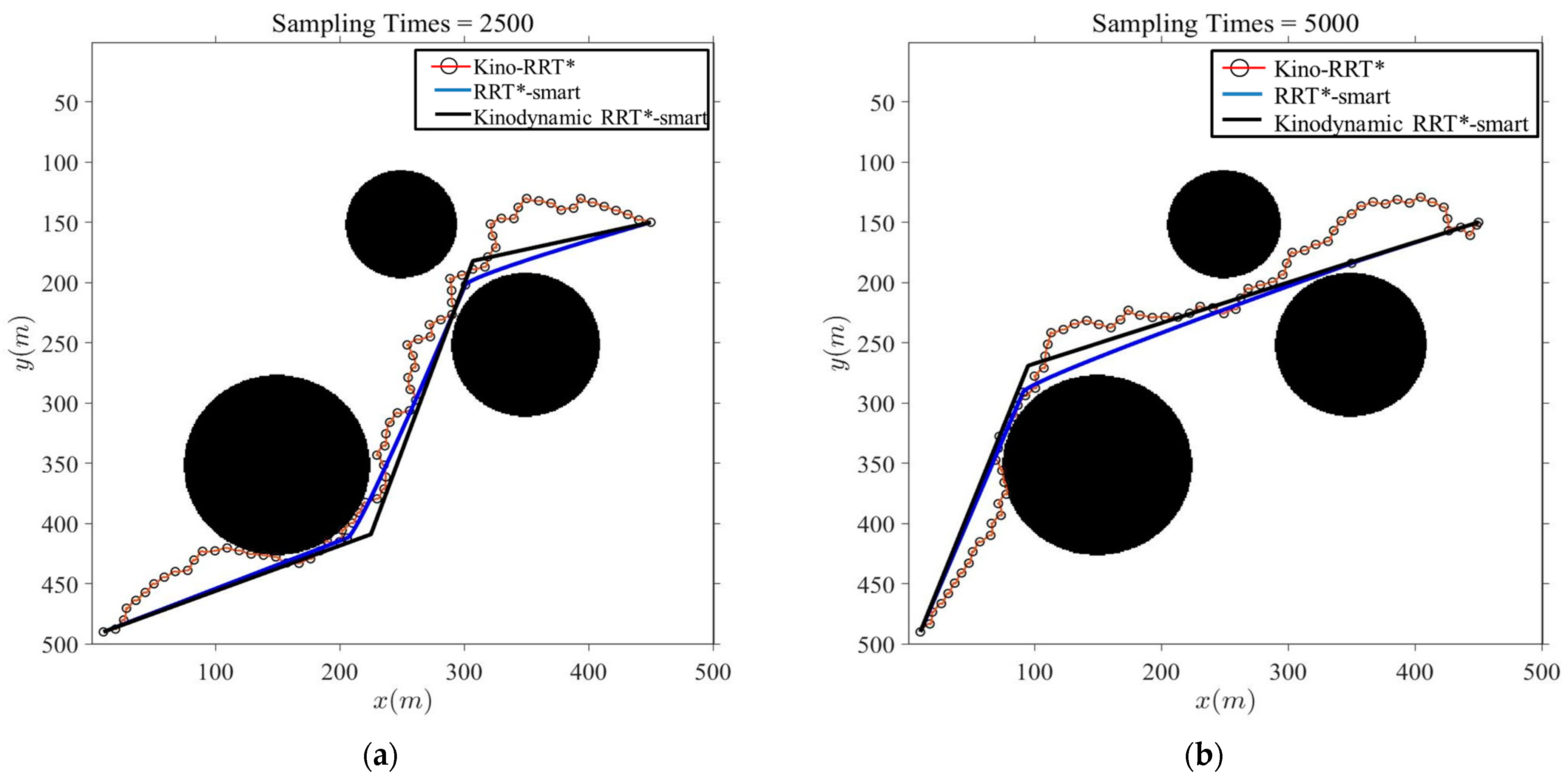
In the simulation environment, the global map is represented as a rectangular area with pixels of 500 × 500 representing an ocean area of 500 × 500 m. The obstacles are randomly set to represent floats or observation stations to be avoided. The results of the Kino-RRT* algorithm and the kinodynamic RRT*-smart algorithm are given in Figure 5. In Figure 5, we can see that the proposed algorithm found a better path under the same sampling conditions.
Furthermore, due to the unique randomness of the RRT algorithm, we conducted ten sets of simulation experiments and took their average values. The data are shown in Table 1. Upon analyzing the data, it becomes apparent that increasing the number of sampling times in the RRT algorithm leads to longer planning times. However, it also results in improved planning effectiveness. From Table 1, we can draw a conclusion that the path length is 20.48% less than Kino-RRT*’s result when the sampling times are 5000. This is because the triangular inequality concept optimizes the path cost directly. The running time is reduced by 31.34% for less TPBVP problem solving. At the same time, our biased sampling strategy also reduces the path costs via the kinodynamic constraints, and the cost is 29.59% lower than Kino-RRT*. This also resulted in a 2.98% reduction in our path length compared to RRT*-smart.
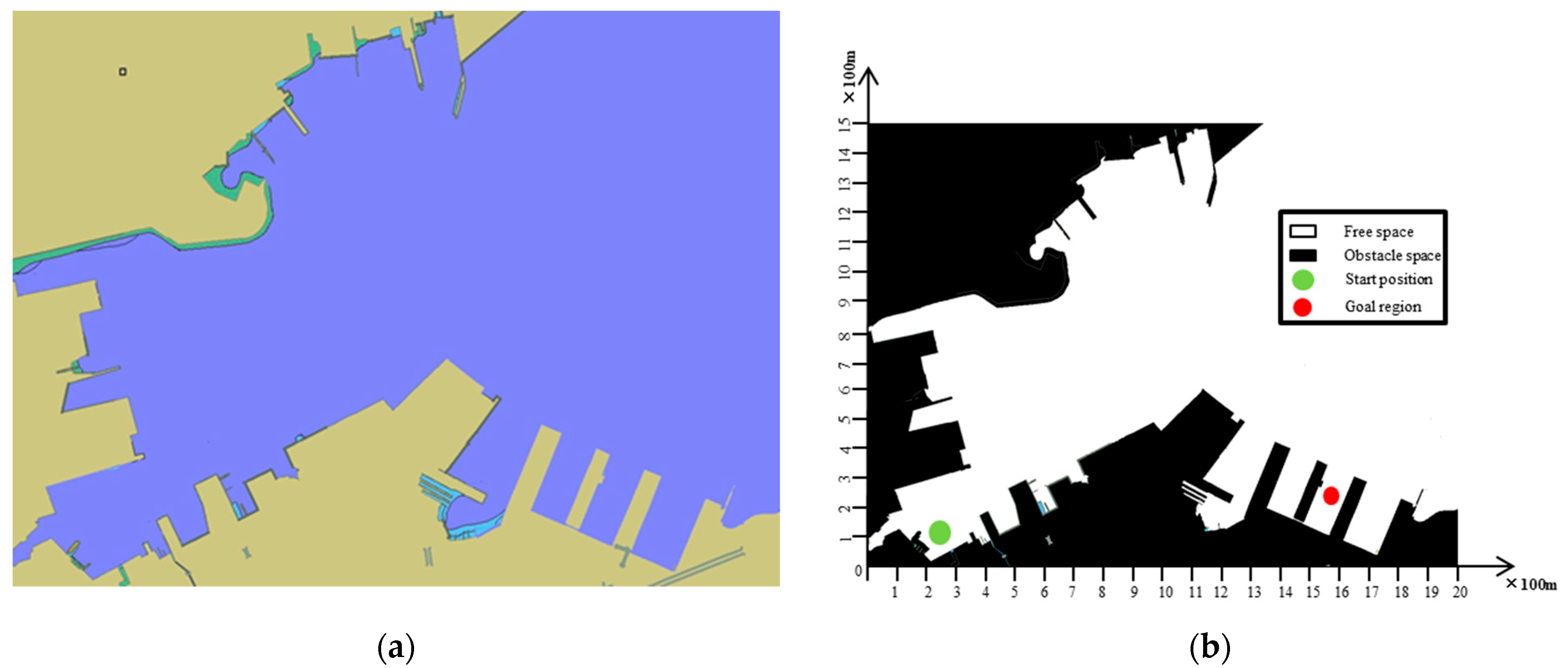
To be more practical, we chose a part of the Dalian Port image as the planning map from the Electronic Chart Display and Information System (ECDIS), as shown in Figure 6.
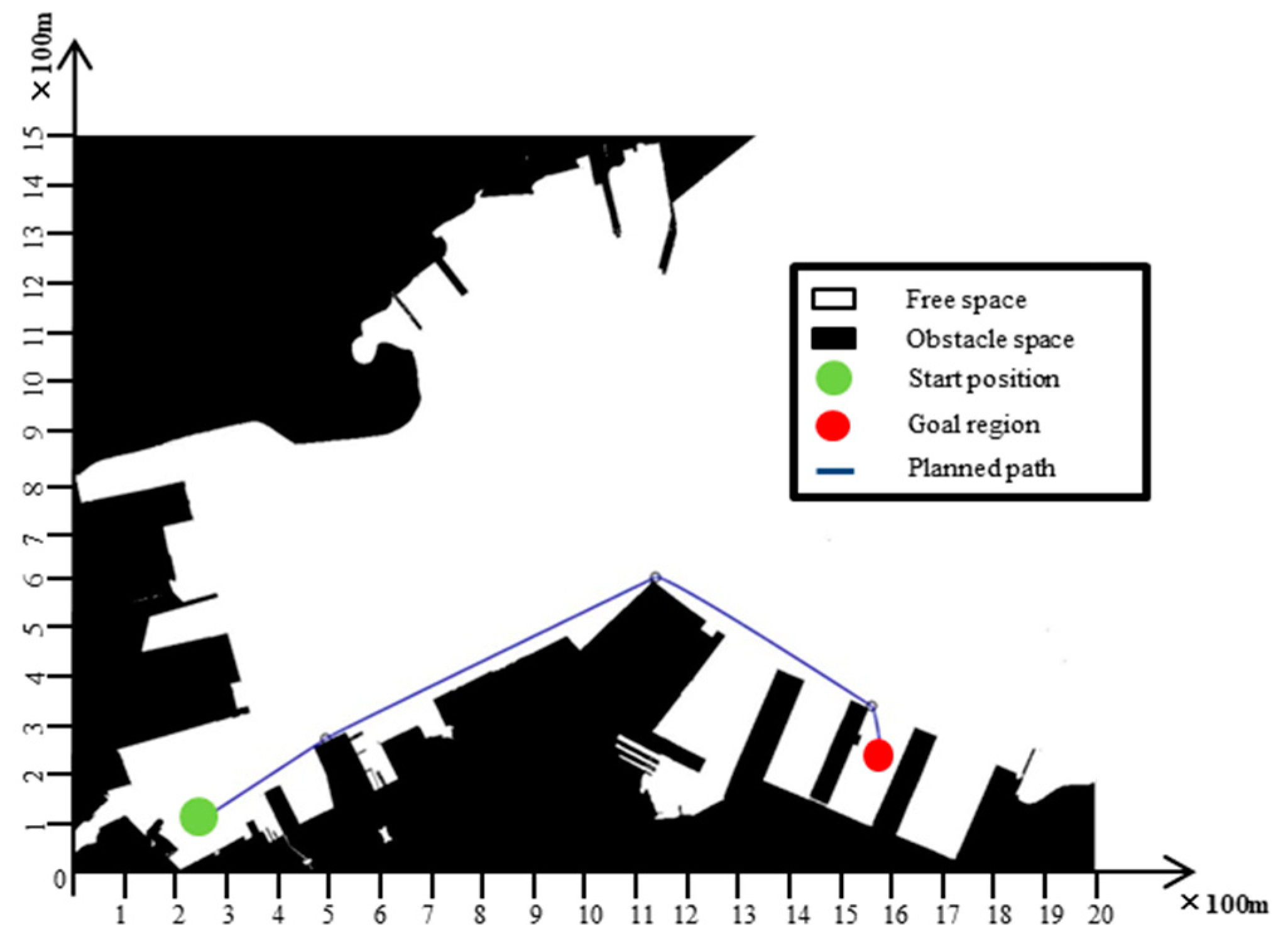
We set the initial position of the USV as [250, 100] m and the goal region as [1560, 260] m. The planning result in the real environment is shown in Figure 7.
From Figure 7, we see that the planning path is free from collisions, indicating that the proposed algorithm is capable of navigating in the actual ocean environment. As depicted in the aforementioned illustrations, we can deduce that the planning path is viable for the USV. This achievement is attributed to our incorporation of motion characteristics and kinodynamic constraints into the planning process. Consequently, the proposed algorithm is applicable for practical USV path planning.

4.2. RBF-MPC with Fault-Tolerance Strategy Performance Comparison in Simulation Studies

In order to evaluate the effectiveness of the proposed algorithm in terms of model correction and fault tolerance, comparative simulations were conducted between the proposed method and the traditional MPC. The specific kinetic parameters of the USV used in the simulations are presented in Table 2. The nominal model parameters listed in the table intentionally differ from the actual model parameters. This mismatch is performed to simulate the modeling errors that commonly exist in real-world scenarios. By introducing such modeling errors, the simulations can realistically assess the capability of the proposed algorithm to handle model inconsistencies and to provide accurate control. The external disturbance is set as
τ T w u = 3 cos ( 0.5 t ) cos ( t ) + 1.5 cos ( 0.5 t ) sin ( 0.5 t ) τ T w v = 0.6 sin ( 0.1 t ) τ T w r = 0.9 sin ( 1.1 t ) c o s ( 0.3 t )
In order to ensure the intuitive optimization effect, we chose linear path tracking for simulation. The original position of the USV was set as [0, 5] m and its original speed as [0.5, 0] m/s. In the first fault condition, the fault parameter was set as λ = 0.5 . The fault of the right thruster occurred at x = 75 m. The simulation results in the first fault case are as follows.
From Figure 8c and the locally enlarged images in Figure 8a, it can be seen that RBF-MPC can enable the USV to achieve the line tracking faster. This observation demonstrates the effectiveness of online RBF neural network learning in compensating for model errors. From Figure 8b, it can be seen that external interference has an impact on the USV yaw angle. From the local enlarged image, it can be seen that under the same interference conditions, RBF-MPC is less affected by disturbances. Therefore, we can analyze that compared to the traditional MPC, our designed RBF-MPC has stronger anti-interference ability. As shown in Figure 8b,c, after the fault occurs, the yaw angle of RBF-MPC with the fault-tolerant strategy does not change significantly, and it can still stably track the preset trajectory, but the traditional MPC cannot. This verifies the effectiveness of the fault-tolerant strategy.
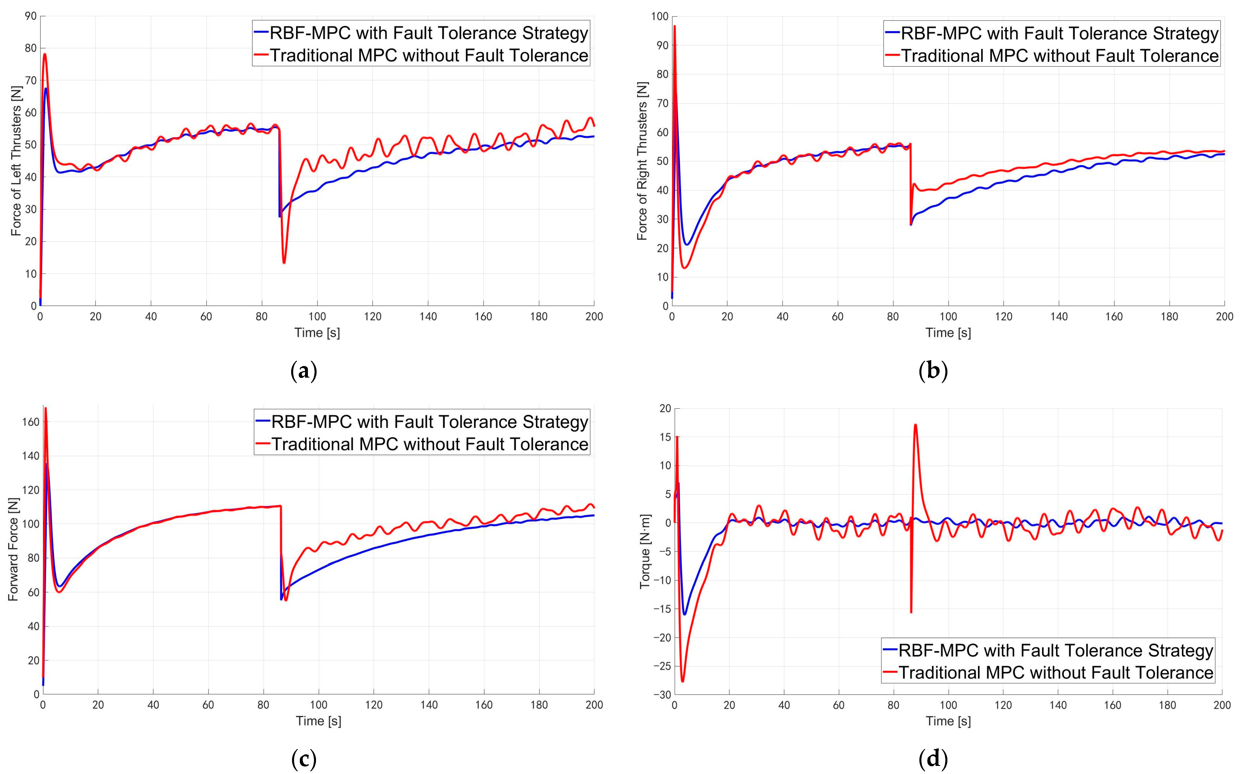
In Figure 9a, the fault tolerant strategy makes the USV’s forward speed change smoother. Figure 9b shows that the RBF-MPC with the fault-tolerant strategy can make the USV’s lateral speed converge to 0 m/s faster and changes little when the fault occurs compared with the traditional MPC. From Figure 10d, it is evident that during the initial operation stage of the USV (0–20 m), the torque variation in the computed output of RBF-MPC is smaller. By analyzing the other figures, the traditional MPC exhibits more significant changes in control output compared to RBF-MPC integrated with the fault-tolerant strategy when a fault occurs. Moreover, the traditional MPC is more susceptible to external disturbances. In Figure 11b, we can see that the real force of the right thruster is half of the MPC output, which represents the proportional failure. From Figure 10 and Figure 11, a conclusion can be drawn that the MPC with the fault-tolerant strategy can autonomously adapt to the proportional fault and adjust thrust output to ensure the normal operation of the USV.
In the second fault case, the fault parameter is set as T f max = 50   N. The fault of the right thruster occurs at x = 100   m. The simulation results of the second type of fault are as follows.
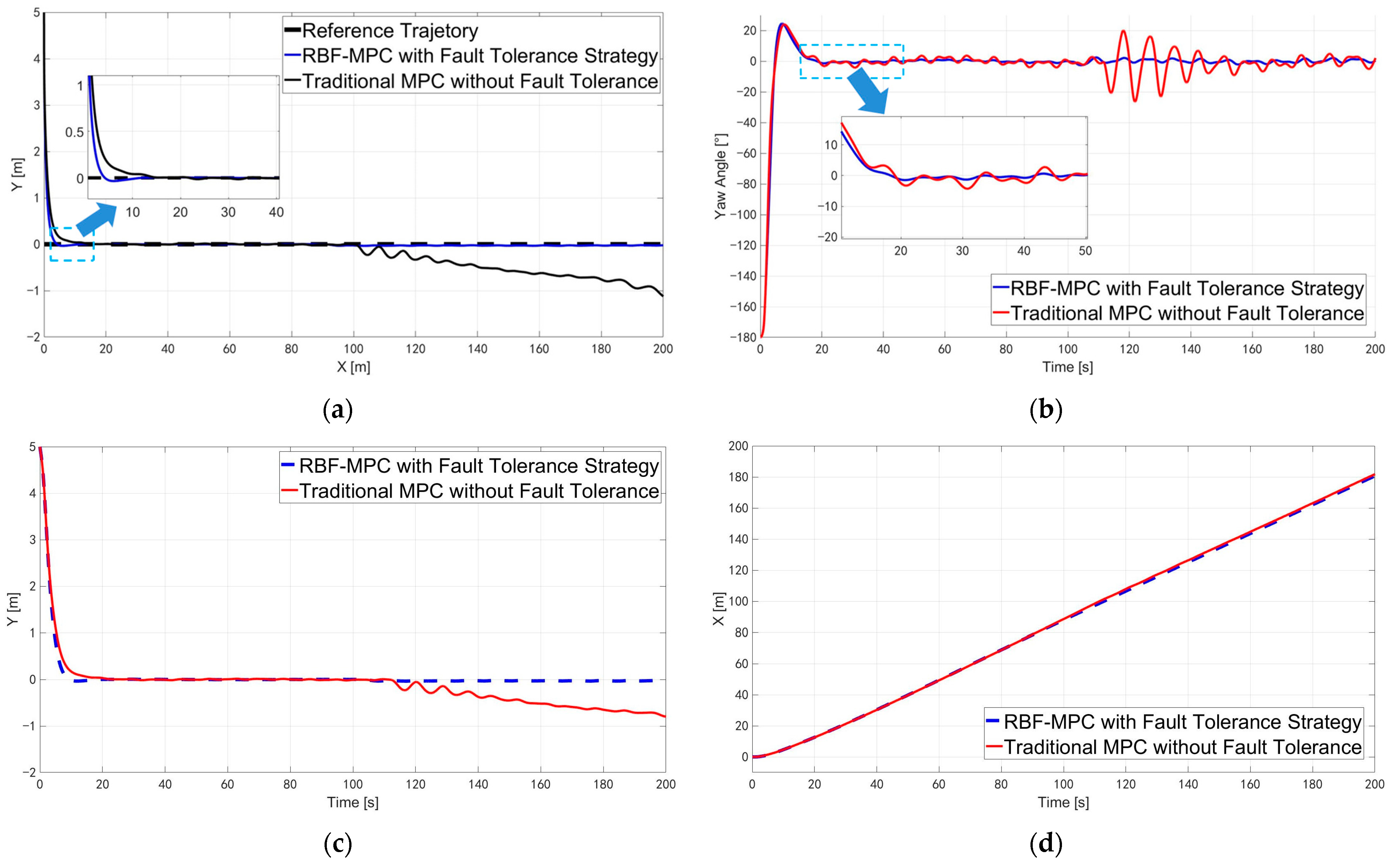
From Figure 12c and the magnified images in Figure 12a, it is evident that RBF-MPC effectively modifies the nominal model used within the MPC framework. The magnified image in Figure 12b demonstrates that the yaw angle of the USV under RBF-MPC control is less affected by external disturbances. Hence, we conclude that RBF-MPC exhibits a certain degree of disturbance attenuation. By analyzing Figure 12b–d collectively, we can deduce that after the fault occurs, the yaw angle of the USV controlled by the traditional MPC changes greatly, and the displacement in the Y direction becomes unstable. In contrast, the RBF-MPC demonstrates the effectiveness of the designed fault-tolerant strategy as it maintains relatively stable yaw angles and stable displacement even in the presence of faults. The simulation proves that when the limiting fault occurs, the MPC controller incorporating a fault-tolerant strategy enables the USV to stably track straight lines, which verifies the effectiveness of the fault-tolerant strategy for limiting faults.
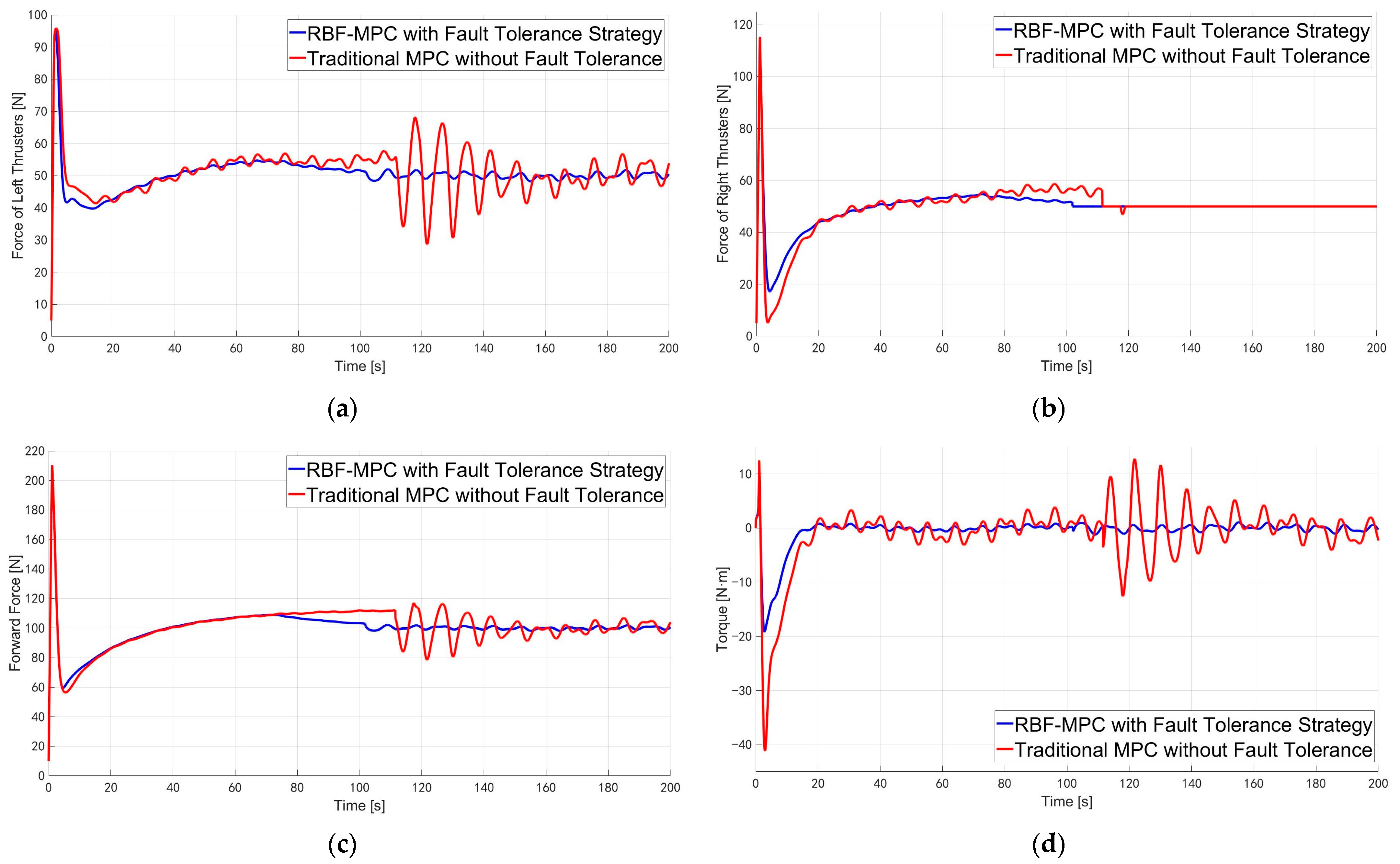
From Figure 13, it can be observed that the introduced external disturbances have an impact on both the forward velocity and longitudinal velocity, but RBF-MPC is less affected by these disturbances. Additionally, in the event of a fault, the velocity of the USV under MPC control without the fault-tolerant strategy exhibits increased oscillations. In Figure 14a,b, it can be observed that when a fault occurs in the right thruster, the thrust is constrained to 50 N. However, RBF-MPC with the fault-tolerant strategy adjusts the thrust output of the left thruster to ensure the normal operation of the USV. From Figure 14c,d, it can be deduced that RBF-MPC with the fault-tolerant strategy exhibits a small variation in thruster output after a fault occurs. However, the traditional MPC, due to the combined effect of the fault and external disturbances, fails to achieve stable control of the USV.
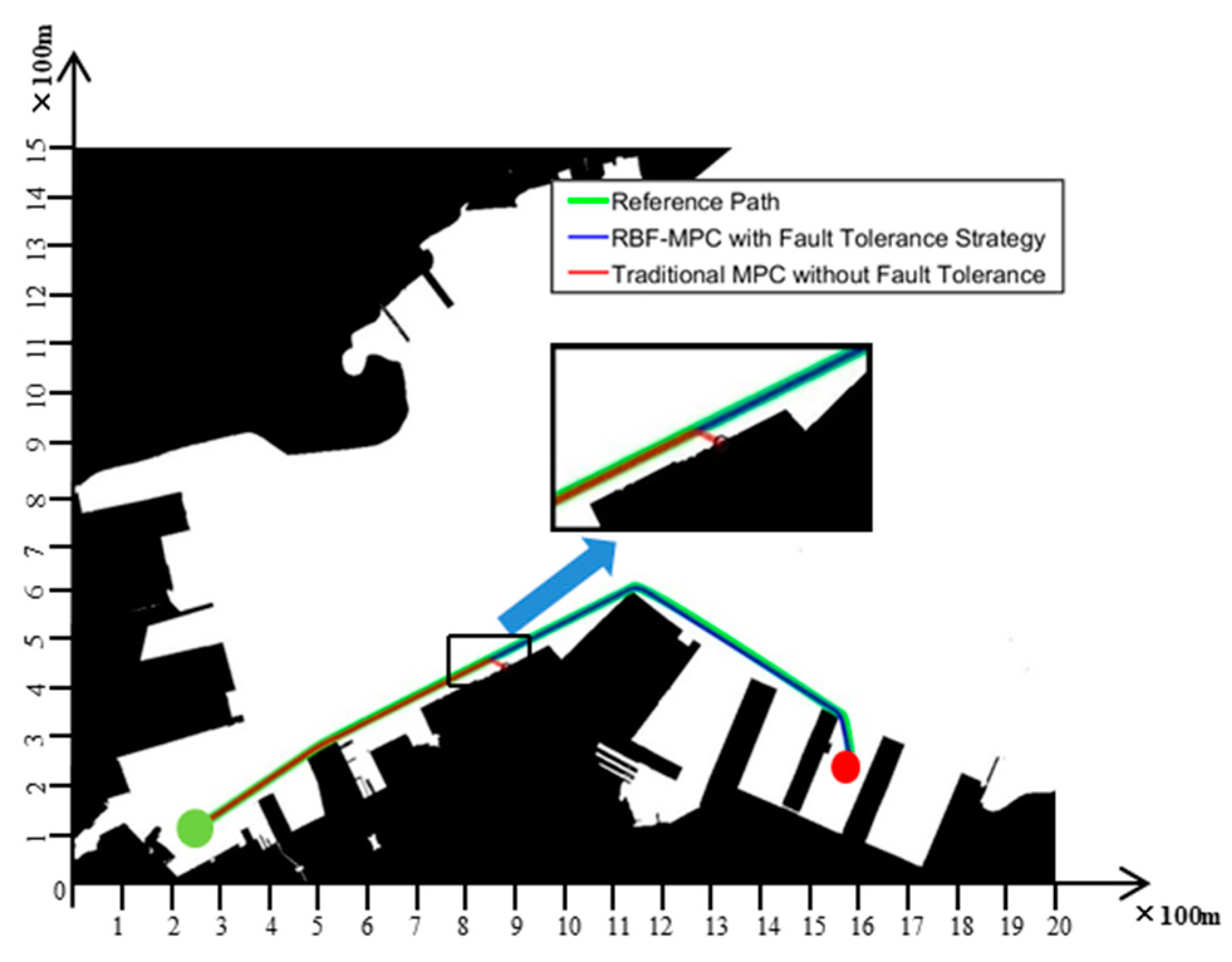
In Figure 15, the simulation illustrates that RBF-MPC with the fault-tolerant strategy makes the USV track the planned path even under the thruster-fault condition. From the partial enlarged view, the traditional MPC cannot control the USV well, and the USV collides with an obstacle when the fault occurs.
In summary, the proposed RBF-MPC combined with the fault-tolerant strategy has shown the effective performances in terms of model error correction and fault-tolerant control.

5. Conclusions

This paper focuses on two key issues in USV technology: path planning and tracking control. We developed the kinodynamic RRT*-smart algorithm and an online-learning-based MPC algorithm for the USV, considering the modeling error and actuator faults. The planning algorithm uses geometric optimization theory to optimize the paths generated by random trees in a geometric sense. Then, the optimized path points are utilized for biased sampling and generating paths that adhere to the kinodynamic constraints. Compared to the traditional methods, the proposed approach exhibits a lower computational cost for solving the optimized path. After the reference path was given, we designed the RBF-MPC scheme, which utilizes the learning ability of neural networks to approximate modeling errors. This method introduces the training results of RBF-NNs into the cost function calculation of MPC, making the nominal model used in MPC approximate the actual model, and achieving accurate control of the USV. Building upon this method, different fault-tolerant strategies were developed, taking into account the potential occurrence of thruster failures. The strategies were integrated into the RBF-MPC framework, and their effectiveness was verified by comparing them with the traditional MPC in the numerical simulation.
In our future research endeavors, we will prioritize the following issues:
(1)
Application to a USV physical platform: We aim to implement and validate the effectiveness of the proposed method on an actual USV physical platform through experimentation.
(2)
Learning-based MPC: We will develop the learning-based MPC algorithm that obviates the need for explicit fault-tolerant strategy design. By leveraging the power of neural networks, we aim to approximate the changes in the USV dynamic model induced by faults, thereby circumventing the task of fault-tolerant strategy design.
(3)
Optimization of sampling strategy: We will delve deeper into the optimization of the sampling strategy employed in our path planning algorithm. Additionally, we will try to provide evidence of the algorithm’s probability completeness and asymptotic optimality.

Author Contributions

Conceptualization, Y.S. and Y.C.; methodology, Y.S. and Y.C.; software, Y.S.; validation, J.G. and Y.W.; formal analysis, Y.W.; writing—original draft preparation, Y.S.; writing—review and editing, Y.C., J.G., Y.W. and G.P.; funding acquisition, G.P. All authors have read and agreed to the published version of the manuscript.

Funding

This work is supported by in part by the National Natural Science Foundation of China under Grants of 51979228 and 52102469, in part by the Fundamental Research Funds for the Central Universities under Grant of 3102021HHZY030007, and in part by the National Basic Scientific Research Program under Grant JCKY2019207A019.

Institutional Review Board Statement

Not applicable.

Informed Consent Statement

Not applicable.

Data Availability Statement

Not applicable.

Conflicts of Interest

The authors declare no conflict of interest.

References

  1. Zhang, M.; Liu, Z.; Cai, W.; Yan, Q. Design of Low-cost Unmanned Surface Vessel for Water Surface Cleaning. In Proceedings of the 2021 China Automation Congress (CAC), Beijing, China, 22–24 October 2021; pp. 2290–2293. [Google Scholar]
  2. Mun, A.; Long, C.; Shen, K.; An, O.; Nugroho, H.; Rusydi, M.I. Fuzzy-based Control System of Unmanned Surface Vehicle (USV) for Floating Garbage Collection. In Proceedings of the 2022 IEEE International Conference on Artificial Intelligence in Engineering and Technology (IICAIET), Kota Kinabalu, Malaysia, 13–15 September 2022; pp. 1–6. [Google Scholar]
  3. Ntakolia, C.; Lyridis, D.V. Path Planning in the Case of Swarm Unmanned Surface Vehicles for Visiting Multiple Targets. J. Mar. Sci. Eng. 2023, 11, 719. [Google Scholar] [CrossRef]
  4. Mishra, R.; Koay, T.B.; Chitre, M.; Swarup, S. Multi-USV Adaptive Exploration Using Kernel Information and Residual Variance. Front. Robot. AI 2021, 8, 1–21. [Google Scholar] [CrossRef] [PubMed]
  5. Cho, H.; Jeong, S.-K.; Ji, D.-H.; Tran, N.-H.; Vu, M.T.; Choi, H.-S. Study on Control System of Integrated Unmanned Surface Vehicle and Underwater Vehicle. Sensors 2020, 20, 2633. [Google Scholar] [CrossRef] [PubMed]
  6. Hart, P.E.; Nilsson, N.J.; Raphael, B. A Formal Basis for the Heuristic Determination of Minimum Cost Paths. IEEE Trans. Syst. Sci. Cybern. 1968, 4, 100–107. [Google Scholar] [CrossRef]
  7. Stentz, A. Optimal and efficient path planning for partially-known environments. In Proceedings of the 1994 IEEE International Conference on Robotics and Automation, San Diego, CA, USA, 8–13 May 1994; pp. 3310–3317. [Google Scholar]
  8. LaValle, S.M. Randomized Kinodynamic Planning. Int. J. Robot. Res. 2001, 20, 378–400. [Google Scholar] [CrossRef]
  9. LaValle, S.M. On the Relationship Between Classical Grid Search and Probabilistic Roadmaps. Int. J. Robot. Res. 2004, 23, 673–692. [Google Scholar] [CrossRef]
  10. Karaman, S.; Frazzoli, E. Sampling-based Algorithms for Optimal Motion Planning. Int. J. Robot. Res. 2011, 30, 846–894. [Google Scholar] [CrossRef]
  11. Webb, D.J.; Berg, J. Kinodynamic RRT*: Asymptotically optimal motion planning for robots with linear dynamics. In Proceedings of the 2013 IEEE International Conference on Robotics and Automation, Karlsruhe, Germany, 6–10 May 2013; pp. 5054–5061. [Google Scholar]
  12. Li, Y.; Littlefield, Z.; Bekris, K.E. Asymptotically Optimal Sampling-based Kinodynamic Planning. Int. J. Robot. Res. 2016, 35, 528–564. [Google Scholar] [CrossRef]
  13. Li, Y.; Cui, R.; Li, Z.; Xu, D. Neural Network Approximation Based Near-Optimal Motion Planning with Kinodynamic Constraints Using RRT. IEEE Trans. Ind. Electron. 2018, 65, 8718–8729. [Google Scholar] [CrossRef]
  14. Zheng, D.; Tsiotras, P. Accelerating Kinodynamic RRT* Through Dimensionality Reduction. In Proceedings of the 2021 IEEE/RSJ International Conference on Intelligent Robots and Systems (IROS), Prague, Czech Republic, 27 September–October 2021; pp. 3674–3680. [Google Scholar]
  15. Mao, S.; Yang, P.; Gao, D.; Bao, C.; Wang, Z. A Motion Planning Method for Unmanned Surface Vehicle Based on Improved RRT Algorithm. J. Mar. Sci. Eng. 2023, 11, 687. [Google Scholar] [CrossRef]
  16. Wen, N.; Zhang, R.; Liu, G. Online planning low-cost paths for unmanned surface vehicles based on the artificial vector field and environmental heuristics. Int. J. Adv. Robot. Sys. 2020, 17, 846–894. [Google Scholar] [CrossRef]
  17. Wen, N.; Zhang, R.; Wu, J. Online planning for relative optimal and safe paths for USVs using a dual sampling domain reduction-based RRT* method. Int. J. Mach. Learn. Cyber. 2020, 11, 2665–2687. [Google Scholar] [CrossRef]
  18. Han, S.; Wang, Y.; Wang, L.; He, H. Automatic berthing for an underactuated unmanned surface vehicle: A real-time motion planning approach. Ocean Eng. 2021, 235, 109352. [Google Scholar] [CrossRef]
  19. Esfahani, H.N.; Szlapczynski, R. Model Predictive Super-Twisting Sliding Mode Control for an Autonomous Surface Vehicle. Polish Mar. Res. 2019, 26, 163–171. [Google Scholar] [CrossRef]
  20. Liang, X.; Qu, X.; Hou, Y.; Li, Y.; Zhang, R. Distributed coordinated tracking control of multiple unmanned surface vehicles under complex marine environments. Ocean Eng. 2020, 205, 107328. [Google Scholar] [CrossRef]
  21. Qu, X.; Liang, X.; Hou, Y. Fuzzy State Observer-Based Cooperative Path-Following Control of Autonomous Underwater Vehicles with Unknown Dynamics and Ocean Disturbances. Int. J. Fuzzy Syst. 2021, 23, 1849–1859. [Google Scholar] [CrossRef]
  22. Kabzan, J.; Hewing, L.; Liniger, A.; Zeilinger, M.N. Learning-Based Model Predictive Control for Autonomous Racing. IEEE Robot. Autom. Lett. 2019, 4, 3363–3370. [Google Scholar] [CrossRef]
  23. Vu, M.T.; Le, T.-H.; Thanh, H.L.N.N.; Huynh, T.-T.; Van, M.; Hoang, Q.-D.; Do, T.D. Robust Position Control of an Over-actuated Underwater Vehicle under Model Uncertainties and Ocean Current Effects Using Dynamic Sliding Mode Surface and Optimal Allocation Control. Sensors 2021, 21, 747. [Google Scholar] [CrossRef]
  24. Ning, C.; You, F. Online learning based risk-averse stochastic MPC of constrained linear uncertain systems. Automatica 2021, 125, 109402. [Google Scholar] [CrossRef]
  25. Xia, L.; Shao, C.; Li, H.; Cui, Y. Robust Model-based Reinforcement Learning USV System Guided by Lyapunov Neural Networks. In Proceedings of the 2022 IEEE International Conference on Robotics and Biomimetics (ROBIO), Jinghong, China, 5–9 December 2022; pp. 1976–1981. [Google Scholar]
  26. Shen, H.; Lv, Y.; Zhou, J.; Wang, L. An Online Parameter Estimation Method Based on Adaptive Unscented Kalman Filter for Unmanned Surface Vessel. In Proceedings of the 2022 34th Chinese Control and Decision Conference (CCDC), Hefei, China, 15–17 August 2022; pp. 2584–2589. [Google Scholar]
  27. Qu, X.; Liang, X.; Hou, Y. Path-following control of unmanned surface vehicles with unknown dynamics and unmeasured velocities. J. Mar. Sci. Technol. 2021, 26, 395–407. [Google Scholar] [CrossRef]
  28. Choo, K.-B.; Cho, H.; Park, J.-H.; Huang, J.; Jung, D.; Lee, J.; Jeong, S.-K.; Yoon, J.; Choo, J.; Choi, H.-S. A Research on Fault Diagnosis of a USV Thruster Based on PCA and Entropy. Appl. Sci. 2023, 13, 3344. [Google Scholar] [CrossRef]
  29. Yu, X.; Hao, L.; Wang, X. Fault Tolerant Control for an Unmanned Surface Vessel Based on Integral Sliding Mode State Feedback Control. Int. J. Control Autom. Syst. 2022, 20, 2514–2522. [Google Scholar] [CrossRef]
  30. Tanakitkorn, K.; Phoemsapthawee, S. Impacts of thruster configurations on the task performance of an unmanned surface vehicle. Ocean Eng. 2022, 256, 111465. [Google Scholar] [CrossRef]
  31. Wang, Y.; Jiang, B.; Wu, Z.-G.; Xie, S.; Peng, Y. Adaptive Sliding Mode Fault-Tolerant Fuzzy Tracking Control with Application to Unmanned Marine Vehicles. IEEE Trans. Syst. Man Cybern. 2021, 51, 6691–6700. [Google Scholar] [CrossRef]
  32. Guo, W.; Lin, X.; Wang, Y. Predictive Fault-tolerant Control for Trajectory Tracking of Unmanned Surface Vehicle. In Proceedings of the 2021 CAA Symposium on Fault Detection, Supervision, and Safety for Technical Processes (SAFEPROCESS), Chengdu, China, 17–18 December 2021; pp. 1–6. [Google Scholar]
  33. Ding, X.; Zhu, D.; Yan, M. Research on static fault-tolerant control method of thruster based on MPC. J. Mar. Sci. Technol. 2021, 26, 861–871. [Google Scholar] [CrossRef]
  34. Zhang, G.; Chu, S.; Zhang, W.; Liu, C. Adaptive Neural Fault-Tolerant Control for USV With the Output-Based Triggering Approach. IEEE Trans. Veh. Technol. 2022, 71, 6948–6957. [Google Scholar] [CrossRef]
  35. Nan, F.; Sun, S.; Foehn, P.; Scaramuzza, D. Nonlinear MPC for Quadrotor Fault-Tolerant Control. IEEE Robot. Autom. Lett. 2022, 7, 5047–5054. [Google Scholar] [CrossRef]
  36. Chen, Y.; Wang, J. In-Wheel-Motor-Driven Electric Vehicles Motion Control Methods Considering Motor Thermal Protection. J. Dyn. Syst. Meas. Control 2019, 141, 011015. [Google Scholar] [CrossRef]
  37. Nasir, J.; Islam, F.; Malik, U. RRT*-Smart: A rapid convergence implementation of RRT*. Int. J. Adv. Robot. Syst. 2013, 10, 299–310. [Google Scholar] [CrossRef]
  38. Chi, W.; Wang, C.; Wang, J.; Meng, M.Q.-H. Risk-DTRRT-Based Optimal Motion Planning Algorithm for Mobile Robots. IEEE Trans. Autom. Sci. Eng. 2019, 16, 1271–1288. [Google Scholar] [CrossRef]
  39. Vu, M.T.; Van, M.; Bui, D.H.P.; Do, Q.T.; Huynh, T.-T.; Lee, S.-D.; Choi, H.-S. Study on Dynamic Behavior of Unmanned Surface Vehicle-Linked Unmanned Underwater Vehicle System for Underwater Exploration. Sensors 2020, 20, 1329. [Google Scholar] [CrossRef] [PubMed]
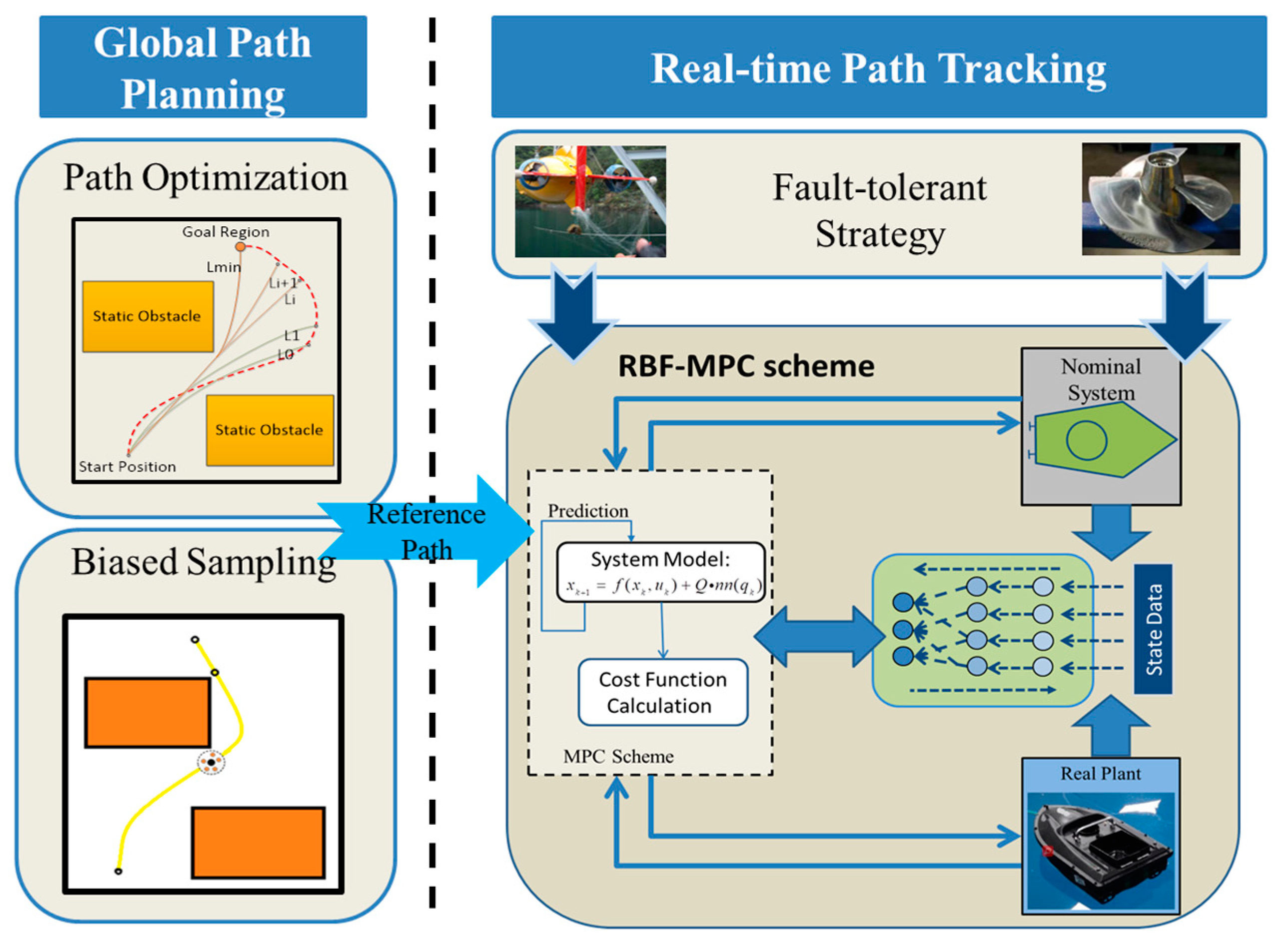
Figure 1. The proposed obstacle avoidance strategy.
Jmse 11 01107 g001
Figure 2. Vessel motion system.
Jmse 11 01107 g002
Figure 3. Architecture of NN-MPC.
Jmse 11 01107 g003
Figure 4. RBF-NN structure.
Jmse 11 01107 g004
Figure 5. Planning simulation results: (a) sampling times = 2500; (b) sampling times = 5000.
Jmse 11 01107 g005
Figure 6. Conversion from the ECDIS image to the binarization map: (a) Dalian Port partial (location: 38°57′ N, 121°38′ E, width: 2000 m, height: 1500 m); (b) binarization map.
Jmse 11 01107 g006
Figure 7. The planning path in a real environment.
Jmse 11 01107 g007
Figure 8. Trajectory tracking result in the first fault case. (a) position; (b) yaw angle; (c) X-direction displacement; (d) Y-direction displacement.
Jmse 11 01107 g008aJmse 11 01107 g008b
Figure 9. The speed of USV in the first fault case: (a) forward speed; (b) lateral speed.
Jmse 11 01107 g009
Figure 10. The force of the thrusters in the first fault case: (a) left thruster; (b) right thruster; (c) forward force; (d) torque.
Jmse 11 01107 g010
Figure 11. MPC output and real control effort in the first fault case: (a) left thruster; (b) right thruster.
Jmse 11 01107 g011
Figure 12. Trajectory tracking result in the second fault case. (a) position; (b) yaw angle; (c) X-direction displacement; (d)Y-direction displacement.
Jmse 11 01107 g012
Figure 13. The speed of the USV in the second fault case: (a) forward speed; (b) lateral speed.
Jmse 11 01107 g013
Figure 14. The force of the thrusters in the second fault case: (a) left thruster; (b) right thruster; (c) forward force; (d) torque.
Jmse 11 01107 g014
Figure 15. The planned path tracking result.
Jmse 11 01107 g015
Table 1. Summary of comparative analysis.
Sampling
Times
AlgorithmRunning
Time
Path
Cost
Path
Length
2500RRT*-smart0.45×608.73
Kino-RRT*0.67748.65752.49
proposed method0.56534.57612.31
5000RRT*-smart0.63×572.46
Kino-RRT*1.34647.55698.65
proposed method0.92455.93555.58
Table 2. The parameters of the nominal model and real plant.
Parameter m 11 m 22 m 33 X u X u u Y v Y v v N r N r r
Nominal Model141.85197.7515.6−45.6−67.26−29.54−73.85−10.71−5.59
Real Plant153.65204.3518.2−40.3−67.26−30.54−70.25−10.71−5.59
Disclaimer/Publisher’s Note: The statements, opinions and data contained in all publications are solely those of the individual author(s) and contributor(s) and not of MDPI and/or the editor(s). MDPI and/or the editor(s) disclaim responsibility for any injury to people or property resulting from any ideas, methods, instructions or products referred to in the content.