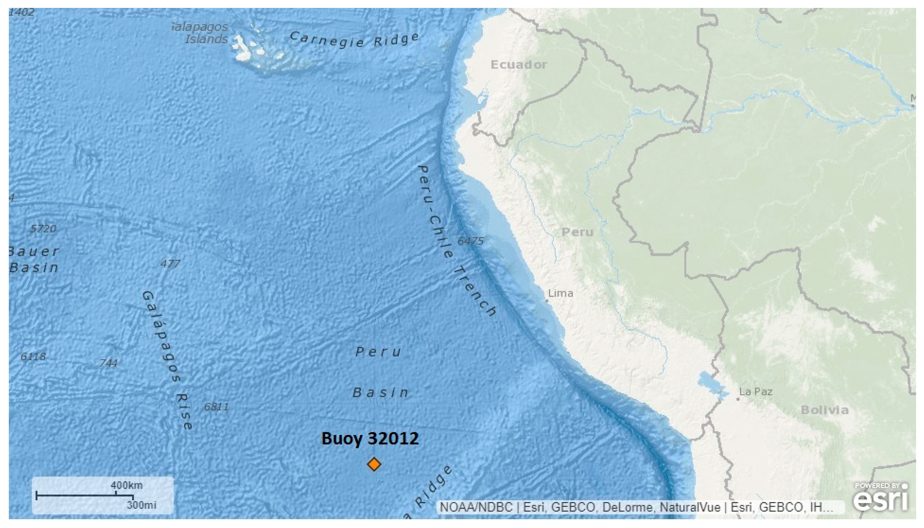
Figure 1.
Location of Buoy 32012 in the Peru Basin. The figure is taken from NDBC [
26].
Figure 1.
Location of Buoy 32012 in the Peru Basin. The figure is taken from NDBC [
26].
Figure 2.
Time series of the energy period calculated based on spectral data from Buoy 32012 in the Peru Basin.
Figure 2.
Time series of the energy period calculated based on spectral data from Buoy 32012 in the Peru Basin.
Figure 3.
Time series of the zero-up-crossing period calculated based on spectral data from Buoy 32012 in the Peru Basin.
Figure 3.
Time series of the zero-up-crossing period calculated based on spectral data from Buoy 32012 in the Peru Basin.
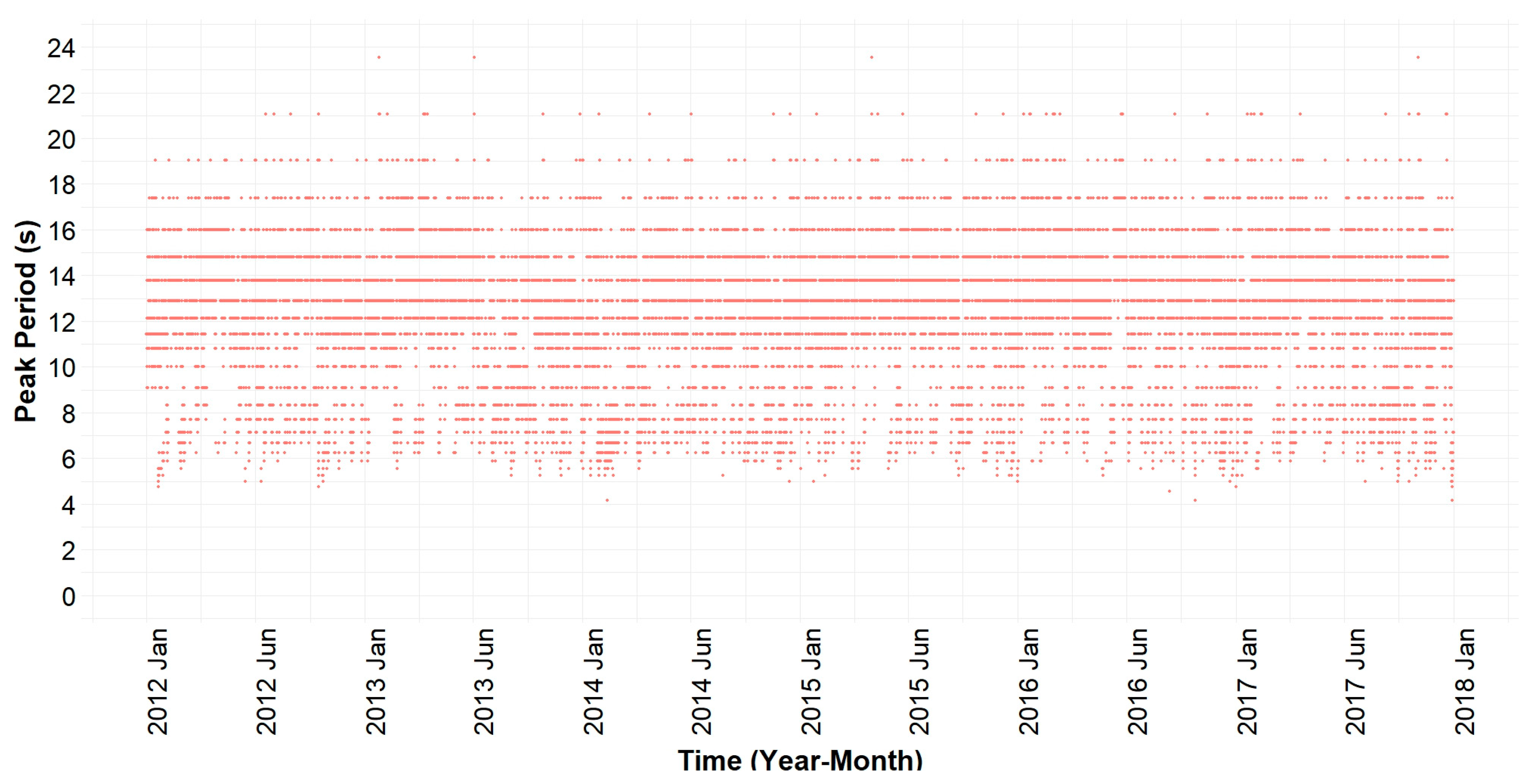
Figure 4.
Time series of the peak period taken from the sea state wave spectrums of Buoy 32012 in the Peru Basin.
Figure 4.
Time series of the peak period taken from the sea state wave spectrums of Buoy 32012 in the Peru Basin.
Figure 5.
Scatter plot of energy period, spectral data versus Bretschneider Tz, from Buoy 32012 in the Peru Basin.
Figure 5.
Scatter plot of energy period, spectral data versus Bretschneider Tz, from Buoy 32012 in the Peru Basin.
Figure 6.
Approximation error of Bretschneider Tz energy period from Buoy 32012 in the Peru Basin.
Figure 6.
Approximation error of Bretschneider Tz energy period from Buoy 32012 in the Peru Basin.
Figure 7.
Scatter plot of energy period, spectral data versus NCC Tz, from Buoy 32012 in the Peru Basin.
Figure 7.
Scatter plot of energy period, spectral data versus NCC Tz, from Buoy 32012 in the Peru Basin.
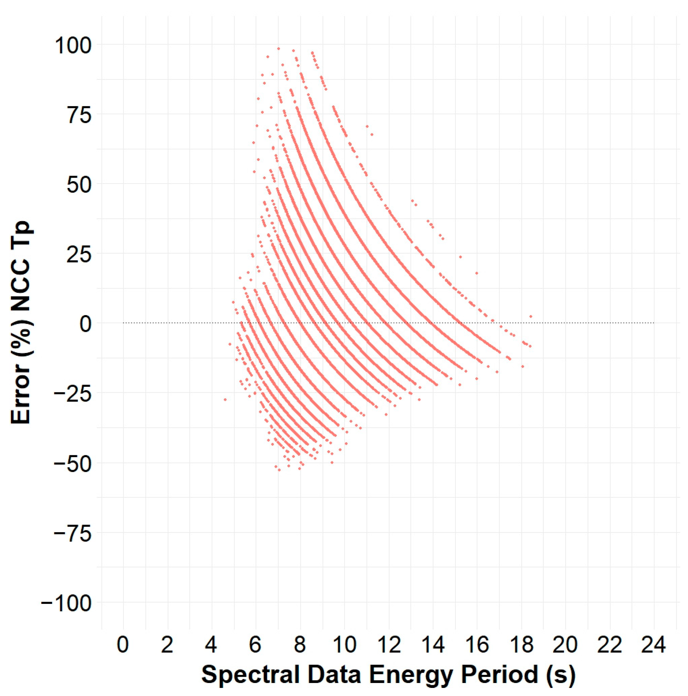
Figure 8.
Approximation error of NCC Tz energy period from Buoy 32012 in the Peru Basin.
Figure 8.
Approximation error of NCC Tz energy period from Buoy 32012 in the Peru Basin.
Figure 9.
Scatter plot of energy period, spectral data versus NCC Tp, from Buoy 32012 in the Peru Basin.
Figure 9.
Scatter plot of energy period, spectral data versus NCC Tp, from Buoy 32012 in the Peru Basin.
Figure 10.
Approximation error of NCC Tp energy period from Buoy 32012 in the Peru Basin.
Figure 10.
Approximation error of NCC Tp energy period from Buoy 32012 in the Peru Basin.
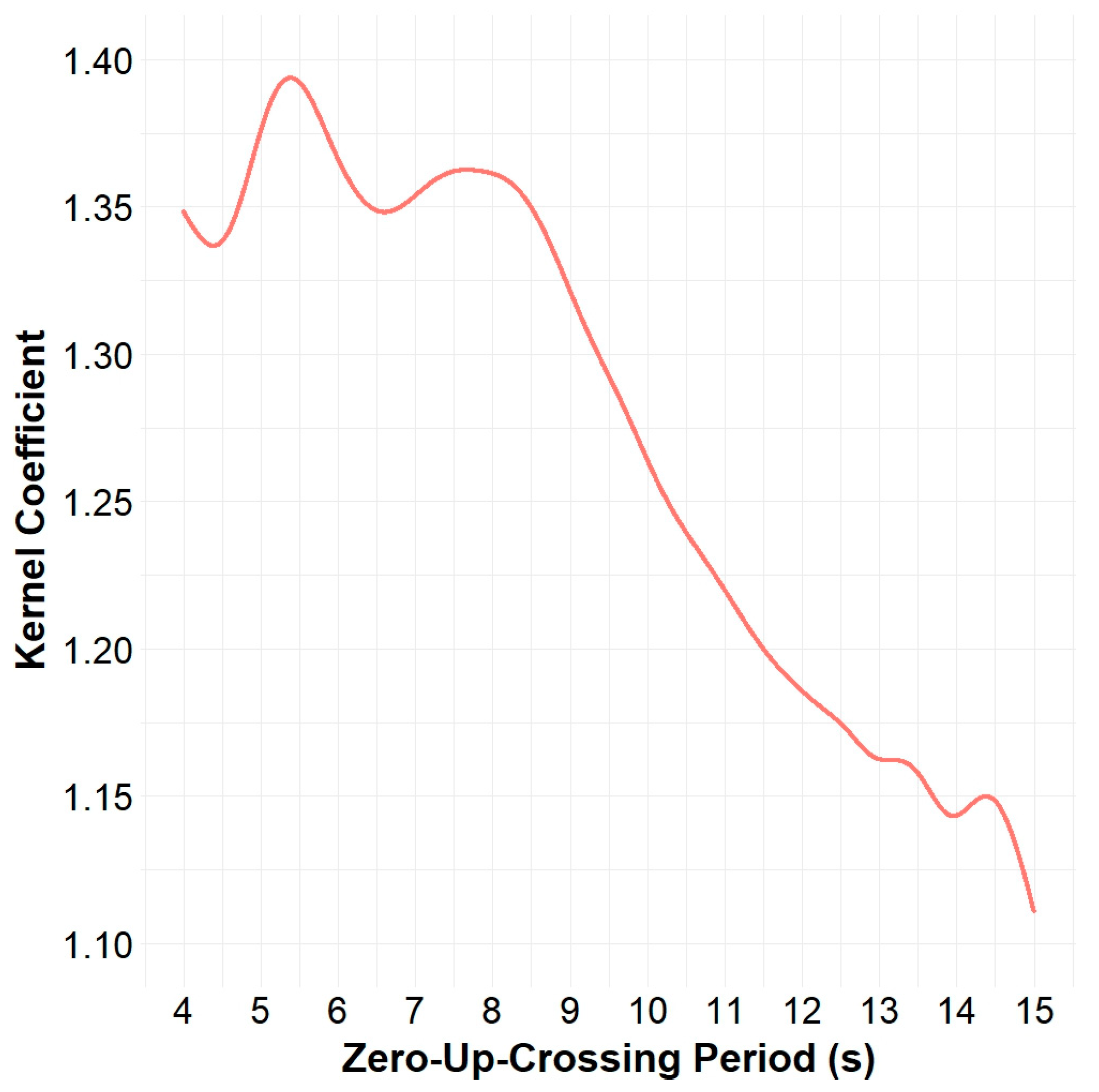
Figure 11.
The Kernel “coefficient” curve for the Peru Basin.
Figure 11.
The Kernel “coefficient” curve for the Peru Basin.
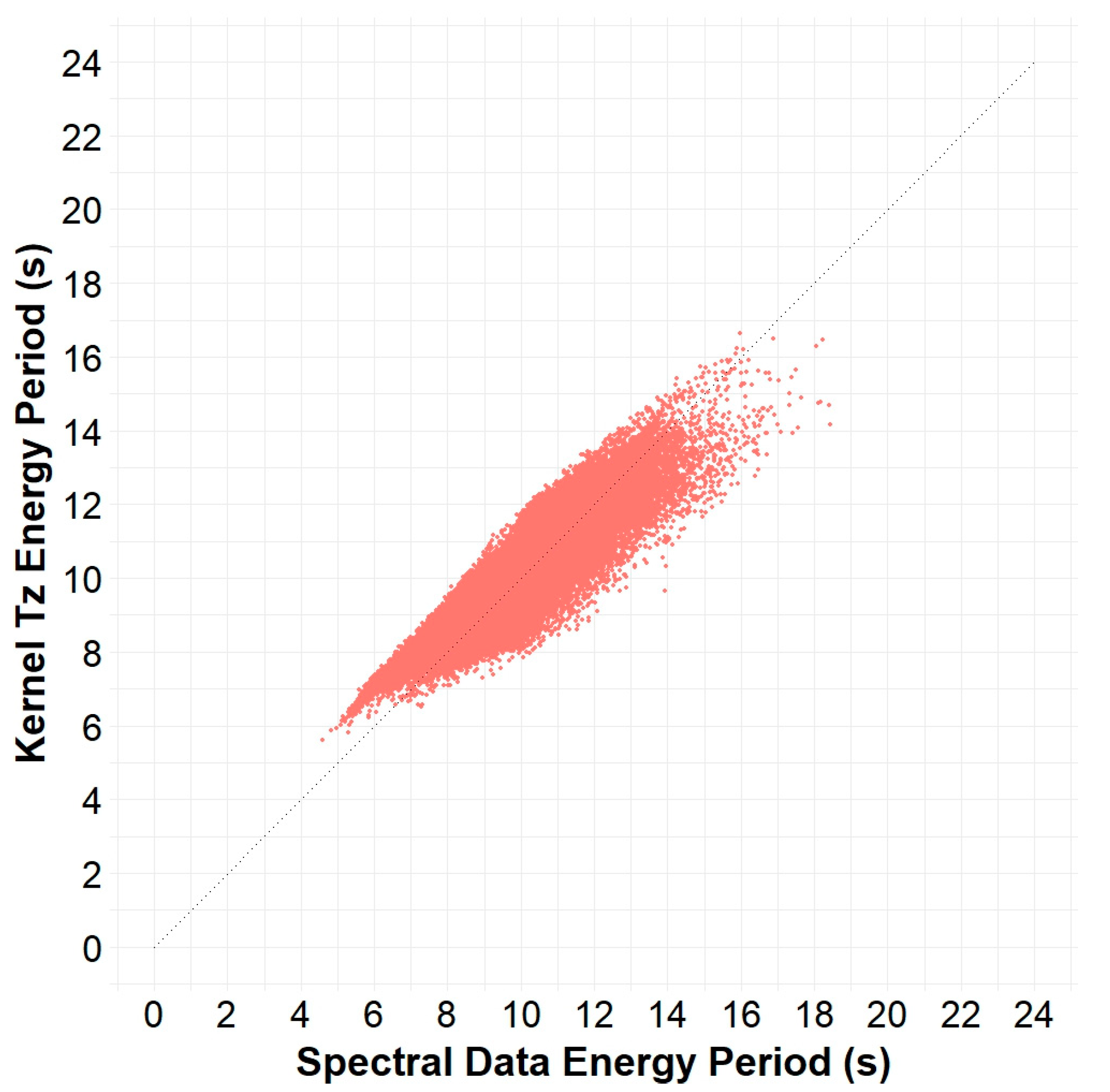
Figure 12.
Scatter plot of energy period, spectral data versus Kernel Tz, from Buoy 32012 in the Peru Basin.
Figure 12.
Scatter plot of energy period, spectral data versus Kernel Tz, from Buoy 32012 in the Peru Basin.
Figure 13.
Approximation error of Kernel Tz energy period from Buoy 32012 in the Peru Basin.
Figure 13.
Approximation error of Kernel Tz energy period from Buoy 32012 in the Peru Basin.
Figure 14.
Monthly average of the energy period, standard deviation (blue) and coefficient of variation using spectral data from Buoy 32012 in the Peru Basin. Numerical values are at the top, and CV is in brackets.
Figure 14.
Monthly average of the energy period, standard deviation (blue) and coefficient of variation using spectral data from Buoy 32012 in the Peru Basin. Numerical values are at the top, and CV is in brackets.
Figure 15.
Error percentage in calculating the monthly average of energy period using the diverse approximations.
Figure 15.
Error percentage in calculating the monthly average of energy period using the diverse approximations.
Figure 16.
Error percentage in calculating the monthly average of coefficient of variation using the diverse approximations.
Figure 16.
Error percentage in calculating the monthly average of coefficient of variation using the diverse approximations.
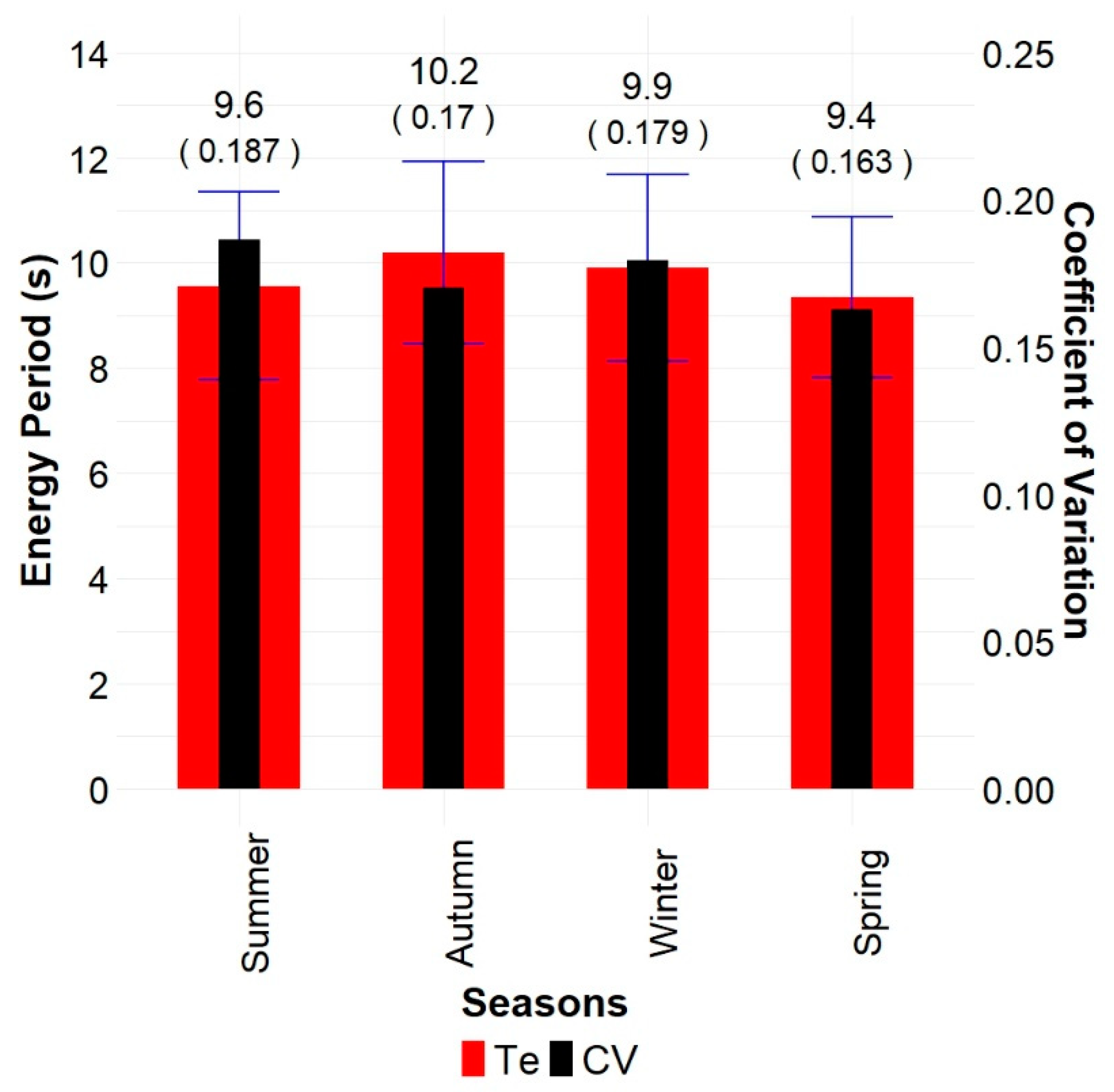
Figure 17.
Seasonal average of energy period, standard deviation (blue) and coefficient of variation using spectral data from Buoy 32012 in the Peru Basin. Numerical values are at the top, and CV is in brackets.
Figure 17.
Seasonal average of energy period, standard deviation (blue) and coefficient of variation using spectral data from Buoy 32012 in the Peru Basin. Numerical values are at the top, and CV is in brackets.
Figure 18.
Error percentage in calculating the seasonal average of energy period using the diverse approximations.
Figure 18.
Error percentage in calculating the seasonal average of energy period using the diverse approximations.
Figure 19.
Error percentages in calculating the seasonal average of coefficient of variation using the diverse approximations.
Figure 19.
Error percentages in calculating the seasonal average of coefficient of variation using the diverse approximations.
Table 1.
Ocean Buoy 32012 deployed in the Peru Basin, providing historical data.
Table 1.
Ocean Buoy 32012 deployed in the Peru Basin, providing historical data.
| Buoy | Latitude (° S) | Longitude (° W) | Sea Depth (m) |
|---|
| 32012 | 19.425 | 85.078 | 4524 |
Table 2.
Maximum percentage error generated by each of the diverse approximations of Te. The table also presents the Te estimated and the date and time of occurrence taken from the spectral data of Buoy 32012 in the Peru Basin.
Table 2.
Maximum percentage error generated by each of the diverse approximations of Te. The table also presents the Te estimated and the date and time of occurrence taken from the spectral data of Buoy 32012 in the Peru Basin.
| Approximation | Maximum | Spectral | When |
|---|
| Error (%) | Te (s) | DD/MM/YEAR HH:MM |
|---|
| Kernel Tz | −30.6 | 13.9 | 02/11/2017 14:00 |
| NCC Tz | −36.0 | 13.9 | 02/11/2017 14:00 |
| Bretschneider Tz | −38.6 | 13.9 | 02/11/2017 14:00 |
| NCC Tp | 98.4 | 7.0 | 29/12/2017 04:00 |
| Bretschneider Tp | 112.5 | 7.0 | 29/12/2017 04:00 |
| JONSWAP Tp | 120.7 | 7.0 | 29/12/2017 04:00 |
Table 3.
Annual average, extreme values and error percentage from calculating the monthly average of energy period using spectral data and diverse approximations for Buoy 32012 in the Peru Basin.
Table 3.
Annual average, extreme values and error percentage from calculating the monthly average of energy period using spectral data and diverse approximations for Buoy 32012 in the Peru Basin.
| Approximation | Annual | Maximum | Minimum |
|---|
| Te (s)/Error (%) | Te (s)/Error (%) | Month | Te (s)/Error (%) | Month |
|---|
| Spectral Data | 9.8 | 10.7 | May | 9.2 | November |
| Kernel Tz | 0.0 | −0.7 | May | −0.5 | December |
| NCC Tz | −6.9 | −6.5 | May | −8.4 | December |
| Bretschneider Tz | −10.7 | −10.2 | May | −12.0 | December |
| NCC Tp | 3.3 | 0.7 | May | 5.4 | August |
| Bretschneider Tp | 10.7 | 7.8 | May | 12.9 | August |
| JONSWAP Tp | 14.9 | 12.0 | May | 17.3 | August |
Table 4.
Annual average, extreme values and error percentage from calculating the monthly average of coefficient of variation using spectral data and diverse approximations for Buoy 32012 in the Peru Basin.
Table 4.
Annual average, extreme values and error percentage from calculating the monthly average of coefficient of variation using spectral data and diverse approximations for Buoy 32012 in the Peru Basin.
| Approximation | Annual | Maximum | Minimum |
|---|
CV/
Error (%) | CV/
Error (%) | Month | CV/
Error (%) | Month |
|---|
| Spectral Data | 0.172 | 0.202 | February | 0.148 | December |
| Kernel Tz | −15.2 | −16.0 | January | −17.2 | November |
| NCC Tz | −1.9 | −3.5 | January | −8.8 | November |
| Bretschneider Tz | −1.9 | −3.5 | January | −8.8 | November |
| NCC Tp | 36.0 | 26.1 | September | 13.4 | May |
| Bretschneider Tp | 36.0 | 26.1 | September | 13.4 | May |
| JONSWAP Tp | 36.0 | 26.1 | September | 13.4 | May |
Table 5.
Maximum and minimum error percentage in calculating the monthly average of energy period using the diverse approximations.
Table 5.
Maximum and minimum error percentage in calculating the monthly average of energy period using the diverse approximations.
| Approximation | Maximum | Minimum |
|---|
| Error (%) | Month | Error (%) | Month |
|---|
| Kernel Tz | 2.1 | August | −0.1 | October |
| NCC Tz | −8.5 | March | −4.9 | July |
| Bretschneider Tz | −12.2 | March | −8.7 | July |
| NCC Tp | 7.6 | November | 0.4 | July |
| Bretschneider Tp | 15.2 | November | 6.6 | August |
| JONSWAP Tp | 19.7 | November | 10.8 | August |
Table 6.
Maximum and minimum error percentage in calculating the monthly average of coefficient of variation using the diverse approximations.
Table 6.
Maximum and minimum error percentage in calculating the monthly average of coefficient of variation using the diverse approximations.
| Approximation | Maximum | Minimum |
|---|
| Error (%) | Month | Error (%) | Month |
|---|
| Kernel Tz | −20.6 | September | −5.4 | May |
| NCC Tz | 15.6 | May | −1.8 | October |
| Bretschneider Tz | 15.6 | May | −1.8 | October |
| NCC Tp | 67.4 | December | 7.8 | May |
| Bretschneider Tp | 67.4 | December | 7.8 | May |
| JONSWAP Tp | 67.4 | December | 7.8 | May |
Table 7.
Annual average, extreme values and error percentage from calculating the seasonal average of energy period using spectral data and the diverse approximations for Buoy 32012 in the Peru Basin.
Table 7.
Annual average, extreme values and error percentage from calculating the seasonal average of energy period using spectral data and the diverse approximations for Buoy 32012 in the Peru Basin.
| Approximation | Annual | Maximum | Minimum |
|---|
| Te (s)/Error (%) | Te (s)/Error (%) | Season | Te (s)/Error (%) | Season |
|---|
| Spectral Data | 9.8 | 10.2 | Autumn | 9.4 | Spring |
| Kernel Tz | 0.0 | −0.6 | Autumn | −0.1 | Spring |
| NCC Tz | −7.0 | −7.0 | Autumn | −7.6 | Spring |
| Bretschneider Tz | −10.7 | −10.7 | Autumn | −11.3 | Spring |
| NCC Tp | 3.3 | 2.1 | Autumn | 5.2 | Spring |
| Bretschneider Tp | 10.7 | 9.4 | Autumn | 12.7 | Spring |
| JONSWAP Tp | 14.9 | 13.6 | Autumn | 17.1 | Spring |
Table 8.
Annual average, extreme values and error percentage from calculating the seasonal average of coefficient of variation using spectral data and the diverse approximations for Buoy 32012 in the Peru Basin.
Table 8.
Annual average, extreme values and error percentage from calculating the seasonal average of coefficient of variation using spectral data and the diverse approximations for Buoy 32012 in the Peru Basin.
| Approximation | Annual | Maximum | Minimum |
|---|
CV/
Error (%) | CV/
Error (%) | Season | CV/
Error (%) | Season |
|---|
| Spectral Data | 0.175 | 0.187 | Summer | 0.163 | Spring |
| Kernel Tz | −14.9 | −14.0 | Summer | −16.5 | Spring |
| NCC Tz | −1.4 | −2.4 | Summer | −5.9 | Spring |
| Bretschneider Tz | −1.4 | −2.4 | Summer | −5.9 | Spring |
| NCC Tp | 35.0 | 32.1 | Spring | 27.9 | Autumn |
| Bretschneider Tp | 35.0 | 32.1 | Spring | 27.9 | Autumn |
| JONSWAP Tp | 35.0 | 32.1 | Spring | 27.9 | Autumn |
Table 9.
Maximum and minimum error percentages in calculating the seasonal average of energy period using the diverse approximations.
Table 9.
Maximum and minimum error percentages in calculating the seasonal average of energy period using the diverse approximations.
| Approximation | Maximum | Minimum |
|---|
| Error (%) | Season | Error (%) | Season |
|---|
| Kernel Tz | 1.6 | Winter | −0.1 | Spring |
| NCC Tz | −8.3 | Summer | −5.1 | Winter |
| Bretschneider Tz | −11.9 | Summer | −8.9 | Winter |
| NCC Tp | 5.4 | Summer | 0.8 | Winter |
| Bretschneider Tp | 12.9 | Summer | 7.9 | Winter |
| JONSWAP Tp | 17.3 | Summer | 12.1 | Winter |
Table 10.
Maximum and minimum error percentages in calculating the seasonal average of coefficient of variation using the diverse approximations.
Table 10.
Maximum and minimum error percentages in calculating the seasonal average of coefficient of variation using the diverse approximations.
| Approximation | Maximum | Minimum |
|---|
| Error (%) | Season | Error (%) | Season |
|---|
| Kernel Tz | −17.1 | Winter | −12.1 | Autumn |
| NCC Tz | −5.9 | Spring | −1.7 | Winter |
| Bretschneider Tz | −5.9 | Spring | −1.7 | Winter |
| NCC Tp | 51.2 | Spring | 22.5 | Autumn |
| Bretschneider Tp | 51.2 | Spring | 22.5 | Autumn |
| JONSWAP Tp | 51.2 | Spring | 22.5 | Autumn |
Table 11.
Annual average of energy period and coefficient of variation taken from the monthly and seasonal time scale analysis using spectral data from Buoy 32012 in the Peru Basin.
Table 11.
Annual average of energy period and coefficient of variation taken from the monthly and seasonal time scale analysis using spectral data from Buoy 32012 in the Peru Basin.
| Period | Te (s) | CV |
|---|
| Monthly | 9.8 | 0.172 |
| Seasonal | 9.8 | 0.175 |
Table 12.
Annual average of energy period and coefficient of variation by spectral data and the diverse approximations from Buoy 32012 in the Peru Basin.
Table 12.
Annual average of energy period and coefficient of variation by spectral data and the diverse approximations from Buoy 32012 in the Peru Basin.
| Approximation | Te (s)/ | CV/ |
|---|
| Error (%) | Error (%) |
|---|
| Spectral Data | 9.8 | 0.178 |
| Kernel Tz | 0.0 | −14.0 |
| NCC Tz | −6.9 | −0.1 |
| Bretschneider Tz | −10.7 | −0.1 |
| NCC Tp | 3.3 | 32.8 |
| Bretschneider Tp | 10.6 | 32.8 |
| JONSWAP Tp | 14.9 | 32.8 |
Table 13.
Monthly variability index, error percentage, maximum, minimum, and annual average energy period by spectral data and the diverse approximations from Buoy 32012 in the Peru Basin.
Table 13.
Monthly variability index, error percentage, maximum, minimum, and annual average energy period by spectral data and the diverse approximations from Buoy 32012 in the Peru Basin.
| Approximation | Maximum | Minimum | Annual | MV/ |
|---|
| Te (s) | Month | Te (s) | Month | Te (s) | Error (%) |
|---|
| Spectral Data | 10.7 | May | 9.2 | November | 9.8 | 0.153 |
| Kernel Tz | 10.6 | May | 9.1 | December | 9.8 | −1.9 |
| NCC Tz | 10.0 | May | 8.4 | December | 9.1 | 12.9 |
| Bretschneider Tz | 9.6 | May | 8.1 | December | 8.7 | 12.9 |
| NCC Tp | 10.8 | May | 9.7 | August | 10.1 | −30.7 |
| Bretschneider Tp | 11.5 | May | 10.4 | August | 10.8 | −30.7 |
| JONSWAP Tp | 12.0 | May | 10.8 | August | 11.2 | −30.7 |
Table 14.
Seasonal variability index, error percentage, maximum, minimum, and annual average energy period by spectral data and the diverse approximations from Buoy 32012 in the Peru Basin.
Table 14.
Seasonal variability index, error percentage, maximum, minimum, and annual average energy period by spectral data and the diverse approximations from Buoy 32012 in the Peru Basin.
| Approximation | Maximum | Minimum | Annual | SV/ |
|---|
| Te (s) | Season | Te (s) | Season | Te (s) | Error (%) |
|---|
| Spectral Data | 10.2 | Autumn | 9.4 | Spring | 9.8 | 0.087 |
| Kernel Tz | 10.1 | Autumn | 9.3 | Spring | 9.8 | −6.3 |
| NCC Tz | 9.5 | Autumn | 8.6 | Spring | 9.1 | 7.2 |
| Bretschneider Tz | 9.1 | Autumn | 8.3 | Spring | 8.7 | 7.2 |
| NCC Tp | 10.4 | Autumn | 9.8 | Spring | 10.1 | −34.4 |
| Bretschneider Tp | 11.2 | Autumn | 10.5 | Spring | 10.8 | −34.4 |
| JONSWAP Tp | 11.6 | Autumn | 10.9 | Spring | 11.2 | −34.4 |


