Experimental Investigation of Surface Waves Effect on a Ducted Twin Vertical Axis Tidal Turbine

Abstract

The cost effective design of tidal turbines requires a good estimation of the loading cycles and their extrema that are related to the unsteady fluctuation of the current velocity. Apart from the ambient turbulence, the main source of velocity fluctuation is the presence of surface waves. In the present study, we analyse the effect of waves propagating against the current on the performance and the loads of a twin vertical axis tidal turbine by an experimental approach at a 1/20 scale. Overall, the results show little or no effect of the waves on the average power and loads compared to the conditions with current only, but a significant impact on their standard deviation that rises linearly with the amplitude of the waves. The drag, lift, and pitching moment show extended ranges up to 7.5 times higher and extreme values exceedance by 60 to 100% with irregular waves compared to the conditions without waves. That load and power fluctuation increase is totally due to the presence of waves as the coherence function between the rotor torque or the loads and the velocity spectra exceed 0.5 on the whole wave frequency bandwidth. The results also reveal a rotational sampling of the waves by the rotors that had also been observed on horizontal axis turbines. From a structural design point of view, the authors recommend conducting tests in irregular wave conditions as both the load ranges and extreme values are 1.5 to 2 times higher than those encountered with regular waves of the same significant height and period.

1. Introduction

During the past decade, more than a dozen tidal energy converter prototypes were tested at sea [1]. Most of those devices are made of Horizontal Axis Tidal Turbines (HATT), while a few are cross-flow turbines. Sea sites identified for potential tidal turbine installations are characterised by complex current conditions including high velocity magnitudes, sheared velocity profiles, turbulent flows, and directional variability [2,3,4]. Over that complexity, the presence of surface waves induces velocity fluctuation in the water column that affects the tidal kinetic energy resource [5,6] and causes unsteady loads on the tidal turbines. Indeed, numerical models, such as the one presented in Perez et al. [7], find that when HATTs operate in large wave conditions at sea, the load cycle is governed by the periodic wave-induced velocity fluctuation while the average power and thrust are barely affected by the presence of waves. Similarly, waves with a significant wave height ($H_s$) close to 3 m induced torque and drag standard deviations of the order of 0.7 times the average values for the 1 MW-rated ducted Twin Vertical Axis Tidal Turbine (2-VATT) prototype installed by HydroQuest at the Paimpol-Bréhat test site [8]. Therefore, the accurate prediction of the unsteady loads induced by the waves on tidal turbines is critical for a cost effective structural design while insuring mechanical resistance to extreme events and fatigue stress.

Numerous studies have considered the effect of waves on reduced-scale HATT in towing tanks or flumes to better understand the wave-current-turbine interaction [9] and provide a reliable assessment of the unsteady loads endured by the turbine. Among the first, Barltrop et al. [10] found that the root bending moments of rotor blades fluctuate significantly due to the waves. Gaurier et al. [11] revealed that the average power and thrust are unaffected by the presence of waves but their standard deviations increase as a peak appears at the wave frequency in the torque and drag spectra. Later, Martinez et al. [12] showed that the presence of waves propagating collinearly with the current are more detrimental than oblique ones and that they induce torque and thrust standard deviation that are almost double those associated with current only. Ordonez-Sanchez et al. [13] analysed the performance of a HATT in the presence of both regular and irregular waves of similar characteristic heights and periods. They found no difference in the average power and thrust coefficients between the two wave cases but smaller fluctuation amplitudes with irregular waves rather than with regular ones. In addition, Martinez et al. [14] observed a phase difference between the surface elevation and the thrust signals indicating that the turbine senses the waves before they reach the rotor plane. Such phase differences were also observed earlier regarding the forces exerted by surface waves on piles and were explained by the added mass force, which is proportional to the accelerative force exerted on the mass of water displaced by the pile [15]. Lately, Draycott et al. [16] offered a new insight into the nature of wave loading on a HATT revealing the rotational sampling of wave-induced velocities, that oscillate at the frequency $f_{\eta }$, by the blades rotating at the frequency $f_{\omega }$. As a result, they observed a high frequency loading pattern on the blades with dominant frequencies at $m{f}_{\omega }\pm k{f}_{\eta }$ of which the magnitude decreases with the integers m and k.

As opposed to the plentiful studies considering waves effect on HATTs, only a few studies considered the wave’s influence on VATTs although this type of turbine has several advantages [17]. Bachant and Wosnik [18] were the first to address the effect of waves on the average performance of a lift-based vertical axis water turbine. The experimental results showed an increase in the power coefficient as well as a shift towards higher tip speed ratios of the whole power curve with waves compared to ‘current only’ conditions. They suggested that the wave-induced fluid velocity could increase the blade angle of attack beyond its stall angle. However, the study only considers regular waves with a constant height and focuses on the power coefficient on a limited tip speed ratio range, disregarding the low tip speed ratios. Secondly, combining a viscous CFD method and linear wave theory, Zhang et al. [19] found that the instantaneous tip speed ratio of a Darrieus type rotor varies due to the presence of waves, which leads to torque and power fluctuation. However, the numerical model with waves lacks a proper comparison to some experimental data for validation before studying the wave effects. Finally, Lust et al. [20] tested a 1 m diameter H-Darrieus rotor in a tow tank with three regular surface waves of different heights and periods. They found that the presence of waves degrades the power production slightly when compared to the current only case, and that the power variation increases with the wave height between the two wave cases. In addition, their results show that the waves modify the cyclic signatures in the power measurement depending on the phase difference between the blade angular position and the wave phase. However, that study only focused on regular waves and on the power coefficient again, disregarding the load coefficients on the structure.

Furthermore, several studies revealed that placing two counter-rotating vertical axis turbines side by side improves the power performance significantly and reduces the vertical torque on the turbine base, which is beneficial for the structural design [21]. With twin vertical axis turbines, the relative counter-rotation direction of the side by side rotors, while not significantly affecting the power production, strongly modifies the two rotors’ wake interactions [22,23]. However, to the authors’ knowledge, apart from the above mentioned in-situ measurements [8], no study has considered the effect of waves on 2-VATTs. The present work aims at filling those gaps by testing a 1/20 scale model of the 1 MW-rated 2-VATT demonstrator under several regular and irregular wave conditions in Ifremer’s wave and current flume tank. The Section 2 describes the turbine model, the experimental setup, the flow conditions in the different wave cases and the data processing carried out for the analysis. Then, we analyse the effects of the wave amplitude and frequency on the turbine power performance and the structural loads in the Section 3.1, as well as the difference between regular and irregular waves. The wave–current–turbine interaction is studied further in Section 3.2, focusing on one specific case of regular and irregular waves, either with the rotors parked or operating at the optimal tip speed ratio.

2. Materials and Methods

2.1. Turbine Model

The 1/20 scale model is a ducted 2-VATT geometrically similar to the 1 MW-rated demonstrator tested by HydroQuest at the Paimpol-Bréhat test site from 2019 to 2021 [8]. It is composed of two independent counter-rotating vertical axis rotor columns. Each column is made of two levels of H-Darrieus type rotors with a 60${}^{\circ }$ phase difference between them, and each rotor of radius $R=D/2=$ 200 mm is made of $N=3$ blades that are $H_{blade}=$ 190 mm high with a chord c of 73 mm. Thus, the rotor solidity $(Nc/R)$ is 1.1. The rotors are mounted in a W = 1.24 m wide structure made of fairings and plates. The turbine height is defined as the distance between the top and the bottom horizontal plates such that H = 0.45 m; and the 2-VATT capture area is $H\times W$. For this study, the turbine is fixed on a bottom-mounted tripod base similar to the demonstrator’s one, so the whole structure height is $H_{struc}$ = 0.84 m. The two independent rotor columns are controlled at a constant rotational speed by two Maxon RE50 DC motors and Escon 70/10 servo-controllers. The torque Q of each rotor column is measured using Scaime DR2112-W torque-meters and the rotational speeds $\omega$ are measured by the motor encoders. The 6 load components applied between the turbine and the base and those between the base and the tank floor are measured using SIXAXES 1.5 kN and 20 kN load cells, respectively (Figure 1). All of these analog signals are acquired at a sampling frequency of 128 Hz using National Instruments PXI and LabView systems. The model and its instrumentation are fully described in Moreau et al. [23].

The base geometry upstream and the relative counter-rotation direction of the two columns is different when the flow comes from one side or the other of the device. The two flow directions are referred either to FC, corresponding to the Flood tide Configuration at the Paimpol-Bréhat test site, or to EC for the Ebb tide Configuration (Figure 1a). The performance and wake differences between these two flow directions is presented in Moreau et al. [23].

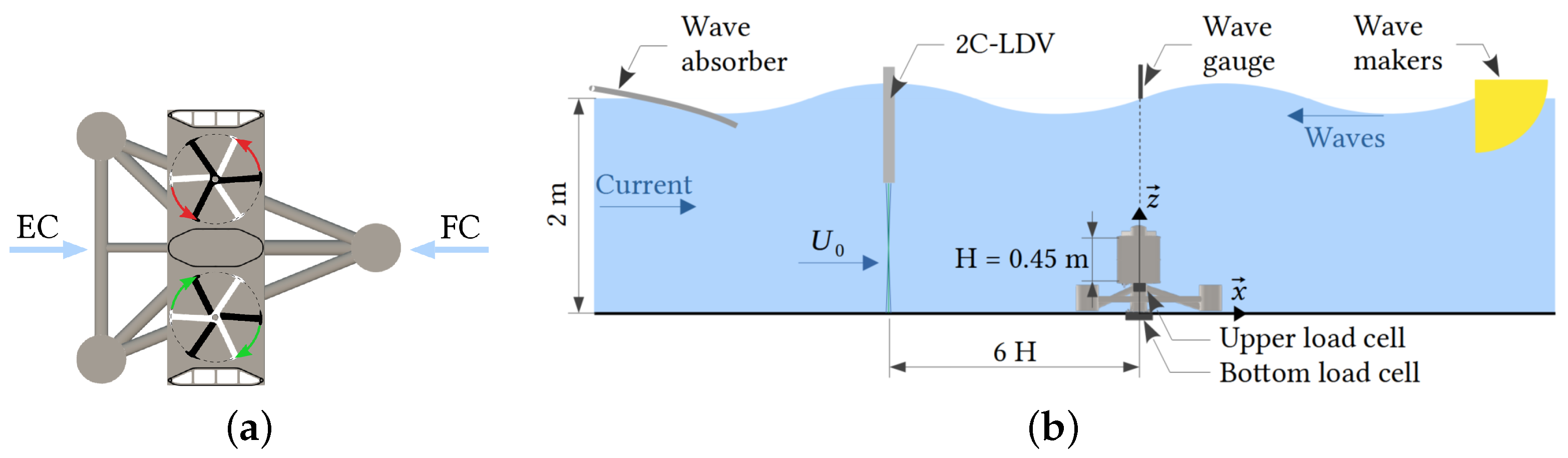
2.2. Experimental Setup

The 2-VATT model is tested in the Ifremer wave and current flume tank in Boulogne-sur-mer, France (Figure 1b), whose depth is $H_{wat}$ = 2 m and width is 4 m. It is operated at a velocity setpoint of 0.8 m.s${}^{-1}$ in its low turbulence configuration with the inlet conditioned by a honeycomb structure and a uniform grid [24]. The 2-VATT is placed in the ebb tide configuration at the centre of the tank $(x,y,z)=(0,0,0)$ with x in the main flow direction, y towards the wall and z towards the free surface with $z=0$ at the tank bottom. The 2-Component Laser Doppler Velocimeter (2C-LDV) measures the velocities $(u,v)$ along $(x,y)$ at $x=-6H$ at the centre of the turbine capture area, i.e., $(y,z)=(0,0.505)$ m. At this far upstream distance, the flow is not disturbed by the 2-VATT [23]. The time average of u at this location is considered as the reference far upstream velocity and is $U_0$ = 0.825 m.s${}^{-1}$.

In addition to the current, waves are generated to propagate against it, like during ebb tides at the Paimpol-Bréhat offshore test site [8]. To do so, wave makers are immersed downstream of the test section and a wave absorber is installed upstream [24]. In that configuration, the wave–current interaction tends to increase the wave height and shorten the wave length compared to waves on still water [25]. A servo type wave height meter (Kenek SHT3-30) measures the free surface elevation ($\eta$) right above the 2-VATT at $(x,y)=(0,0)$. Seven wave cases are presented in this study, including one irregular wave case noted $JS$ and six regular wave cases noted $f0-A-$, which indicates first the wave frequency and then the amplitude level (

Table 1. Wave against current cases’ characteristics measured in the tank without a turbine.

Case	Wave Type	${\mathit{f}}_{\mathit{\eta }}$ (Hz)	${\mathit{T}}_{\mathit{p}}$ (s)	${\mathit{A}}_{\mathit{\eta }}$ (mm)
$f00A0$	No wave	−	−	−
$f02A1$	Regular	0.2	5.0	30
$f03A1$	Regular	0.3	3.3	38
$f04A1$	Regular	0.4	2.5	37
$f04A2$	Regular	0.4	2.5	102
$f04A3$	Regular	0.4	2.5	141
$f05A1$	Regular	0.5	2.0	42
$JS$	JONSWAP	0.4	2.5	107

). The feasible wave frequency range narrows when the wave amplitude increases, and vice versa, due to the limits of the wave makers capabilities [26]. Therefore, to study the influence of the wave amplitude, we chose the frequency $f_{\eta }$ = 0.4 Hz that allows the largest amplitude range among the feasible wave conditions in the tank, and three arbitrary amplitude levels noted $A1$ (low), $A2$ (medium), and $A3$ (high). Similarly, to study the impact of the wave frequency, we chose the low amplitude level $A1$ to be able to cover a frequency range from 0.2 to 0.5 Hz. Finally, to compare the effect of regular and irregular waves on the turbine, we chose an irregular wave case with a similar peak period ($T_p=1/f_{\eta }$) and significant wave amplitude ($A_{\eta }$, the average amplitude of the highest third of the waves) to the intermediate regular wave case $f04A2$. The irregular wave case is generated according to the standard JONSWAP spectrum with a peak enhancement factor of 3.3 [27].

For all the test cases, the 2C-LDV, the wave gauge, and the turbine-related signals are acquired simultaneously over 3 min to guarantee the time convergence of the average and the standard deviation of the signals. Over this time, the 2-VATT sees between 36 and 89 wave crests when $f_{\eta }$ = 0.2 Hz and 0.5 Hz, respectively. In this setup, the blade chord based Reynolds number ($R{e}_c=c\lambda U_0/\nu$, with $\nu$ the water kinematic viscosity and $\lambda$ the tip speed ratio—Equation (5)) is of the order of $8.5\times {10}^4$, which is about 60 times smaller than at full-scale; and the Froude number based on the submergence depth ($F{r}_s=U_0/\sqrt{g(H_{wat}-H_{struc})}$ , with g = 9.81 m.s${}^{-2}$ the gravity constant) is 0.24 against 0.17 at full-scale. Due to the relatively low Reynolds number in the tank, we expect depreciated absolute rotor performance compared to the full-scale 2-VATT [28] but we expect the effect of the surface waves to be similar given the close Froude numbers.

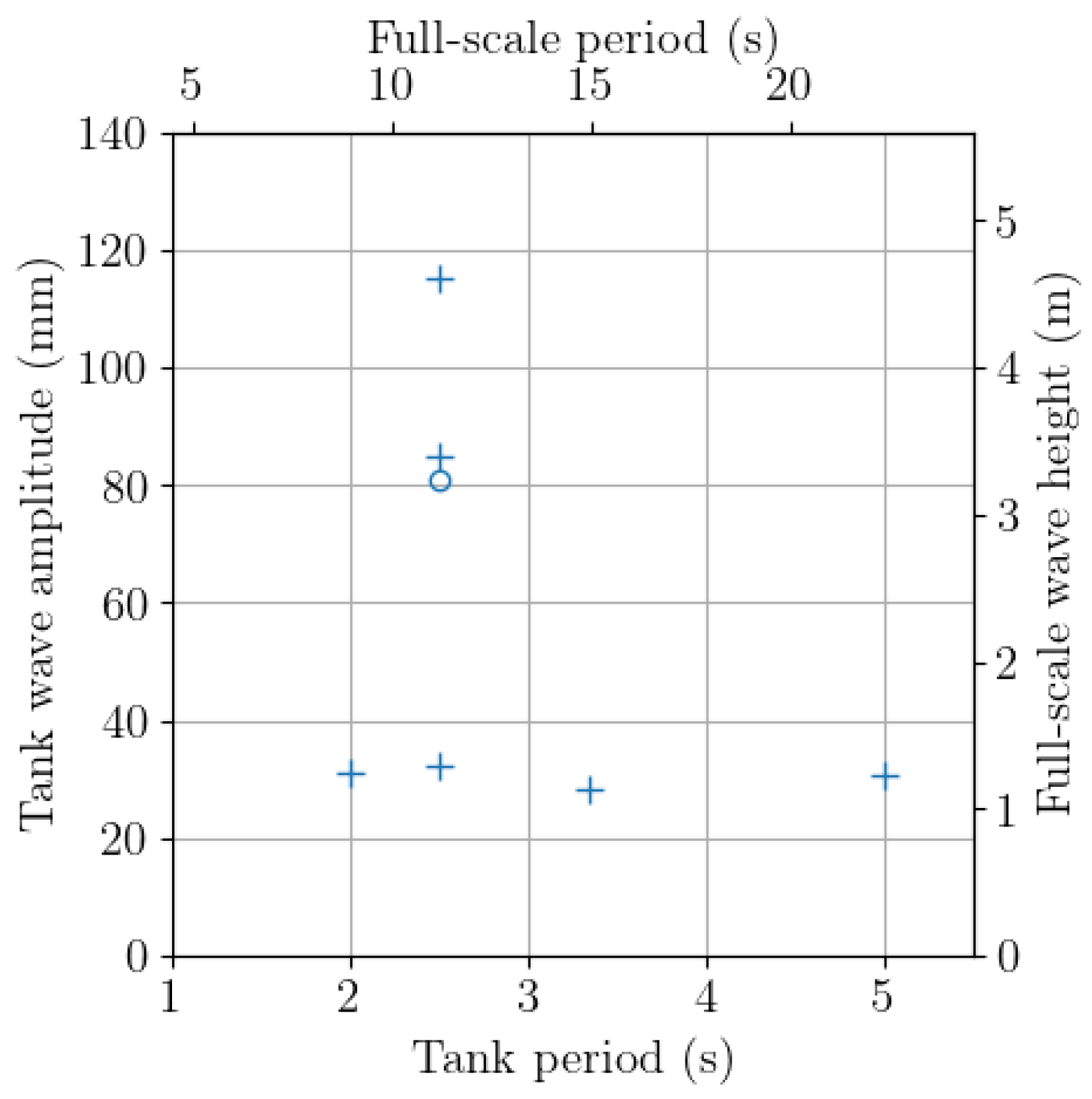
2.3. Flow Conditions

The velocity $U=u+v+w$, with $(u,v,w)$ along $(x,y,z)$, can be decomposed such that $U\left(t\right)=\overline{U}+U^{\prime }\left(t\right)$ with $U^{\prime }\left(t\right)=U^{\prime \prime }\left(t\right)+U_{\eta }\left(t\right)$, the bar above indicating the time average, the prime the overall signal fluctuating part, $U^{\prime \prime }\left(t\right)$ the turbulence contribution to the velocity fluctuation and $U_{\eta }\left(t\right)$ the waves contribution, called orbital velocity. According to the linear wave theory [29], the free surface elevation $\eta$ in the presence of regular waves propagating along x can be defined as a cosine function of the time t and the space (Equation (1) with $k_{\eta }$ the wave number and ${\omega }_{\eta }=2\pi /f_{\eta }$ the wave pulsation). This surface elevation generates orbital velocities in the propagation direction ($u_{\eta }$) and in the vertical direction ($w_{\eta }$) in the water column. The orbital velocities are defined in Equations (2) and (3) as a cosine and a sine function of time and space, respectively, with $A_u$ and $A_w$ the orbital velocity amplitudes that depend on the depth and the surface wave characteristics. When the waves propagate on top of a current, the definitions of $A_u$ and $A_w$, as well as the dispersion relation between $k_{\eta }$ and ${\omega }_{\eta }$, are modified but the orbital velocities remain defined by the same cosine and sine functions of time and space [25].

$$\eta =A_{\eta }cos(k_{\eta }x-{\omega }_{\eta }t)$$

(1)

$$u_{\eta }=A_u\left(z\right)cos(k_{\eta }x-{\omega }_{\eta }t)$$

(2)

$$w_{\eta }=A_w\left(z\right)sin(k_{\eta }x-{\omega }_{\eta }t).$$

(3)

The flow characteristics in the Ifremer’s tank in the wave opposing the current cases considered in this study were first presented in Saouli et al. [30] and thoroughly described in Magnier [26]. Figure 2 displays the wave amplitude with regard to the period measured in the tank without a turbine for the seven wave cases and shows the equivalent wave height and period at full-scale according to the Froude similitude law. At full-scale, the $A2$ (medium) wave amplitude level was roughly the limit below which the 1 MW-rated demonstrator of the ducted 2-VATT was operating and above which the rotors were parked to avoid extreme loading on the structure. At the first order for regular waves, Saouli et al. [30] obtain the orbital velocity $U_{\eta }\left(t\right)$ by filtering the velocity signal around the wave frequency. Then, the remaining velocity fluctuation is fully attributed to the turbulence $U^{\prime \prime }\left(t\right)$. Defined that way, Figure 3 presents the streamwise average velocity and turbulence intensity profiles for all the wave cases, with $\sigma$ indicating the standard deviation. The transverse average velocities $(\overline{v},\overline{w})$ are insignificant. The profiles labelled $CO$ refer to the tank configuration in current only with the wave makers and absorber out of the water whereas the $f00A0$ profiles refer to the conditions in current only with the wave makers and absorber immersed but inactive. It appears that the immersion of the wave makers and absorber in the top 0.5 m of the water column significantly modifies the average velocity and turbulence intensity profiles with a velocity increase in the bottom part of the tank and a turbulence increase in the top part. That being said, $\overline{u}$ and $\sigma \left(u^{\prime \prime }\right)/\overline{u}$ profiles remain rather homogeneous over the 2-VATT capture height, from z = 0.28 to 0.73 m. This observation justifies the use of a single velocity measurement point at the centre of the capture area as the reference velocity $U_0$. In the following, the $f00A0$ current only case will be the reference when assessing the effect of surface waves. Furthermore, Figure 4 displays the oscillation amplitude of the streamwise and vertical orbital velocities for all the regular wave cases, presented in Magnier [26]. For the low amplitude cases ($A1$), both the streamwise and vertical orbital velocities are less than 0.05 m.s${}^{-1}$ (0.06 $U_0$) over the whole 2-VATT height. As predicted by the linear wave theory, the orbital velocity amplitude increases with the wave amplitude such that $A_u\simeq 0.09U_0$ in $f04A2$ and $A_u\simeq 0.13U_0$ in $f04A3$ at the turbine mid-height.

Among the seven wave cases, we will especially focus on the regular wave case $f04A2$ and the irregular wave case compared to the current only case. Using the linear wave theory, Figure 5 displays one theoretical period of the surface elevation in $f04A2$ along with the streamwise and vertical velocities at the turbine mid-height ($z=0.505$ m), where the velocity characteristics are approximately $\overline{u}=U_0=0.825$ m.s${}^{-1}$, $A_u=0.09U_0$ and $A_w=0.04U_0$ (Figure 4). The figure also displays the angle ${\alpha }_w$ between the total velocity direction and the horizontal direction. Figure 5 shows that the streamwise velocity fluctuation is in phase opposition with regard to the surface elevation while the vertical orbital velocity is $\pi /2$ out of phase. In wave–current conditions, the total velocity direction is in phase with w and reaches almost ±2${}^{\circ }$ with regard to the horizontal direction. In addition, Figure 6a presents the Probability Density Function (PDF) of the streamwise velocity measured with the 2C-LDV upstream of the 2-VATT at $x=-6H$ and at the centre of the projected capture area in these three flow conditions. The arithmetic average of the velocity at this position is equal to $U_0$ in the three cases but the velocity distribution around that average value varies. In the presence of waves, the velocity range is extended compared to the current only case, due to the orbital velocities induced by the waves. However, with regular waves, the distribution presents two maxima, related to the periodical increase and decrease of the velocity occurring when a wave through and crest passes, respectively; whereas a single PDF maxima is present at the average value in $JS$ as the orbital velocities do not have favourite amplitudes with irregular waves. Additionally, Figure 6b presents the power spectral density of the same 2C-LDV streamwise velocity measurements. The power spectral densities of the fluctuating part of u ($\mathcal{S}(u^{\prime }/U_0)$) are computed using Welch’s method with 64 s long windows and a 50% overlap. The spectral analysis reveals a strong energy peak at the wave frequency, as expected, with a sharp peak for the regular wave case and an increased level of energy between about 0.25 and 0.55 Hz in the JONSWAP case.

2.4. Data Processing

The power coefficient of each rotor column $C_{Pcol}$ is computed as in Equation (4) with $P_{col}\left(t\right)=Q\left(t\right)\omega \left(t\right)$ and t the time. The reference surface is that of the rotors projected area ($2D{H}_{blade}$) and the torque signal considered is corrected by the friction torque induced by the seals and the transmission system for each rotor column [23]. Then, the overall average power coefficient $\overline{C_P}$ is the average of the two $C_{Pcol}\left(t\right)$ and the power fluctuation is analysed considering the average standard deviation between the two rotor columns, denoted as $\overline{\sigma }\left(C_{Pcol}\right)$.

$$C_{Pcol}\left(t\right)=\frac{P_{col}\left(t\right)}{\rho D{H}_{blade}{U}_0^3}.$$

(4)

The tip speed ratio ($\lambda$) is defined in Equation (5). Thus, ${\lambda }_0$ refers to the tests with parked rotors and ${\lambda }_{opt}$ refers to the those at the operating point providing the maximal power coefficient. The force and moment coefficients are defined in Equations (6) and (7) for the components along x with the four rotors’ projected area as a reference surface. They are defined the same way for the loads along y and z. The loads measured without current at ${\lambda }_0$ are subtracted to consider only the hydrodynamic loads on the device without the gravity. In this study, we consider the forces applied by the turbine on the gravity base—measured by the upper load cell—and the moments applied to the ground, measured by the bottom load cell (Figure 1b). These are the loads to consider for the design of a stable gravity base. For all the hydrodynamic coefficients the reference upstream velocity measurement $U_0$ is averaged with the appropriate power weighting (power 1 for $\lambda$, 2 for the load coefficients, and 3 for the power).

$$\lambda \left(t\right)=\frac{\omega \left(t\right)R}{U_0}$$

(5)

$$C_x\left(t\right)=\frac{F_x\left(t\right)}{2\rho D{H}_{blade}{U}_0^2}$$

(6)

$$C_{Mx}\left(t\right)=\frac{M_x\left(t\right)}{2\rho RD{H}_{blade}{U}_0^2}.$$

(7)

In addition to the load coefficients evolution with the tip speed ratio, we also analyse their probability density functions with 50 equal-width bins to consider the load distributions and extrema. The extreme load value is considered as the maximum between the absolute value of the first and the last percentile (max[abs(p01), abs(p99)]) and the load range is considered as the difference between p01 and p99. The correlation between the wave-induced velocity fluctuation and the loads fluctuation is analysed by computing the normalised cross-correlation coefficient $\mathcal{R}$ with regard to the time lag ($\tau$) between the free surface elevation ($\eta$) above the 2-VATT and the loads or the rotor torque (Equation (8), with s indicating the loads or torque signal).

$$\mathcal{R}\left({\eta }^{\prime },s^{\prime }\right)\left[\tau \right]=\frac{\overline{\left(\eta \left(t\right)-\overline{\eta }\right)\left(s(t+\tau )-\overline{s}\right)}}{\sqrt{\overline{{\left(\eta \left(t\right)-\overline{\eta }\right)}^2}\overline{{\left(s\left(t\right)-\overline{s}\right)}^2}}}.$$

(8)

We also study the fluctuation of the rotor torque, the drag and lift coefficients averaged according to the wave phase with 3 degrees phase bins, indicated by a tilde above the symbols. The wave phase is obtained by Hilbert transform of the surface elevation signal filtered at the wave frequency ± 0.1 Hz. Finally, the Fourier transforms ($\mathcal{F}$) of $Q^{\prime }$, $F_x^{\prime }$, and $F_z^{\prime }$ are computed as well as their coherence function with the upstream velocity measurement using Welch’s method with 32 s long windows and 50% overlap to analyse the periodical characteristics of the 2-VATT related signals compared to those of the wave-induced flow fluctuation.

3. Effect of Surface Waves Opposing the Current on the 2-VATT Behaviour

3.1. Wave Amplitude and Frequency Effect

Figure 7 gives an overview of the wave effect on the average and standard deviation of the power performance and on the loads of the ducted 2-VATT with regard to the tip speed ratio. The general trend is that the presence of surface waves barely affects the average values at the optimal operating point but it increases the standard deviations, whether the 2-VATT rotors are parked or in operation. In addition, the waves modify the evolution of the power coefficient with the tip speed ratio, both on average and in fluctuation, but they do not affect the one of the load coefficients. More specifically, we observe an average power coefficient decrease with the wave amplitude at the tip speed ratios below ${\lambda }_{opt}$, without changing the maximal $\overline{C_P}$ at $\overline{\lambda }=1.6$. The data may indicate an increase of ${\lambda }_{opt}$ with $A_{\eta }$, but complementary measurements at $\overline{\lambda }>1.6$ would be needed to confirm this supposition. In addition, the waves induce a slight increase of the average loads on the 2-VATT with less than 5% difference compared to the case without waves, and without modifying the loads evolution with regard to $\lambda$. The limited effect of the surface waves on the average power and loads is consistent with the homogeneity of the average velocity profiles over the wave cases (Figure 3a). The power performance decrease at the low tip speed ratios may reveal an increase of the dynamic stall due to the wave-induced velocity fluctuation (Figure 4).

Additionally, those wave-induced orbital velocities strongly affect the standard deviation of the power and loads coefficients. Indeed, the latter increase linearly with the wave amplitude such that an $A_{\eta }$ increase of 0.1 m generates roughly a 2, 3, and 4 times higher $\sigma \left(C_{Pcol}\right)$, $\sigma \left(C_z\right)$ and $\sigma \left(C_x\right)$, respectively, at ${\lambda }_{opt}$ (Figure 8). As a consequence, $\sigma \left(C_z\right)\simeq \overline{C_z}$ for the wave case with the highest amplitude. Those linear trends between the load standard deviations and the wave amplitude are rather independent of $\lambda$, which indicates a low interaction between the rotors rotation and the waves on the loadings. We only observe an offset in $\sigma \left(C_x\right)$ and $\sigma \left(C_{My}\right)$ when comparing between ${\lambda }_0$ and ${\lambda }_{opt}$ due to the blades passing, but the linear trends with $A_{\eta }$ are unchanged (Figure 8). Regarding the power coefficient, the waves impact on $\overline{\sigma }\left(C_{Pcol}\right)$ grows with $\lambda$. Indeed, the slope of the linear fit with $A_{\eta }$ increases with $\lambda$, which indicates an interaction between the rotors rotation and the waves on the power performance, unlike the loads. To the authors’ knowledge, such a linear relationship between the surface wave height and the load’s standard deviation of a turbine has never been shown before. However, using a theoretical model, Xin et al. [31] also found a linear relationship between the wave height and the standard deviation of the horizontal force applied to a bottom-fixed vertical slender cylinder subjected to surface waves and a tidal current.

In the design process, under the assumption of a normal law of distribution, the expected extreme loads on the turbine can be estimated by combining the average and the standard deviation values. For instance, the extreme drag coefficient value is estimated as $C_{x,max}=\overline{C_x}+3\sigma \left(C_x\right)$. Here, $C_{x,max}=3.01$ at the optimal operating point in the medium wave case $f04A2$ against 1.32 with the rotors parked in the extreme wave case $f04A3$. This result justifies the choice to park the rotors in the presence of extreme wave conditions to limit structural damages. Following the linear trends in Figure 8 for regular waves at 0.4 Hz, we find that the extreme loads on the turbine would be greater with the rotors parked compared to the limit case at ${\lambda }_{opt}$ with intermediate wave conditions ($f04A2$) if $A_{\eta }>0.18$ m, which gives a 7.2 m wave height at full-scale according to the Froude similitude law. That wave height at sea is likely to be encountered during winter storms, with about a 5-year return period at the Paimpol-Bréhat tidal turbine test site [32].

Still looking at Figure 7, it appears that regular and irregular waves with similar peak periods and significant wave amplitudes, namely $f04A2$ and $JS$ (Table 1), affect the $C_P$ evolution with $\lambda$ the same way, both in terms of average and fluctuation. However, we observe few load differences between the regular and the irregular wave cases. The average loads in $JS$ at ${\lambda }_0$ are equal to the case without waves while they are slightly higher with regular waves. In addition, with the rotors in operation, $\overline{C_z}$ is similar with both regular and irregular waves but $\overline{C_x}$ and $\overline{C_{My}}$ are a few percent lower in $JS$; while $\sigma \left(C_x\right)$ and $\sigma \left(C_{My}\right)$ are unchanged, but $\sigma \left(C_z\right)$ is 37% lower in $JS$ compared to $f04A2$.

Beyond the wave amplitude, its frequency is also expected to affect the 2-VATT response. However, the power and drag coefficients evolution with the tip speed ratio are almost the same in the four wave cases at variable frequency (Figure 9). Due to the wave–current interaction and the wave maker amplitude limits at low frequencies, the multiple wave frequency cases could only be generated at the amplitude level $A1$. The previous results on the wave amplitude effect showed that the 2-VATT response is barely affected by waves of that amplitude level. Hence, we assume that the absence of a frequency effect observed here is actually due to the smallness of the waves amplitude. Indeed, the wave-induced velocity fluctuation in those wave cases is less than 6% of the average velocity at the turbine mid-height (Figure 4).

3.2. Wave–Current–Turbine Interaction

To better understand how the surface waves increase the ducted 2-VATT power and loads fluctuation, we focus on the $f04A2$ regular wave case and the $JS$ irregular wave case. The turbine response is first studied with parked rotors (at ${\lambda }_0$) to look at the wave’s effects on the static structure before addressing the interaction with the turbine in operation (at ${\lambda }_{opt}$).

3.2.1. Parked Turbine

The waves’ direction is collinear with the current direction, which causes additional velocity fluctuation in the streamwise and the vertical direction (Figure 4). Therefore, the ranges of $C_x$, $C_z$ and $C_{My}$ between the first and the last percentile (p99–p01) are strongly extended in the presence of surface waves (Figure 10). Indeed, the three load ranges are 5.7 to 6.7 times higher in $f04A2$ at ${\lambda }_0$ than without waves (

Table 2. Load range (p99–p01) and extreme value (max[abs(p01), abs(p99)]) ratios between the cases with waves and the case $f00A0$ without waves at ${\lambda }_0$.

(a). Ratio of Load Ranges
Case	$C_x$	$C_z$	$C_{My}$
$f04A2/f00A0$	6.68	5.72	6.22
$JS/f00A0$	9.58	5.87	8.81
(b). Ratio of Extreme Loads
Case	$C_x$	$C_z$	$C_{My}$
$f04A2/f00A0$	1.41	1.87	1.38
$JS/f00A0$	1.76	1.96	1.49

). That range increase goes along with extreme values breaking by +41% for $C_x$ and $C_{My}$ and by +87% for $C_z$ in $f04A2$ compared to $f00A0$. Those results are critical for the structural design both in terms of fatigue and ultimate limit. On the other hand, the waves collinear with the current barely modify the transverse velocity v, so the three other load components are less affected by the presence of those surface waves. Furthermore, we notice that the $C_x$ and $C_{My}$ ranges are more than 40% higher in irregular waves than in regular ones, although Figure 7 reveals higher standard deviations with the regular wave case. That result is due to the load distribution difference between the regular wave case, with two PDF modes, and the irregular wave case, with a single PDF mode. The difference of load distribution mimics the difference of velocity distribution between the two cases (Figure 6), which indicates a strong correlation between the wave-induced velocity fluctuation and the load fluctuation.

Figure 11a presents the cross-correlation coefficients ($\mathcal{R}$) of the surface elevation measurement above the 2-VATT with a rotor column torque and with the whole 2-VATT drag and lift forces in the $f04A2$ case. The cross-correlation coefficient extrema are almost ±1 for $F_x$ and $F_z$, and $\mathcal{R}$ is close to ±0.8 for the torque, which already quantifies the strong impact of the surface waves on the loads and rotor torque fluctuation. The interpretation of the time lags at which $\mathcal{R}$ is maximum or minimum is not straightforward however, and requires us to return to the linear wave theory. As presented in Section 2.3, in this wave-against-current case, the streamwise orbital velocity ($u_{\eta }$) is in phase opposition with the surface elevation while the vertical one ($w_{\eta }$) (and so the pitch angle between the velocity and the turbine) is $\pi /2$ out of phase (Figure 5), i.e., a quarter of the wave period ($Tp$/4 = 0.625 s in $f04A2$). Assuming that the fluctuations of the rotor torque Q and of $F_x$ are mainly caused by the fluctuation of u and that the ones of $F_z$ can be mainly attributed to the fluctuation of w, we expect $F_x$ and Q to be in phase with $u_{\eta }$ (and so in phase opposition with $\eta$) while $F_z$ would be in phase with $w_{\eta }$ (and so $\pi /2$ out of phase with $\eta$). That assumption is valid for Q as a minimum of $\mathcal{R}(\eta ,Q)$ occurs with zero time lag, meaning that a crest of $\eta$ generates a trough of Q without lag, similarly to $u_{\eta }$. The two maxima at $Tp/2=\pm$1.25 s reveal the maxima of Q generated by the surface elevation trough. That perfect phase opposition between $\eta$ and Q is also observed in the wave phase-averaged graphs (Figure 11b). In contrast, the minimum of $\mathcal{R}(\eta ,F_x)$ expected with a 0 s lag, and the maximum of $\mathcal{R}(\eta ,F_z)$ expected with a $Tp$/4 = 0.625 s lag, appear with a ∼0.35 s lag compared to the expected values. That lag is also observed in Figure 11b as the wave phase averages of the fluctuating $C_x$ and $C_z$ are ∼$-\pi /4$ = −45${}^{\circ }$ shifted compared to the relative phase of u and w with regard to $\eta$ (Figure 5). Phase shifts from −5 to −80${}^{\circ }$ between the surface elevation and the drag force were also observed by Martinez et al. [14] on a HATT. Those results mean that the force extrema (crest or through) occur before the surface elevation extrema and so before the orbital velocity extrema, as it was demonstrated regarding the force exerted by surface waves on piles by Morison et al. [15]. According to the latter, the phase shift increases with the pile diameter relative to the water depth. Therefore, the small blade size relative to the water depth, by opposition to the large size of the whole 2-VATT, may explain the absence of such a phase shift on the rotor torque Q while it is observed on the whole turbine loads.

3.2.2. Operating Turbine

To look at the combination of the wave-induced loads with the rotors rotation-induced loads, Figure 12 presents the loads’ PDF with the turbine operating at ${\lambda }_{opt}$ and ${\lambda }_0$ when subjected to the regular wave case $f04A2$. The results show that $C_z$ is unaffected by the rotors rotation as its distribution is the same whether with parked or operating rotors. $C_x$ and $C_{My}$ appear to be shifted on average due to rotors thrust and their distributions are slightly widened but they remain with two modes at ${\lambda }_{opt}$ like at ${\lambda }_0$. However, the distribution of $C_y$ and $C_{Mx}$ shows two modes at ${\lambda }_{opt}$, whereas these were made of a single mode at ${\lambda }_0$. $C_y$ and $C_{Mx}$ bimodal distribution was already observed without waves and was supposed to be due to the asymmetrical thrust of the two rotor columns when their angular position is asymmetrical [33]. Therefore, the loads’ PDF at ${\lambda }_{opt}$ presents a combination of the wave-induced signature (on $C_x$ and $C_{My}$) and of the rotor-induced one (on $C_y$ and $C_{Mx}$) without showing a clear interaction between the two. Similarly, the cross-correlations of the surface elevation with a rotor column torque and with the turbine drag and lift forces are barely affected by the rotor’s operation. We only observe a reduction of $\mathcal{R}(\eta ,Q)$ extrema to less than ±0.7 with a slight time lag that could indicate the appearance of some added mass effects on the rotating rotors.

The Fourier transform ($\mathcal{F}$) of one rotor column torque in the case without waves $f00A0$, with regular waves $f04A2$, and with irregular waves $JS$ gives a better insight into the origin of the increased load fluctuation in presence of surface waves and into the wave–rotation interaction (Figure 13). First, without waves, the torque spectral content is mainly located at three and six times the rotational frequency ($f_{\omega }$), which corresponds to the blade passing frequency since the rotor columns are made of two levels of out-of-phase three-bladed rotors. When adding surface waves to the current, those rotor-induced spectral peaks are unchanged but other peaks raise. A strong peak appears at the wave frequency ($f_{\eta }$) both with regular and irregular waves on the Fourier transform of the torque and of the loads, similar to the results on HATTs [11,12,16]. The $\mathcal{F}\left(C_Q\right)$ peak at $f_{\eta }$ dominates the rotor-induced peaks in regular waves whereas the peaks at 3 and 6$f_{\omega }$ remain the highest with irregular waves. Both in the regular and irregular wave cases, the coherence function between the upstream velocity measurement and the torque, the drag and the lift force reaches almost 1 around $f_{\eta }$, meaning that the torque and loads spectral content at that frequency is fully due to the wave-induced orbital velocity (Figure 14). Those coherence functions also reveal that the 2-VATT responds to the whole wave spectrum width in the irregular wave case as the three coherence functions exceed 0.5 from 0.25 to 0.55 Hz. Finally, in addition to the strong peak at $f_{\eta }$ in the torque Fourier transform, additional peaks appear at $6f_{\omega }\pm k{f}_{\eta }$, with k = 1 and 2, both with regular and irregular waves. Those peaks evidence the interaction between the periodic loadings induced by the surface waves and those induced by the rotor columns rotation. Similar peaks combining the turbine rotational frequency harmonics and the wave frequency have also been observed in horizontal axis tidal turbines by Draycott et al. [16]. These are explained by a rotational sampling of the waves by the turbine blades that make several rotations during one wave period.

4. Conclusions

While numerous studies have analysed the effect of surface waves on horizontal axis tidal turbines, only a few have considered vertical axis ones in limited wave and operating conditions, and none have considered twin vertical axis tidal turbines (2-VATT). In this paper, we tested a 1/20 scale bottom mounted and ducted 2-VATT, similar to HydroQuest’s 1 MW-rated demonstrator, in a larger range of wave and operating conditions compared to the previous studies on vertical axis turbines. Seven wave conditions are presented to independently assess the effect of the waves’ amplitudes and their frequencies, as well as to compare the effect of regular and irregular waves on the turbine behaviour.

The results show that the maximal average power coefficient is unaffected by the presence of waves, although the power curve may be slightly shifted towards higher tip speed ratios. The average hydrodynamic loads on the turbine increase with the regular wave amplitude but they remain less than 5% higher than without waves. The effect of the waves on the power and loads fluctuation is much more important. The standard deviation of the power, the drag, and the lift follow a linear trend with a slope of 2, 3, and 4, respectively, with regard to the wave amplitude. However, the too-low wave amplitude of the variable-frequency cases prevented us from highlighting the wave frequency’s influence on the turbine behaviour. Looking in more detail at the effect of the intermediate frequency and amplitude wave case, we find that the drag, lift, and pitching moment distribution ranges are extended to up to 6.7 times greater, and that the extreme values are exceeded by 40 to 90% with the regular waves compared to the conditions with current only. The rotor torque and load fluctuation increase is highly correlated with the surface elevation and the orbital velocity, with a cross-correlation coefficient exceeding 0.75 and a coherence function exceeding 0.5 on all the wave spectrum bandwidth.

In addition, the 2-VATT response is similar in terms of average and standard deviation of the power and the loads between the regular and irregular wave cases of similar period and height. However, the streamwise load range is 1.4 times larger in irregular waves and the extreme values are exceeded compared to the regular wave case due to the load distribution shape difference, with a single mode in irregular waves and two in regular ones. Thus, testing vertical axis tidal turbine models in regular waves only is insufficient to accurately predict the wave-induced loads for the mechanical design of full-scale turbines operating at sea.

In the future, tests with several wave directions relative to the current direction could extend the present study and improve the understanding of the ducted 2-VATT response to surface waves at sea. Furthermore, studying the effect of the surface waves on the turbine wake would also be of interest from the perspective of tidal turbine farm deployments.

References

1. IEA-OES. Tidal Current Energy: Developments Highlights; Technical Report; International Energy Agency: Paris, France, 2023. [Google Scholar]
2. Sentchev, A.; Nguyen, T.D.; Furgerot, L.; Bailly du Bois, P. Underway velocity measurements in the Alderney Race: Towards a three-dimensional representation of tidal motions. Philos. Trans. R. Soc. A 2020, 378, 20190491. [Google Scholar] [CrossRef] [PubMed]
3. Cossu, R.; Penesis, I.; Nader, J.R.; Marsh, P.; Perez, L.; Couzi, C.; Grinham, A.; Osman, P. Tidal energy site characterisation in a large tidal channel in Banks Strait, Tasmania, Australia. Renew. Energy 2021, 177, 859–870. [Google Scholar] [CrossRef]
4. Mercier, P.; Guillou, S. The impact of the seabed morphology on turbulence generation in a strong tidal stream. Phys. Fluids 2021, 33, 055125. [Google Scholar] [CrossRef]
5. Guillou, N.; Chapalain, G.; Neill, S.P. The influence of waves on the tidal kinetic energy resource at a tidal stream energy site. Appl. Energy 2016, 180, 402–415. [Google Scholar] [CrossRef]
6. Bennis, A.C.; Furgerot, L.; Bailly Du Bois, P.; Poizot, E.; Méar, Y.; Dumas, F. A winter storm in Alderney Race: Impacts of 3D wave–current interactions on the hydrodynamic and tidal stream energy. Appl. Ocean Res. 2022, 120, 103009. [Google Scholar] [CrossRef]
7. Perez, L.; Cossu, R.; Grinham, A.; Penesis, I. Tidal turbine performance and loads for various hub heights and wave conditions using high-frequency field measurements and Blade Element Momentum theory. Renew. Energy 2022, 200, 1548–1560. [Google Scholar] [CrossRef]
8. Moreau, M.; Germain, G.; Maurice, G.; Richard, A. Sea states influence on the behaviour of a bottom mounted full-scale twin vertical axis tidal turbine. Ocean Eng. 2022, 265, 112582. [Google Scholar] [CrossRef]
9. Gaurier, B.; Ordonez-Sanchez, S.; Facq, J.V.; Germain, G.; Johnstone, C.; Martinez, R.; Salvatore, F.; Santic, I.; Davey, T.; Old, C.; et al. MaRINET2 Tidal Energy Round Robin Tests—Performance Comparison of a Horizontal Axis Turbine Subjected to Combined Wave and Current Conditions. J. Mar. Sci. Eng. 2020, 8, 463. [Google Scholar] [CrossRef]
10. Barltrop, N.; Varyani, K.S.; Grant, A.; Clelland, D.; Pham, X. Wave-current interactions in marine current turbines. Proc. Proc. Inst. Mech. Eng. Part M J. Eng. Marit. Environ. 2006, 220, 195–203. [Google Scholar] [CrossRef]
11. Gaurier, B.; Davies, P.; Deuff, A.; Germain, G. Flume tank characterization of marine current turbine blade behaviour under current and wave loading. Renew. Energy 2013, 59, 1–12. [Google Scholar] [CrossRef]
12. Martinez, R.; Payne, G.S.; Bruce, T. The effects of oblique waves and currents on the loadings and performance of tidal turbines. Ocean Eng. 2018, 164, 55–64. [Google Scholar] [CrossRef]
13. Ordonez-Sanchez, S.; Allmark, M.; Porter, K.; Ellis, R.; Lloyd, C.; Santic, I.; O’Doherty, T.; Johnstone, C. Analysis of a Horizontal-Axis Tidal Turbine Performance in the Presence of Regular and Irregular Waves Using Two Control Strategies. Energies 2019, 12, 367. [Google Scholar] [CrossRef]
14. Martinez, R.; Ordonez-Sanchez, S.; Allmark, M.; Lloyd, C.; O’Doherty, T.; Germain, G.; Gaurier, B.; Johnstone, C. Analysis of the effects of control strategies and wave climates on the loading and performance of a laboratory scale horizontal axis tidal turbine. Ocean Eng. 2020, 212, 107713. [Google Scholar] [CrossRef]
15. Morison, J.; Johnson, J.; Schaaf, S. The Force Exerted by Surface Waves on Piles. J. Pet. Technol. 1950, 2, 149–154. [Google Scholar] [CrossRef]
16. Draycott, S.; Steynor, J.; Nambiar, A.; Sellar, B.; Venugopal, V. Rotational sampling of waves by tidal turbine blades. Renew. Energy 2020, 162, 2197–2209. [Google Scholar] [CrossRef]
17. Ouro, P.; Dené, P.; Garcia-Novo, P.; Stallard, T.; Kyozuda, Y.; Stansby, P. Power density capacity of tidal stream turbine arrays with horizontal and vertical axis turbines. J. Ocean Eng. Mar. Energy 2022, 9, 203–208. [Google Scholar] [CrossRef]
18. Bachant, P.; Wosnik, M. Experimental Investigation of Helical Cross-Flow Axis Hydrokinetic Turbines, Including Effects of Waves and Turbulence. In Proceedings of the ASME-JSME-KSME 2011 Joint Fluids Engineering Conference, Shizuoka, Japan, 24–29 January 2011; pp. 1895–1906. [Google Scholar] [CrossRef]
19. Zhang, X.w.; Zhang, L.; Wang, F.; Zhao, D.Y.; Pang, C.Y. Research on the unsteady hydrodynamic characteristics of vertical axis tidal turbine. China Ocean Eng. 2014, 28, 95–103. [Google Scholar] [CrossRef]
20. Lust, E.E.; Bailin, B.H.; Flack, K.A. Performance characteristics of a cross-flow hydrokinetic turbine in current only and current and wave conditions. Ocean Eng. 2021, 219, 108362. [Google Scholar] [CrossRef]
21. Vergaerde, A.; De Troyer, T.; Muggiasca, S.; Bayati, I.; Belloli, M.; Kluczewska-Bordier, J.; Parneix, N.; Silvert, F.; Runacres, M.C. Experimental characterisation of the wake behind paired vertical-axis wind turbines. J. Wind. Eng. Ind. Aerodyn. 2020, 206, 104353. [Google Scholar] [CrossRef]
22. Müller, S.; Muhawenimana, V.; Wilson, C.A.; Ouro, P. Experimental investigation of the wake characteristics behind twin vertical axis turbines. Energy Convers. Manag. 2021, 247, 114768. [Google Scholar] [CrossRef]
23. Moreau, M.; Germain, G.; Maurice, G. Experimental performance and wake study of a ducted twin vertical axis turbine in ebb and flood tide currents at a 1/20th scale. Renew. Energy 2023, 214, 318–333. [Google Scholar] [CrossRef]
24. Gaurier, B.; Germain, G.; Facq, J.V.; Bacchetti, T. Wave and Current Flume Tank of IFREMER at Boulogne-sur-mer. Description of the Facility and Its Equipment; Technical Report; IFREMER: Plouzané, France, 2018. [Google Scholar] [CrossRef]
25. Brevik, I.; Bjørn, A. Flume experiment on waves and currents. I. Rippled bed. Coast. Eng. 1979, 3, 149–177. [Google Scholar] [CrossRef]
26. Magnier, M. Étude Expérimentale des Courants de Marée et de la Houle sur la Dynamique Tourbillonnaire d’une Variation Bathymétrique et sur le Comportement d’une Hydrolienne. Ph.D. Thesis, Université de Lille, Lille, France, 2023. [Google Scholar]
27. Hasselmann, K.; Barnett, T.P.; Bouws, E.; Carlson, H.; Cartwright, D.E.; Eake, K.; Euring, J.A.; Gicnapp, A.; Hasselmann, D.E.; Kruseman, P.; et al. Measurements of wind-wave growth and swell decay during the joint North Sea wave project (JONSWAP). Erganzungsheft zur Deutschen Hydrographischen Zeitschrift. 1973. A(8), Nr 12. Available online: https://pure.mpg.de/pubman/faces/ViewItemOverviewPage.jsp?itemId=item_3262854 (accessed on 1 January 2020).
28. Bachant, P.; Wosnik, M. Effects of Reynolds Number on the Energy Conversion and Near-Wake Dynamics of a High Solidity Vertical-Axis Cross-Flow Turbine. Energies 2016, 9, 73. [Google Scholar] [CrossRef]
29. Molin, B. Hydrodynamique des Structures Offshore; Editions Technip: Paris, France, 2002. [Google Scholar]
30. Saouli, Y.; Magnier, M.; Germain, G.; Gaurier, B.; Druault, P. Experimental characterisation of the waves propagating against current effects on the wake of a wide bathymetric obstacle. In Proceedings of the 18ème Journées de l’Hydrodynamique, Poitiers, France, 22–24 November 2022; pp. 1–12. [Google Scholar]
31. Xin, Z.; Li, X.; Li, Y. Coupled effects of wave and depth-dependent current interaction on loads on a bottom-fixed vertical slender cylinder. Coast. Eng. 2023, 183, 104304. [Google Scholar] [CrossRef]
32. EDF; SEENEOH. Paimpol-Bréhat Tidal Turbine Test Site Documentation v1.2; Technical Report; EDF: London, UK, 2022. [Google Scholar]
33. Moreau, M.; Bloch, N.; Maurice, G.; Germain, G. Experimental study of the upstream bathymetry effects on a ducted twin vertical axis tidal turbine. Renew. Energy 2023. under review. [Google Scholar] [CrossRef]
Figure 1. (a) Schematic top view of the turbine operating in Ebb tide or Flood tide Configuration (EC or FC, respectively). (b) Schematic side view of the experimental setup in Ifremer’s tank with waves opposing the current direction.
Jmse 11 01895 g001
Figure 2. Amplitude A η and period T p of the waves generated in the tank (left and bottom axes). The crosses represent the regular wave cases and the circle is the JONSWAP case. The right and top axes provide the waves period and height at a 20/1 scale according to Froude similitude law.
Jmse 11 01895 g002
Figure 3. Average (a) and turbulence intensity (b) streamwise velocity profiles in the classical current only case (CO), with the damping beach and wave makers immersed ( f 00 A 0 ) and in all the wave cases considered. The data are from Saouli et al. [30]. The grey area represents the 2-VATT capture height.
Jmse 11 01895 g003
Figure 4. Amplitude of the streamwise (a) and vertical (b) orbital velocities along the water depth in the regular wave cases. The data is from Magnier [26]. The grey area represents the 2-VATT capture height.
Jmse 11 01895 g004
Figure 5. Theoretical period of the surface elevation η , the streamwise and the vertical velocities u and w and the angle α w between the velocity direction and the horizontal direction, with u ¯ = 0.825 m.s 1 , A u = 0.09 u ¯ , and A w = 0.04 u ¯ . This corresponds approximately to the flow conditions in f 04 A 2 at z = 0.5 m according to the linear wave theory.
Jmse 11 01895 g005
Figure 6. (a) Probability Density Function and (b) Power spectral density of the streamwise velocity measured with the 2C-LDV at x = 6 H upstream of the 2-VATT at the centre of the projected capture area.
Jmse 11 01895 g006
Figure 7. Evolution with the tip speed ratio of the power (a), drag (b), lift (c), and pitch (d) coefficients with the average at the top and standard deviation at the bottom of each sub-figure. The C P values are normalised by the maximal average value in the f 00 A 0 case (without waves).
Jmse 11 01895 g007
Figure 8. Coefficients’ standard deviation with regard to the waves amplitude for f η = 0.4 Hz, when the turbine is parked or operating at λ o p t . Dashed lines are linear fits of the data points. The points labelled C P are the values of σ ¯ ( C P c o l ) / C P ¯ m a x .
Jmse 11 01895 g008
Figure 9. Power (a) and drag (b) coefficients with the average at the top and standard deviation at the bottom of each sub-figure. The C P are normalised by the maximal average value in the f 00 A 0 case (without waves).
Jmse 11 01895 g009
Figure 10. Probability Density Functions of the load coefficients at λ 0 computed without waves, with regular waves and with irregular waves of the same characteristic amplitude and frequency.
Jmse 11 01895 g010
Figure 11. In the case f 04 A 2 with the rotors parked, (a) the cross-correlations of the surface elevation with the torque of a rotor column, the drag and the lift forces on the turbine, and (b) the surface elevation, the torque coefficient of a rotor column, the drag and the lift coefficients averaged according to the surface elevation phase.
Jmse 11 01895 g011
Figure 12. Probability Density Functions of the load coefficients in f 04 A 2 when the 2-VATT rotors are parked (blue) against when they operate at λ o p t (orange).
Jmse 11 01895 g012
Figure 13. Fourier transform of the torque coefficient of one rotor column without waves (top), with regular waves f 04 A 2 (middle) and with irregular waves J S (bottom).
Jmse 11 01895 g013
Figure 14. Coherence function of the torque coefficient of one rotor column, the drag and lift coefficients of the 2-VATT at λ o p t with the upstream streamwise velocity measurement at x = 6 H in regular waves f 04 A 2 (top) and irregular waves J S  (bottom).
Jmse 11 01895 g014