Path Planning Method for Underwater Gravity-Aided Inertial Navigation Based on PCRB

Abstract

Gravity-aided inertial navigation system (GAINS) is an important development in autonomous underwater vehicle (AUV) navigation. An effective path planning algorithm plays an important role in the performance of navigation in long-term underwater missions. By combining the gravity information obtained at each position with the error information from the INS, the posterior Cramér-Rao bound (PCRB) of GAINS is derived in this paper. The PCRB is the estimated lower bound of position variance for navigation along the planned trajectory. And the sum of PCRB is used as the minimum cost from the initial state to the current state in the state space, and the position error prediction variance of inertial navigation system (INS) is used as the minimum estimated cost of the path from the current state to the goal state in the A* algorithm. Thus, a path planning method with optimal navigation accuracy is proposed. According to simulation results, traveling along the path planned by the proposed method can rapidly improve the positioning accuracy while consuming just slightly more distance. Even when measuring noise changes, the planned path can still maintain optimal positioning accuracy, and high positioning accuracy is possible for any trajectory located within a certain range of the planned path.

1. Introduction

Autonomous underwater vehicles (AUV) usually use the Inertial Navigation System (INS) as their primary navigation device, but INS requires regular calibration to be able to perform long-term missions. In underwater situations, traditional navigation methods (e.g., GPS) are greatly limited due to the complexity and variability of the underwater environment [1,2,3]. In contrast, the Gravity-Aided Inertial Navigation System (GAINS) is an advanced technology used for underwater navigation that enables highly accurate position estimation without emitting or receiving signals. To achieve this objective, GAINS utilizes a specially designed navigation algorithm to compare the gravimeter’s measurements of gravity anomalies at the current position with the stored gravity field data to effectively correct the INS position [4,5,6,7].

As the variability of the gravity field significantly affects the performance of GAINS [8,9], the use of gravity navigation in order to make path planning for UAVs is crucial.In this regard, previous researchers have explored several characteristics to describe the gravity field information, such as variance, roughness, slope, coefficient of variation, fractal dimensions, and their combination to determine the efficiency of using the gravity field for navigation [10,11,12]. Based on empirical thresholds, the gravity map is divided by its characteristics into two categories: informative (suitable for positioning) and non-informative (not suitable for positioning) [13]. Then, by treating non-informative areas as obstacles, the path planning problem can be transformed into a sequence optimization problem [14,15]. There are many optimization methods available to solve this problem, including genetic algorithms, simulated annealing algorithms, ant colony algorithms, particle swarm algorithms, etc. [16,17,18,19,20]. However, the assumption that non-informative areas are restricted regions and entering these areas will result in significant positioning errors does not apply to UAV navigation situations. For example, flat areas are not suitable for gravity navigation, but there are no real obstacles, and, even relying solely on INS, it is possible to safely navigate through them. Furthermore, research suggests that areas suitable for positioning based on local characteristics are typically discrete and small, making it difficult to find connected informative areas [13,21,22,23]. As a result, it is impossible to use obstacle avoidance path planning methods for path planning in any sea area, especially when the starting or target points are surrounded by non-informative regions.

The main purpose of the planning method in this study is to find a path that minimizes the positioning error between the starting and ending points and can be carried out in any sea area. It is necessary to compare the filtering results along different trajectories to determine the optimality of the planned path. The posterior Cramér-Rao bound (PCRB) integrates information from kinetics and measurement models; therefore, it comprises all sensor-obtained gravity field information without the need for actually implementing the filtering algorithm [24,25,26,27,28,29,30]. A* algorithm is one of the most common heuristic search algorithms, swiftly investigating a possible set of solutions for a given issue using heuristic search techniques, focusing more on the end answer than on sub-problems, which enables it to produce pathways fast and with improved results [31,32]. This study uses PCRB as the cost function of A*, precisely fusing the path planning and navigation filter estimation results. The characteristics of the gravity fields at departure and destination are not limitations on the proposed path-planning method. This study doe not add distance directly to the cost or heuristic function like most shortest path trajectory designs do. Instead, the distance factor is included in the INS error divergence variance. Hence, this method can plan the quickest path while maintaining positioning accuracy.

The following is the arrangement of this paper: Section 2 derives the PCRB model of GAINS, and Section 3 combines PCRB with A* to form the PCRB-based A* path planning method. In Section 4, two simulation tests were conducted to prove the optimality of the two planned paths. Finally, conclusions are given in Section 5.

2. PCRB for Gravity-Aided Navigation System

In most cases, GAINS is modeled as a hidden Markov model (HMM), as shown in Figure 1, i.e., the observation depends only on the state of the Markov chain at that moment, independent of the other states; the current moment state is related only to the previous moment.

The mathematical model of GAINS can be reduced to the following two discrete-time equations.The first equation describes the evolution of the state vector, i.e., the INS error propagation process

$$x_{t+1}=x_t+u_t+v_t$$

(1)

where $x_t$ is the state vector indicating the carrier position. $u_t$ represents the state increment of INS. $v_t$ represents the state noise from IMU measurement error, Gaussian distribution, and with covariance matrix $Q_t$.

The second equation describes the observed values of the gravity sensor and the comparison with the reference map values by interpolation

$$y_t=h\left(x_t\right)+{\epsilon }_t\left(x_t\right)+w_t$$

(2)

where $y_t$ is the measurement of the gravimeter at time t, and h denotes the interpolation method of the gravity sensors model combined with the reference data map, usually sampling bilinear or Kriging interpolation. $w_t$ denotes the measurement noise of the geophysical sensor, which is assumed to be additive Gaussian white noise. ${\epsilon }_t$ denotes the reference data mapping error. Considering this error covariance depending on the location, the variance matrix of the total observation error is modeled as (3) [33].

$$R_t=\frac{{\sigma }_m^2+C_0{\beta }^2{\delta }^4}{4}+{\sigma }_g^2$$

(3)

where $R_t$ includes a combination of sensor measurements and map uncertainty. $\delta$ is the map spatial resolution, and ${\sigma }_m^2$ is the map mapping error variance. $C_0$ is the variance of the local gravity anomaly. $\beta$ is the inverse of the square of the correlation distance, and ${\sigma }_g^2$ is the gravimeter measurement error variance.

Under the assumption of additive Gaussian white noise, $v_t$ and $w_t$, are assumed to be independent of each other, and independent of $x_0$. (1) and (2) explicitly determine the joint probability distribution $p({\mathbb{X}}_t,{\mathbb{Y}}_t)$ of ${\mathbb{X}}_t(x_0,\cdots ,x_t)$ and ${\mathbb{Y}}_t(y_0,\cdots ,y_t)$ at any moment t with a known $p\left(x_0\right)$.

$$\begin{array}{cc}\hfill p({\mathbb{X}}_{t+1},{\mathbb{Y}}_{t+1})& =p({\mathbb{X}}_t,{\mathbb{Y}}_t)·p\left(x_{t+1}\mid {\mathbb{X}}_t,{\mathbb{Y}}_t\right)·p\left(y_{t+1}\mid x_{t+1},{\mathbb{X}}_t,{\mathbb{Y}}_t\right)\hfill \\ & =p({\mathbb{X}}_t,{\mathbb{Y}}_t)·p\left(x_{t+1}\mid x_t\right)·p\left(y_{t+1}\mid x_{t+1}\right)\hfill \end{array}$$

(4)

where $p(·)$ refers to the probability density of the variables described in the parameters of p. The derivation of (4) makes use of the Markov property of the model, i.e., $p\left(x_{t+1}\mid {\mathbb{X}}_t,{\mathbb{Y}}_t\right)=p\left(x_{t+1}\mid x_t\right)$, and $p\left(y_{t+1}\mid x_{t+1},{\mathbb{X}}_t,{\mathbb{Y}}_t\right)=p\left(y_{t+1}\mid x_{t+1}\right)$.

PCRB is a lower bound on the mean squared error (MSE) of a deterministic parameter estimate in parameter estimation, defined as the variance of any unbiased estimate being at least larger than the inverse of the Fisher information. Whenever the estimate ${\widehat{\mathbb{X}}}_t$ is based on the sequence ${\mathbb{Y}}_t$, the mean square error for any unbiased estimator ${\widehat{\mathbb{X}}}_t$ should satisfy the following condition.

$$\begin{array}{c}\hfill \mathrm{E}\left(\left({\widehat{\mathbb{X}}}_t-{\mathbb{X}}_t\right){\left({\widehat{\mathbb{X}}}_t-{\mathbb{X}}_t\right)}^T\right)\ge {\mathbb{P}}_t=J_t^{-1}\end{array}$$

(5)

where $J_t$ is the Fisher information matrix.

$$\begin{array}{c}\hfill J_t=\mathrm{E}\left(-{\Delta }_{{\mathbb{X}}_t}^{{\mathbb{X}}_t}logp\left({\mathbb{Y}}_t,{\mathbb{X}}_t\right)\right)\end{array}$$

(6)

where $logp\left({\mathbb{Y}}_t,{\mathbb{X}}_t\right)$ denotes the joint probability density of ${\mathbb{X}}_t$ and ${\mathbb{Y}}_t$. Here and below, ∇ is the operator of the first order derivative, and $\Delta$ is the operator of the second order derivative.

Let $P_{t|t}$ denote the PCRB of the state $x_t$ determined for a given measurement ${\mathbb{Y}}_t$. By decomposing the lower bound (5) into subblocks, the estimated covariance of $x_t$ is lower bounded by the lower right block of ${\mathbb{P}}_t$, i.e.,

$$\begin{array}{c}\hfill \mathrm{E}\left(\left[\begin{array}{c}{\widehat{\mathbb{X}}}_{t-1}-{\mathbb{X}}_{t-1}\\ {\widehat{x}}_t-x_t\end{array}\right]{\left[\begin{array}{c}{\widehat{\mathbb{X}}}_{t-1}-{\mathbb{X}}_{t-1}\\ {\widehat{x}}_t-x_t\end{array}\right]}^T\right)\ge \left[\begin{array}{cc}\ast & \ast \\ \ast & P_{t|t}\end{array}\right]\end{array}$$

(7)

Correspondingly, 

$$\begin{array}{c}\hfill J_t=\mathrm{E}\left\{\left[\begin{array}{cc}-{\Delta }_{{\mathbb{X}}_{t-1}}^{{\mathbb{X}}_{t-1}}\hfill & -{\Delta }_{{\mathbb{X}}_{t-1}}^{x_t}\hfill \\ -{\Delta }_{x_t}^{{\mathbb{X}}_{t-1}}\hfill & -{\Delta }_{x_t}^{x_t}\hfill \end{array}\right]logp\left({\mathbb{Y}}_t,{\mathbb{X}}_t\right)\right\}=\left[\begin{array}{cc}{A}_t& B_t\\ B_t^T& C_t\end{array}\right]\end{array}$$

(8)

From (8) it follows that

$$P_{t|t}^{-1}=C_t-B_t^T{A}_t^{-1}{B}_t$$

(9)

Insert (4) into (8) to get the recursive update

$$\begin{array}{c}\hfill \begin{array}{cc}\hfill {\mathbb{J}}_{t+1}& =\mathrm{E}\left(-\left[\begin{array}{ccc}{\Delta }_{{\mathbb{X}}_{t-1}}^{{\mathbb{X}}_{t-1}}& {\Delta }_{{\mathbb{X}}_{t-1}}^{x_t}& {\Delta }_{{\mathbb{X}}_{t-1}}^{x_{t+1}}\\ {\Delta }_{x_t}^{{\mathbb{X}}_{t-1}}& {\Delta }_{x_t}^{x_t}& {\Delta }_{x_t}^{x_{t+1}}\\ {\Delta }_{x_{t+1}}^{{\mathbb{X}}_{t-1}}& {\Delta }_{x_{t+1}}^{x_t}& {\Delta }_{x_{t+1}}^{x_{t+1}}\end{array}\right]logp\left({\mathbb{Y}}_{t+1},{\mathbb{X}}_{t+1}\right)\right)=\left[\begin{array}{ccc}{A}_t& B_t& \mathbf{0}\\ B_t^T& C_t+D_t& S_t\\ \mathbf{0}& S_t^T& Z_t\end{array}\right]\hfill \end{array}\end{array}$$

(10)

where $\mathbf{0}$ denotes the block matrix of zero entries of appropriate dimensionality.

Comparing with (9), it follows that

$$\begin{array}{cc}\hfill P_{t+1|t+1}^{-1}& =Q_t-\left[\begin{array}{cc}\mathbf{0}\hfill & S_t^T\hfill \end{array}\right]{\left[\begin{array}{cc}{A}_t& B_t\\ B_t^T& C_t+D_t\end{array}\right]}^{-1}\left[\begin{array}{c}\mathbf{0}\\ S_t\end{array}\right]\hfill \\ \hfill & =Z_t-S_t^T{\left(P_{t|t}^{-1}+D_t\right)}^{-1}{S}_t\hfill \end{array}$$

(11)

Under the assumption that the noise $w_n$ and $v_n$ of (1) and (2) are zero-mean Gaussian and invertible covariance matrices, $Q_t$ and $R_t$, respectively, therefore,

$$\begin{array}{cc}\hfill -logp\left(x_{t+1}\mid x_t\right)& =c_1+\frac{1}{2}{\left[x_{t+1}-x_t\right]}^T{Q}_t^{-1}\left[x_{t+1}-x_t\right]\hfill \end{array}$$

(12)

$$\begin{array}{cc}\hfill -logp\left(y_t\mid x_t\right)& =c_2+\frac{1}{2}{\left[y_t-h\left(x_t\right)\right]}^T{R}_t^{-1}\left[y_t-h\left(x_t\right)\right]\hfill \end{array}$$

(13)

where $c_1$ and $c_2$ are constants. Thus, in the Equation (11),

$$\begin{array}{cc}\hfill D_t=& \mathrm{E}\left(-{\Delta }_{x_t}^{x_t}logp\left(x_{t+1}\mid x_t\right)\right)=Q_t^{-1}\hfill \end{array}$$

(14)

$$\begin{array}{cc}\hfill S_t=& \mathrm{E}\left(-{\Delta }_{x_t}^{x_{t+1}}logp\left(x_{t+1}\mid x_t\right)\right)=-Q_t^{-1}\hfill \end{array}$$

(15)

$$\begin{array}{cc}\hfill Z_t=& \mathrm{E}\left(-{\Delta }_{x_{t+1}}^{x_{t+1}}logp\left(x_{t+1}\mid x_t\right)\right)+\mathrm{E}\left(-{\Delta }_{x_{t+1}}^{x_{t+1}}logp\left(y_{t+1}\mid x_{t+1}\right)\right)\hfill \\ \hfill =& Q_t^{-1}+H_{t+1}^T{R}_{t+1}^{-1}{H}_{t+1}\hfill \end{array}$$

(16)

where $H_t=\nabla h\left(x_t\right)$ and $H_t$ is the gradient of $h(·)$ at the true position at time t. In the above derivation, the expectation of both the measurement noise and the position is 0, so the expectation $E\left(•\right)$ is computed only at the current true position.

Bringing the Equations (14)–(16) into the Equation (11) gives

$$\begin{array}{cc}\hfill P_{t+1|t+1}& ={\left[H_{t+1}^T{R}_{t+1}^{-1}{H}_{t+1}+Q_t^{-1}-Q_t^{-1}{\left(P_{t|t}^{-1}+Q_t^{-1}\right)}^{-1}{Q}_t^{-1}\right]}^{-1}\hfill \\ \hfill & ={\left[H_{t+1}^T{R}_{t+1}^{-1}{H}_{t+1}+{\left[Q_t+P_{t|t}\right]}^{-1}\right]}^{-1}\hfill \end{array}$$

(17)

The derivation of (17) makes use of the Woodbury matrix identity [34].

$$\begin{array}{c}\hfill {(A+UCV)}^{-1}=A^{-1}-A^{-1}U{\left(C^{-1}+V{A}^{-1}U\right)}^{-1}V{A}^{-1}\end{array}$$

(18)

$H_t^T{R}_t^{-1}{H}_t$ in (17) is only related to the position and represents the gravity information obtained from the map, and the square root of the trace of this matrix is used as the scalar navigation information map.

$$M_t=\sqrt{tr\left\{H_t^T{R}_t^{-1}{H}_t\right\}}$$

(19)

A further expansion of Equation (17) using the Woodbury matrix identity gives a more interesting form

$$\begin{array}{cc}\hfill P_{t+1|t}& =P_{t|t}+Q_t\hfill \end{array}$$

(20)

$$\begin{array}{cc}\hfill P_{t+1|t+1}& =P_{t+1|t}-P_{t+1|t}{H}_{t+1}^T{\left(H_{t+1}{P}_{t+1|t}{H}_{t+1}^T+R_{t+1}\right)}^{-1}{H}_{t+1}{P}_{t+1|t}\hfill \end{array}$$

(21)

(20) and (21) constitute the recursive form of the PCRB for the state estimation in GAINS, where (20) is the one-step prediction covariance and (21) is the posterior filter covariance.

By linearizing the model, the recursive PCRB is consistent with the Riccati recursion of the error covariance of the Kalman filter for the system. This also indicates that the Kalman filter can obtain the optimal solution under the assumption of linear system models, and its state covariance can reach the PCRB.

3. A* Algorithm Path Planning Design Based on PCRB

The A* algorithm is a heuristic search algorithm that is recursive in nature and can follow certain steps, starting from the original state and gradually searching to the optimal solution. The A* algorithm uses the overhead G between nodes in the graph, and a heuristic function H related to the current task to find the optimal path.

$$F\left(n\right)=G\left(n\right)+H\left(n\right)$$

(22)

where, $F\left(n\right)$ is the valuation function of a node, which indicates the combined priority of that node considered in the selection of node n. $G\left(n\right)$ denotes the actual generation value from the starting point to the current node. $H\left(n\right)$ denotes the cost estimate of the current node to the target point, which is the prediction function.

The computation in PCRB is in the time domain and the A* algorithm works in the spatial domain. To facilitate the combination of PCRB with the A* algorithm, the coordinates at t time are assumed to be n. Correspondingly, the estimated position PCRB in n coordinates is $P_{n|n}$. The INS position error dispersion is assumed to be time-dependent only, and the coefficient of linear drift of the position error variance with time is $Q_t$. Denote the Euclidean distance from the current point $(x_c,x_f)$ to the parent node $(x_f,x_f)$ by $d_f$, and denote the distance from the current point to the target node by $d_g$ to denote the Euclidean distance from the current point to the target node.

$$\begin{array}{cc}\hfill d_f& =\sqrt{{(x_c-x_f)}^2+{(y_c-y_f)}^2}\hfill \end{array}$$

(23)

$$\begin{array}{cc}\hfill d_g& =\sqrt{{(x_c-x_g)}^2+{(y_c-y_g)}^2}\hfill \end{array}$$

(24)

The position error uncertainty of INS grows linearly over a certain time period, and the relationship between $Q_n$ and distance is as follows.

$$Q_n=Q_t·d_f/V\left(n\right)$$

(25)

where $V\left(n\right)$ is the average velocity of the carrier during the sampling interval.

The main goal of this paper is to identify the path that minimizes the total posterior filtering errors of navigation at each current waypoint. We accomplish this by using the PCRB $P_{n|n}$ at the present position n as the cost function $G\left(n\right)$ for the current node in the A algorithm.

$$\begin{array}{cc}\hfill P_{n+1|n}& =P_{n|n}+Q_n\hfill \end{array}$$

(26)

$$\begin{array}{cc}\hfill P_{n+1|n+1}& =P_{n+1|n}-P_{n+1|n}{H}_{n+1}^n{\left(H_{n+1}{P}_{n+1|n}{H}_{n+1}^T+R_{n+1}\right)}^{-1}{H}_{n+1}{P}_{n+1|n}\hfill \end{array}$$

(27)

(26) represents the navigation error covariance of the one-step prediction, and (27) represents the correction of the one-step prediction by the posterior information from the reweighted force measurement to obtain the PCRB. Obviously the $P_{n|n}$ matrix is a square matrix whose diagonal elements represent the error variance in two orthogonal directions, X direction (eastward) and Y direction (northward). In this paper, the sum of the traces of the PCRB of the localization error at each point on the trajectory is used as a metric to quantify the navigation accuracy of this path, i.e.,

$$G(n+1)=G\left(n\right)+\sqrt{tr\left\{P_{n+1|n+1}\right\}}$$

(28)

where $tr\{•\}$ means trace operation.

The heuristic function is the expected navigation error for the increase of the current position to the target position. Based on the fact that the INS position error can be considered as linearly divergent in the short term, the heuristic function is set to

$$H\left(n\right)=\sqrt{tr\{Q_t·d_g/V\left(n\right)\}}$$

(29)

Assuming that the current node is n and the actual cost is $G\left(n\right)$, the complete computation steps of $F(n+1)$ for its child node $n+1$ are as follows.

(1)

Calculate the distance $d_g$ from the child node to the target node according to Equation (24), and bring in Equation (29) to calculate the estimated value $H(n+1)$.

(2)

The distance $d_f$ from the child node to the parent node is calculated according to Equation (23) and brought into Equation (25) to get $Q_n$.

(3)

Substitute $Q_n$ into Equation (26) to get $P_{n+1|n+1}$ then bring (28) to calculate $G(n+1)$ of the child nodes.

(4)

Combining the obtained $G(n+1)$ and $H(n+1)$,

$$F(n+1)=G(n+1)+H(n+1)$$

(30)

The A* algorithm controls the points in the map by setting the open list and close list, and the pseudo code table of PCRB-based A* path planning algorithm is shown in Algorithm 1.

Algorithm 1 The PCRB-base A* path planning algorithm

Add the start point s to the open list and set the initial value $F\left(0\right)=0$. Repeat the following procedure: (1) Iterate through the open list to find the node with the smallest F value and use it as the current node n to be processed. (2) Move the node to be processed to the close list. (3) For each of 8 grid points adjacent to the current node: i Ignore if it is already in the closed list; ii If it is not in the open list, add it and set the current node as its parent, recording the F, G and H values of this node; iii If it is already in the open list, check if this path (i.e., via the current node to this node) is better. Using the trace of G as a reference, a smaller value indicates that this path has a smaller localization covariance. If so, set its parent node to the current node and recalculate its G value and F value. The open list is sorted by F values and needs to be reordered after the change. (1) Stop, when (i) The endpoint is added to the open list, and the path is found at this point. (ii) The find focus fails and the open list is empty, when there is no path. (2) Let $n=n+1$ and deal with the next node. Starting from the end point, each node moves along its parent node until the start point, saving the path.

4. Simulation

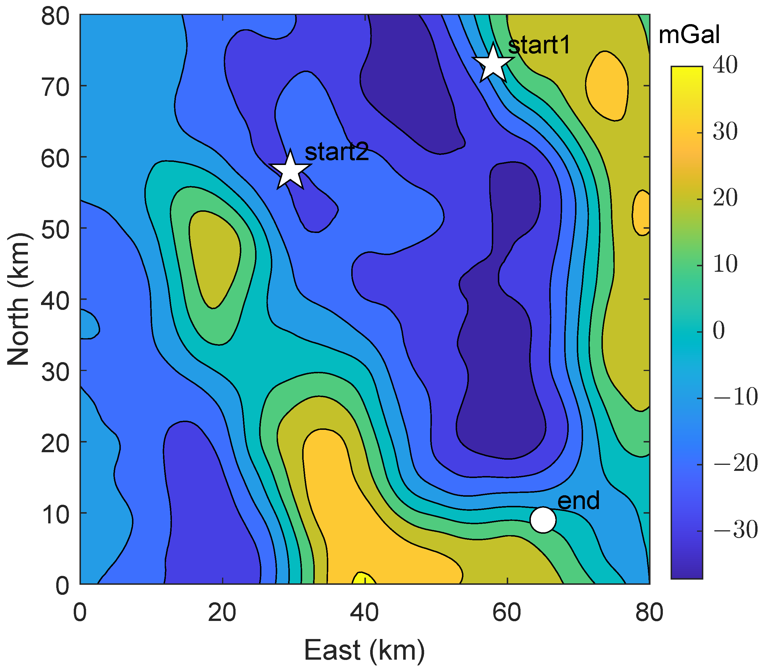
The numerical gravity map of the simulation shown in Figure 2 is derived from the global ocean gravity field $1^{\prime }\times 1^{\prime }$ model produced by Sandwell’s team [35], and the accuracy of the gravity field of the selected experimental region is better than $1.7$ mGal. The maximum gravity anomaly in the region is $40.8$ mGal and the minimum is $-37.2$ mGal. The gravity anomaly is highly undulating and contains various topographic features such as peaks, slopes, and flats, which are suitable for path planning analysis. Since the actual horizontal distances of longitude and $1^{\prime }$ latitude of $1^{\prime }$ are different, this paper projects the earth coordinate system to the geographic coordinate system, and the spatial resolution of the interpolated map is 1 km.

The measure of trajectory performance uses the Root Mean Square Error (RMSE), which is the square root of the ratio of the square of the deviation of the predicted value from the true value to the number of observations n.

$$\mathrm{RMSE}=\sqrt{\frac{1}{N}\sum _{i=1}^n\left(\left\{{\widehat{x}}_i\right\}-\left\{x_i\right\}\right)}$$

(31)

where $\left\{\widehat{x_i}\right\}$ is the estimated value of the trajectory coordinates, $\left\{x_i\right\}$ is the true value of the trajectory coordinates, and N is the number of Monte Carlo experiments.

The estimated position $\widehat{x}$ is calculated by the SITAN algorithm, which is essentially an extended Kalman filter algorithm [5,36]. The state error propagation of SITAN can be simply modeled as (32).

$$\Delta x_{t+1}=\Delta x_t+v_t$$

(32)

where $\Delta x_t$ is the position error of INS, i.e., $\widehat{x_t}=x_{\mathrm{INS}}-\Delta x_t$.

SITAN uses random linearization techniques to fit linear observation models.

$$z_t=h\left(x_t\right)-y_t\approx H\Delta x_t+\epsilon$$

(33)

where coefficients for $H=[h_{\lambda },h_{\phi }]$ can be obtained from the following

$$\begin{array}{cc}\hfill h_{\lambda }& =\frac{1}{L(2L+1)(L+1)\delta }\left(\sum _{\begin{array}{c}n=i-L\\ m=j-L\end{array}}^{\begin{array}{c}n=i-1\\ m=j+L\end{array}}\Delta g_M(n,m)-\sum _{\begin{array}{c}n=i+1\\ m=j-L\end{array}}^{\begin{array}{c}n=i+L\\ m=j+L\end{array}}\Delta g_m(n,m)\right)\hfill \end{array}$$

(34)

$$\begin{array}{cc}\hfill h_{\phi }& =\frac{1}{L(2L+1)(L+1)\delta }\left(\sum _{\begin{array}{c}n=i-L\\ m=j-L\end{array}}^{\begin{array}{c}n=i+L\\ m=j-1\end{array}}\Delta g_M(n,m)-\sum _{\begin{array}{c}n=i-L\\ m=j+1\end{array}}^{\begin{array}{c}n=i+L\\ m=j+L\end{array}}\Delta g_m(n,m)\right)\hfill \end{array}$$

(35)

(34) and (35) describe the process of calculating the observation matrix H for gravity anomaly data. The variables used are as follows: $(n,m)$, which represents the grid of the INS indicator position on the digital gravity map; $\Delta g_M=h\left(x_t\right)$, which is the gravity anomaly extracted from the digital map based on the INS indicated position; $\Delta g_m=y_t$, which is the gravity anomaly measured in real-time; $\delta$ which is the spacial resolution of the digital map; and L, which represents the number of grid points in the length of the fitted interval. Generally, a more accurate INS indicator position leads to a smaller INS confidence interval, resulting in a more precise linearized observation model.

For comparison, the following method [31,37] (hereinafter named method1) is used to calculate the informative areas.

$$\begin{array}{cc}\hfill S_{\mathrm{latitude}}=& {[g(i,j)-g(i,j-k)]}^2+{[g(i,j)-g(i,j+k)]}^2\hfill \end{array}$$

(36)

$$\begin{array}{cc}\hfill S_{\mathrm{longitude}}=& {[g(i,j)-g(i-k,j)]}^2+{[g(i,j)-g(i+k,j)]}^2\hfill \end{array}$$

(37)

$$\begin{array}{cc}\hfill \Gamma (i,j)=& \sqrt{\left(S_{\mathrm{longitude}}+S_{\mathrm{latitude}}\right)/4},\hfill \end{array}$$

(38)

where $S_{\mathrm{latitude}}$ and $S_{\mathrm{longitude}}$ are the sum of the squares of the gravity anomaly differences between point $(i,j)$ and its adjacent points within a distance of k in the latitude and longitude directions. When $k=6$, $T>9.3$ is used as a criterion for determining the informative areas, as shown in Figure 3.

In order to implement method1 in the A* algorithm, the following design was carried out:

$$H_{method1}\left(n\right)=d_g$$

(39)

$$G_{method1}\left(n\right)=\left\{\begin{array}{c}0,\mathrm{when}(\mathrm{i},\mathrm{j})\in \mathrm{informative}\mathrm{areas}\hfill \\ 1,\mathrm{when}(\mathrm{i},\mathrm{j})\in \mathrm{non}-\mathrm{informative}\mathrm{areas}\hfill \end{array}\right.$$

(40)

The meaning of (39) is to use the distance from the current point to the goal point as the heuristic function $H\left(n\right)$. (40) represents a cost function $G\left(n\right)$ of 0 in the informative areas and 1 in the non-informative areas, rather than being treated as obstacles.

4.1. Test 1

The starting point of Test 1 in the planned path is located at $(58,73)$ (start1 in Figure 2). The point is located within the slope area, where contour lines are densely distributed. The ending point, on the other hand, has coordinates of $(65,9)$.

Table 1. Simulation parameters settings.

Carrier velocity V	5 m/s
Initial position covariance $P\left(x_0\right)$	$diag\left([1,1]\right){\mathrm{km}}^2/\mathrm{s}$
Process noise covariance $Q_t$	$diag\left({[0.01,0.01]}^2\right){\mathrm{m}}^2/\mathrm{s}$
Measurement noise covariance $R_t$	$4{\mathrm{mGal}}^2$
Map Spatial Resolution $\delta$	1 km
Number of Monte Carlo runs	1000

lists the simulation conditions.

The background in Figure 4 is the $Mn$ contour filling map calculated from Equation (19) in spatial domain, i.e.,

$$M_n=\sqrt{tr\left\{H_n^T{R}_n^{-1}{H}_n\right\}}$$

(41)

where $H_n$ is the slope vector of the gravity field, and $R_n$ is the variance of the gravity measurement error at position n. $Mn$ represents the information of gravity anomaly fields in a small area that GAINS can collect. That is, a large $Mn$ means a small value of positioning error. A comparison between this and the gravity anomaly contours in Figure 2 reveals that regions with denser contours correspond to larger $Mn$, which indicates that gravity navigation is more advantageous in these areas. In addition, compared with Figure 3, areas with large $Mn$ (i.e., dark colored areas) are basically consistent with the informative areas determined by method1, indicating that $Mn$ can quantify the informative areas.

As shown in Figure 4, following the proposed method, the planned path intersects the region with maximum information. However, the trajectory planned by method1 roughly follows the contour of the informative areas, rather than the center. Furthermore, the planned trajectory is smoother than the trajectory of method1, which is beneficial for heading control. In order to determine the optimality of the planned path, in addition to the path of method1 and the shortest path, we established several equidistant curves for comparison. Five additional curves were labeled as L1, L2, … curves, L5, from left to right, with a horizontal distance of 3.5 km between them.

We conducted Monte-Carlo simulations 100 times with the same parameters as those listed in Table 1. Each trajectory was divided into 100 sampling points by equal Euclidean distances. Figure 5 provides a comparison of the localization accuracy achieved using different trajectories in Test 1. As can be seen from Figure 5, the RMSE of all paths decreases rapidly during the initial stage since the starting point 1 is located in a region with high $Mn$ values. Among them, due to L4 and L5 towards the east heading in the initial stage, where the $Mn$ value there is relatively small, there is a slower RMSE descent of the trajectory in these two compared to other trajectories. Although the planned trajectory does not maintain the lowest RMSE throughout the entire path, it can be seen in the Figure 6 that the total RMSE of the planned trajectory is the smallest.

A noteworthy phenomenon is that even though L1 deviates from areas with high $Mn$ values, or even has a segment in the trajectory that is in a very small $Mn$ region, it still achieves a lower RMSE. One possible reason is that its path is short, so the divergence of the INS is small. The positioning accuracy is the comprehensive result of INS divergence and gravity-assisted correction, which cannot be determined solely by $Mn$ or the characteristic parameters of informative areas.

4.2. Test 2

Test 1 indicates that the RMSE of all trajectories decreases rapidly during the initial phase because the starting point is located in informative areas. Test 2 changed the starting point to $(30,58)$ (start2 in Figure 2), situated at a relatively gentle seabed. As shown in Figure 7, this location has a smaller $Mn$ value, indicating that less gravity information can be used at the initial position. Consistent with test 1, in Figure 7, the black curve represents the planned trajectory, the gray curve represents the direct trajectory, and the blue curve represents the method1 trajectory. Similarly, we also designed L1–L5 as a comparison, with a horizontal spacing of approximately 5.5 km. Due to the distance from the informative areas, method1 fails at this test and only implements the shortest path planning of the A* algorithm without passing through any informative areas.

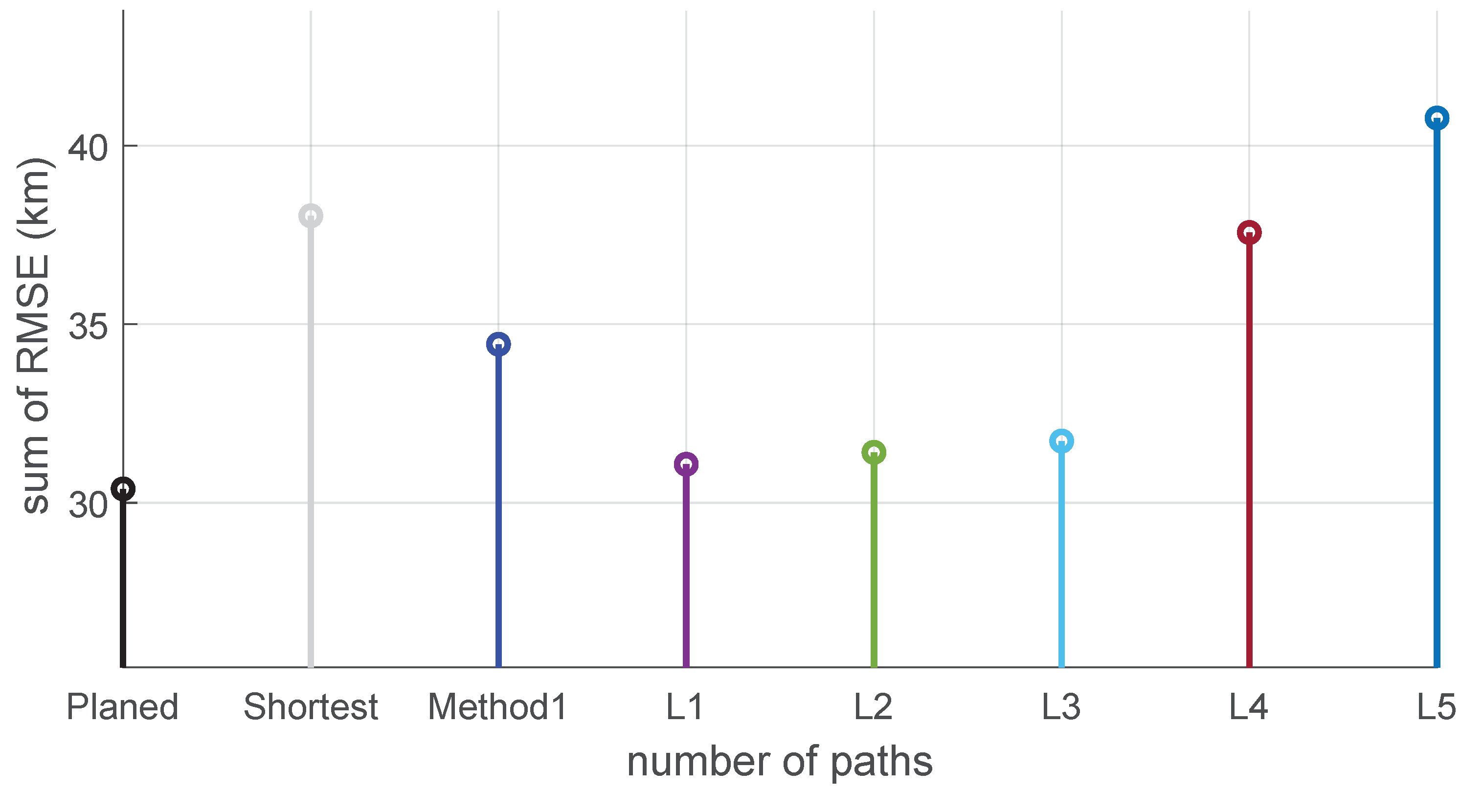
The simulation parameter settings are the same as Table 1. Figure 8 shows the RMSE of the position error for these trajectories, and the sum of RMSE values for each trajectory is presented in Figure 9.

In addition to the planned trajectory, L1, L2, and L3 all cross the area with large $Mn$ values on the left side in the initial stage, where L2 overlaps with the planned trajectory for a long time. In the magnified coordinate area, it can be seen that these four curves have a significantly faster descent speed at the beginning than the other four curves, including the straight line trajectory, method1 trajectory, L4, and L5. As shown in Figure 9, among all trajectories, the sum of RMSE for L2 and L3 is close to the planned trajectory, but their path length is longer, and the planned path is still the optimal choice. Due to the neglect of the relative value of information in the path planning method based on informative areas, available gravity information below the set threshold is discarded, and the setting of the threshold is vague and empirical, and will not be applicable to any sea area. Therefore, as shown in Figure 9, method1 exhibits the worst RMSE, even worse than the shortest path. On the contrary, the path planning method based on PCRB has clear information significance, considering not only the amount of gravity field information, but also the distance factor and INS drift rate, thus obtaining the optimal results.

4.3. The Impact of Changing the Measurement Noise on the Paths

In practice, the statistical characteristics of gyroscopes and accelerometers noise in inertial navigation systems are usually known and stable after careful calibration, so the process noise is stable. Therefore, the main factor to consider is the impact of gravity measurement errors. And since gravity measurement noise is affected by carrier motion, waves, and inaccurate map modeling, its variance is difficult to estimate accurately, so path planning should be considered to adapt to different measurement noise. The calculation of the sum of RMSE of two experimental trajectories is carried out by changing the standard deviation of the measurement noise $\sqrt{R_t}$ to obtain

Table 2. Sum of RMSE of the trajectories in Test 1.

$\sqrt{{\mathit{R}}_{\mathit{t}}}$ (mGal)	Sum of RMSE (km)
	Planned	Shortest	Method1	L1	L2	L3	L4	L5
1	18.7	25.2	21.0	19.7	19.8	20.9	25.0	27.4
2	30.4	38.0	34.4	31.1	31.4	31.7	37.6	40.8
3	53.4	67.1	56.4	57.2	55.2	58.2	66.0	69.1

.

In an overall view in Table 2 and

Table 3. Sum of RMSE of the trajectories in Test 2.

$\sqrt{{\mathit{R}}_{\mathit{t}}}$ (mGal)	Sum of RMSE (km)
	Planned	Shortest	Method1	L1	L2	L3	L4	L5
1	27.8	55.5	61.8	38.0	29.0	29.7	37.7	64.1
2	41.7	75.0	85.0	59.7	43.4	43.4	53.4	67.3
3	51.9	87.3	98.4	75.2	55.4	54.5	65.8	80.1

, increasing the amount of measurement noise will increase the lower limit of positioning error, but will not change the ranking of the lower limit size of the curve, so the planned trajectory always has higher positioning accuracy than the other curves. Therefore, the planned trajectory is always optimal. And with the increase of the measurement noise, the improvement of the localization accuracy of the planned trajectory is more obvious. The optimality of the planned trajectory is not affected by gravimetric measurements, so that the planned trajectory can be navigated in one determined ocean mission to achieve the optimal navigation accuracy. In addition, the RMSE of a spatially close trajectory to the planned path is also close to the RMSE of the planned trajectory. Therefore, even if the real path deviates from the planned one by a small amount, it is possible to obtain a high positioning accuracy by gravity information.

5. Conclusions

This article proposed a method to plan a path that aims for the best positioning accuracy by using the Postiori Cramer-Rao bound of Gravity-aided Inertial Navigation System as the cost value in the A* algorithm. This path planning method is not limited by the ocean gravity field and can plan the trajectory with the minimum navigation error between any start and end points. The next work is to find the set of trajectories within a certain error requirement in which the carrier can achieve higher positioning accuracy without strictly following a certain trajectory, thereby improving the mobility of the carrier.