1. Introduction
Optical seafloor observations, typically acquired with ROV (remotely operated vehicle), AUV (autonomous underwater vehicle), and deep-towed systems, are now routinely used in a wide range of studies and disciplines (biology, geology, archaeology, engineering, industry, etc.). Seafloor optical imagery may be processed to generate both 2D photo-mosaics and 3D terrain models, facilitating quantitative studies of the underwater environment (e.g., measuring surfaces, sizes, and volumes, among others). Textured 3D models offer a global three-dimensional view of study sites that cannot be achieved from video feedback during the dives or from other unprocessed imagery acquired by underwater vehicles.
Hence, systematic optical seafloor mapping is now routinely conducted by both ROVs and AUVs, to produce useful representations of the seafloor, either in the form of georeferenced 2D mosaics or 3D reconstructions. These representations are crucial for a better understanding of benthic processes, such as hydrothermal systems and seafloor ecosystems in general [
1,
2,
3,
4,
5,
6]. They are also widely used for other applications, such as ecology and habitat mapping [
7,
8,
9,
10,
11,
12,
13,
14] and underwater archaeology [
15,
16,
17,
18,
19], among many others. With existing algorithms (e.g., [
20]), processing can provide an optical overview of the sea floor, producing geo-localized and scaled mosaics of a limited extent. Further processing can generate maps and models of large areas of interest, which can be interpreted subsequently by users (GIS tools, ™Matlab, or other specialized software).
The 2D mosaics show limitations and distortions owing to the three-dimensional nature of submarine environments and study sites. Modeling of 3D submarine relief and large study areas requires advanced image processing expertise and involves extensive image post-processing. Specialized software is also needed to take into account the limitations and characteristics of underwater imaging, including uneven illumination and a possible lack of ambient light (e.g., in deep-sea environments), color-dependent attenuation, and inaccurate vehicle navigation, among others. Available commercial–open-source 3D reconstruction software is mostly geared towards terrestrial and sunlit scenes (e.g., aerial drones), and requires a relatively high level of user expertise to achieve good results for large scenes. Although there has been a considerable increase in the use of these tools [
21], they are generally ill-suited for submarine imagery, even when applied to shallow-water environments [
22].
This paper presents two open-source software tools designed to create and analyze 3D reconstruction models of underwater environments:
Matisse and
3DMetrics.
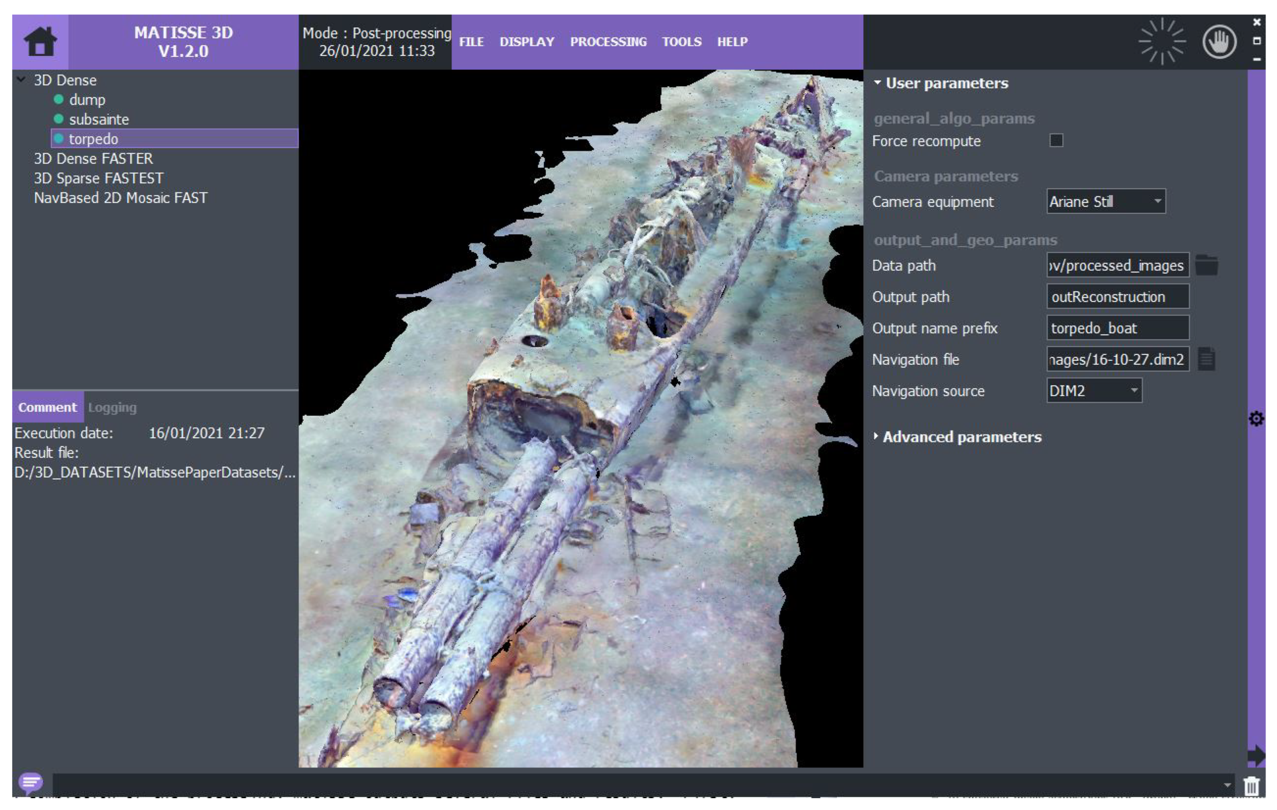
Matisse is designed for non-expert users to easily generate fully-textured high-quality 3D models from submarine optical imagery and associated navigation data (see
Figure 1 for GUI overview). Meanwhile,
3DMetrics provides a comprehensive set of tools for analyzing the geometric properties of these models.
These software tools fill an important gap in the marine science community by providing a user-friendly solution for photogrammetry-based reconstruction of benthic structures using optical marine imagery. They enable researchers to generate and analyze 3D models with ease, facilitating more accurate and efficient analysis of underwater environments.
To showcase the utility of our processing tools, we present the results on four distinct underwater datasets (see
Table 1), including raw navigation and image data, as well as the corresponding reconstructions created by
Matisse. These datasets have been acquired with state-of-the-art deep-sea vehicles used in the French Oceanographic Fleet
1 and are openly accessible to interested users for training on Matisse software, as well as for further research and comparison purposes.
Matisse and
3DMetrics are developed for both Linux and Windows operating systems, are open-source, and publicly available on GitHub:
https://github.com/IfremerUnderwater (accessed on 5 April 2023).
2. Data Acquisition and Processing Workflow
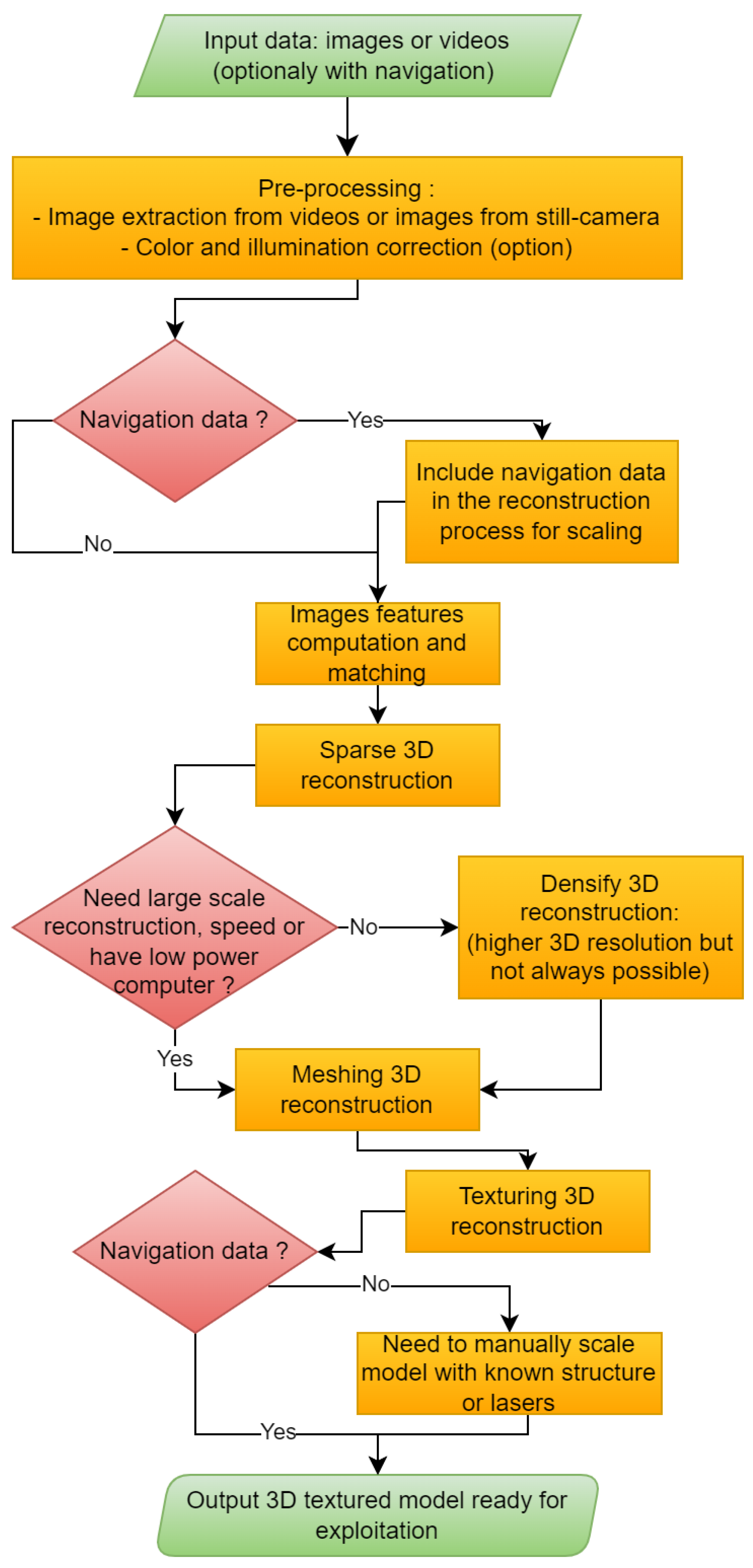
Here, we present an overview of the proposed workflow from the acquisition to visualization of 3D results, based on extensive past experience in seafloor mapping, and integrated into
Matisse software (see
Figure 2). This workflow is hardware-independent and is flexible to match available computational resources for 3D reconstruction, types of imagery and datasets, as well as final applications.
2.1. Survey Strategy for Image Acquisition and Data Requirements
During underwater surveys, image acquisition plays a crucial role in the workflow strategy to obtain 3D terrain reconstructions and texture mapping. This initial step cannot be systematically replicated, due to changes in the imaging systems, environmental conditions, illumination, geometry, the nature of surveyed objects, the type of vehicle and navigation, etc. [
23]. Differences between surveys, which impact the subsequent processing workflow, are exacerbated in submarine environments when compared to sub-aerial imagery (i.e., acquired by drone). While structure-from-motion (SfM) [
24,
25] can be applied to any optical source (photo or video) to obtain 3D optical reconstructions, particular care is needed for submarine imagery [
26].
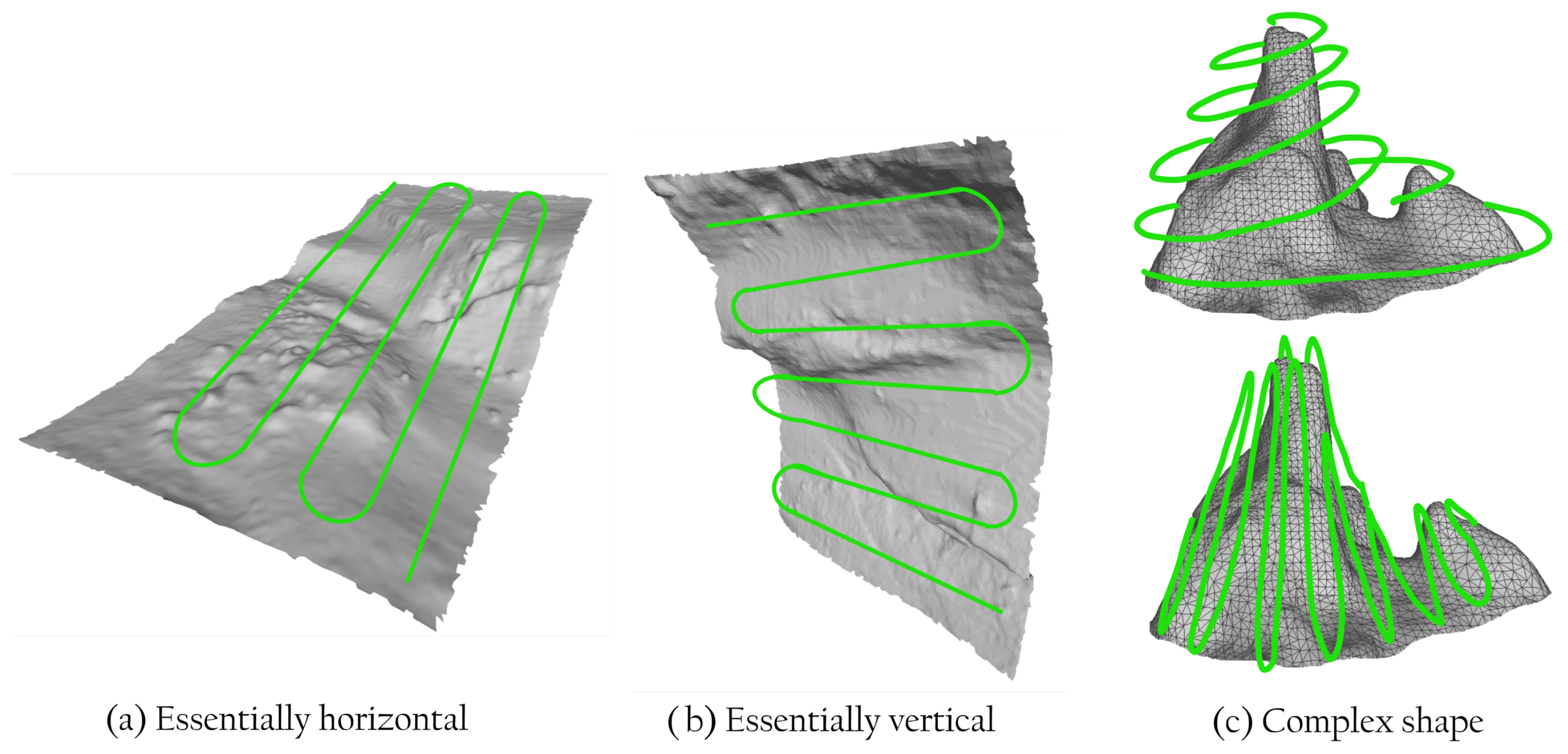
The SfM reconstruction method is based on the triangulation of points from the same scene captured from different viewpoints. In order for this to be effective images for 3D reconstruction must overlap by at least 50% in the main survey direction and for subsequent images. For robust reconstructions, points from a scene should be viewed from three viewpoints or more, increasing image overlap to 75% or better. This can be achieved by either repeated passes over the same area or surveying at low speeds (see
Figure 3 for different acquisition scenarios). These constraints weigh on the trade-off between video and still imaging. While images extracted from videos can always fulfill overlap constraints, video sensors are usually less light-sensitive and have lower resolution than still imaging sensors. On the other hand, still images often lack optimal overlap, as strobe lights impose a low frequency of acquisition (one image every few to tens of seconds). Despite this issue, still images acquired during well-planned surveys, with significant overlap, often yield the best 3D reconstruction results. This configuration is desirable but not widely used, and is not a strict requirement for 3D reconstruction.
Three-dimensional (3D) reconstruction using a single optical system (i.e., a single camera with no navigation) cannot reproduce the scene scale [
24] or its absolute orientation and position. Hence, resulting 3D models provide information on the relative size and proportion of objects, without constraints on absolute sizes. Absolute scaling and proper positioning rely on additional external data, and
Matisse can include the vehicle or platform navigation parameters in the processing pipeline (see
Figure 2), producing a scaled, oriented 3D model positioned globally. Scale accuracy will depend on the navigation quality associated with the imagery. Alternatively, in the absence of navigation data, the user may establish model scaling
a posteriori, based on known sizes of imaged objects within the 3D model, and using other tools that are able to manipulate 3D models (such as CloudCompare
2 or Meshlab
3).
The quality and limitations of available navigation data are, thus, critical factors impacting the accuracy of scaling, orientation, and the global positioning of resulting 3D models. Underwater vehicles often acquire the required navigation information (heading, roll, pitch, depth, latitude, and longitude), but navigation based on acoustic positioning, such as USBL (ultra-short baseline), is inaccurate (≈ of the water depth), and affected by noise, in addition to other biases (e.g., survey-to-survey shift, poor calibration, etc.). Acoustic navigation data may be integrated with data from other sensors, such as a bottom lock using DVL (Doppler velocity logger) systems, or inertial navigation, which are more accurate at short spatial scales but may drift over time. Different navigation data may be merged to filter noise (USBL data) and correct drift (bottom lock and inertial data). For example, surveys with no USBL data and relying on inertial navigation may yield globally distorted or wrongly oriented 3D models. The different navigation data and associated processing techniques are outside the scope of Matisse, and are dependent on the vehicles used in imaging surveys and navigation processing carried out by users. Finally, without vehicle navigation, the matching and alignment of images provide the camera navigation relative to the model, but scaling has to be done using known sizes of objects in the scene.
2.2. Image Preprocessing
The 3D reconstruction workflow is always based on image analysis. Most underwater surveys nowadays are video-based and, hence, image extraction is the first step when working with these, a feature provided in
Matisse. Extracted video images, or images from still-camera surveys, are then fed to the subsequent workflow (
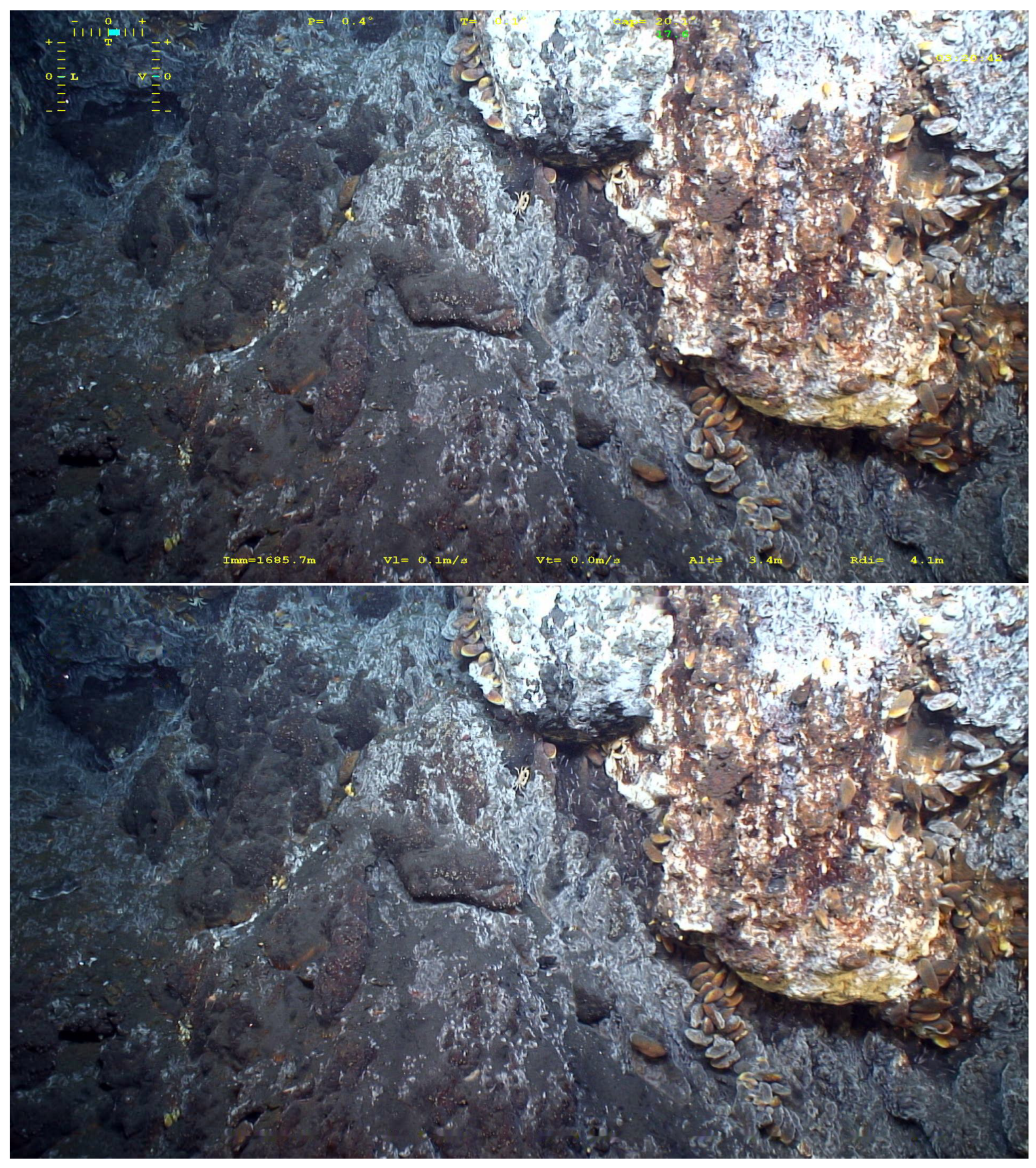
Figure 2). The 3D reconstruction may not be possible if videos or images include burnt-in text overlays (e.g., navigation time-stamps, etc.), which were common in legacy data from early surveys. To facilitate legacy data processing,
Matisse includes a tool that allows the user to inpaint [
27] input imagery to remove overlays, and it is also useful to eliminate ROV hardware within the field of view of the camera (
Figure 4).
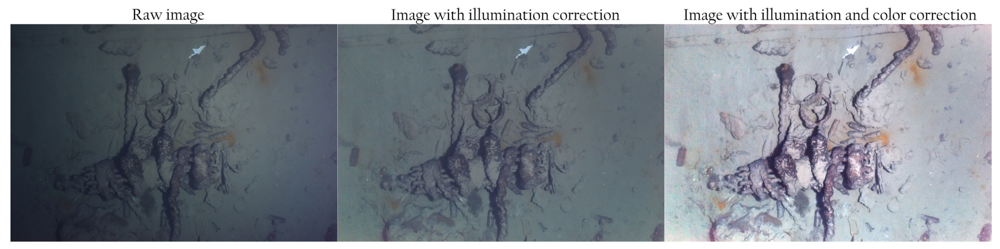
Deep underwater optical imaging is subject to quality degradation and distortion. Light attenuation is much more important underwater, compared to effects in the air, and is highly wavelength dependent. This leads to color distortion, strongly attenuating the red channel relative to the blue or green ones. Water also reflects light (backscattering), even in the absence of suspended particles, adding an undesirable background color (blue). These two effects can be corrected in Matisse by a histogram-based image saturation applied channel-by-channel (i.e., histogram stretching). The saturation of low-intensity values remove the background color, while saturation of high-intensity values corrects for attenuation.
Additional image degradation can arise from non-uniform artificial lightning. This depends on the light orientation and its projection onto the scene and may change during a survey. Uneven illumination can be corrected with an illumination pattern calculated using a temporal sliding median over subsequent images (usually three to five). To correct illumination in both video frames or still images,
Matisse inverts a paraboloid-shaped model projected on a plane [
28], a method that balances accuracy and calculation efficiency.
Figure 5 shows examples of these color and illumination corrections.
2.3. Computing 3D Textured Models
Once images have been pre-processed, the created image dataset can be fed into the 3D reconstruction pipeline, with or without navigation data. In the following, we will describe the step-by-step processing of
Matisse in accordance with the workflow depicted in
Figure 2.
2.3.1. Image Feature Computation and Matching
The first step involves the identification of features (or characteristic points) in every image. Different types of features are available in the libraries used by
Matisse, including SIFT (scale-invariant feature transform) features [
29], which have proven their robustness in underwater applications [
30,
31,
32].
Once extracted, these 2D features have to be matched between the different images in order to establish 2D–2D correspondences that will serve as the basis for the SfM processing (see
Section 2.1). This feature-matching step can be quite demanding in terms of computation, depending on the number of images to process. Both CPU and GPU implementations of SIFT are available and, thus, provide great flexibility with respect to the users’ hardware while allowing GPU-equipped users to experience substantial speed improvements.
Matisse provides several strategies to perform the matching: exhaustive, transect-based, and navigation-based.
The most basic, and computationally extensive, strategy is the exhaustive mode, which applies brute-force matching where each image is compared to every other image. To reduce the computation time, the transect- and navigation-based strategies can be used instead. The transect-based strategy is meant for sequentially acquired images and allows the user to define an overlap number N that will restrict the matching of a given image to the N following ones. On the other side, the navigation-based method takes advantage of navigation data, if available, in order to restrict the matching based on a user-defined spatial distance: that is, only the images closer than a threshold in meters are selected as matching candidates. This last strategy is the most advantageous one if navigation data are available and reliable as it greatly reduces the computation and is more likely to produce accurate matches for the SfM.
Using the identified matches and a camera model, Matisse simultaneously retrieves the camera position and orientation (i.e., the camera pose) for all images, and the 3D positions of matched points. The camera model comprises two components: a distortion model with associated parameters, and intrinsic parameters consisting of the focal length and principal point.
The best reconstruction results are achieved if intrinsic camera parameters, such as focal length, are known, so that distortions induced by the lens and viewport can be corrected geometrically.
Matisse holds the camera parameters of a selection of deep-sea research vehicles. The user can upload additional user-defined camera parameters, and obtain these using the
Matisse calibration tool.
Matisse also handles imagery acquired with an uncalibrated camera (i.e., with unknown intrinsic parameters), using the pinhole model with radial distortion, which is a widely used camera model [
24,
33].
2.3.2. Sparse 3D Reconstruction
Many techniques have been proposed to solve the SfM problem [
34,
35,
36,
37,
38,
39,
40]. Comparisons of different state-of-the-art algorithms show that they lead to very similar results in terms of accuracy (e.g., [
41]). In
Matisse, we use the
openMVG framework [
40], as it provides open-source state-of-the-art algorithms that are frequently updated following developments reported in the literature, and numerous parameters and tuning settings. One key feature of underwater imaging is its capability to optionally include the vehicle (or camera) navigation at an early stage in problem-solving, leading to the automatic scaling of the 3D model.
The result of this SfM step is the so-called sparse reconstruction. It includes only a small fraction of the scene points that can be matched and triangulated (image subsample with points that have been detected by the feature detection algorithm). This sparse reconstruction may contain holes, primarily in poorly imaged areas of the scene.
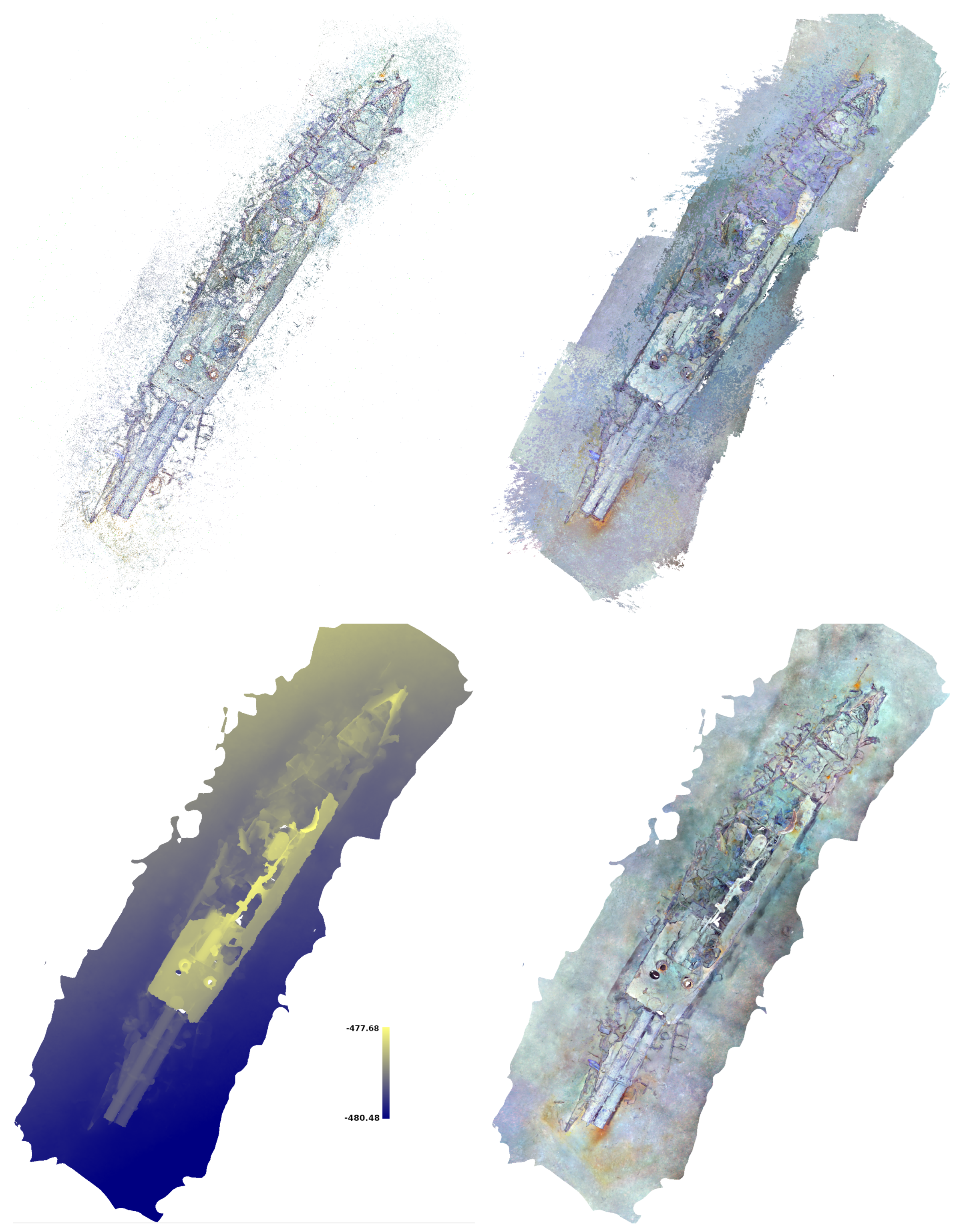
Figure 6 summarizes all the reconstruction steps, including sparse reconstruction of the torpedo ship wreck scene (
Section 4 and
Table 1).
2.3.3. Densify 3D Reconstruction
Depending on the application, the available computing power, and the need for high point density, a densification step can be applied to increase the number of reconstructed 3D points. In such cases, camera positions from the sparse reconstruction are kept fixed and a multi-view stereo technique is applied to estimate dense depth maps for each image [
42,
43,
44]. Using the camera pose and calibration estimated by the SfM, these depth maps can be projected to produce a highly dense 3D point cloud with finer geometric details than the sparse 3D reconstruction obtained solely through the SfM.
2.3.4. Meshing and Texturing
For both the sparse and densified reconstructions, the output is a 3D point cloud with camera positions. This point cloud is then meshed to recover a surface [
45], and images are projected onto the surface and blended to obtain the scene texture [
46].
In
Matisse, densification and meshing are done using the openMVS library [
47], providing both fast and close to state-of-the-art algorithms. The 3D texturing is performed with mvs-texturing [
46]. This algorithm handles large scenes that are often required in underwater studies.
2.3.5. Resulting 3D Model
Matisse produces a scaled, oriented, and georeferenced model when navigation data are provided. If navigation data are not available (and, hence, not included in the first processing steps) the final scene requires manual scaling by the user
a posteriori, using the known size of a feature in the scene, or using a laser scaler when available [
48]. The user will also need to rotate and georeference the scene based on external information. The 3D textured model obtained from either the sparse or the dense reconstruction is ready for scientific exploitation in a standard
.obj format with a geo-localization file (both in
ascii and
.kml formats).
One of the main interests of 3D textured models, in addition to reconstruction, is the possibility to carry out quantitative studies. The accuracy of scaling is difficult to establish, as it may change between surveys, and also vary within the same survey or reconstruction. While the quality of image acquisition is critical (i.e., repeated surveying of the same area, adequate distance to the scene, etc.), numerous other parameters may vary during a single survey (type of camera, availability of its model parameters, navigation quality, illumination conditions, etc.). Prior studies based on state-of-the-art deep-sea vehicles with HD cameras demonstrated reconstructions that had an accuracy of ±1 cm or better [
49,
50,
51].
3. 3DMetrics: Visualization and Interpretation/Analysis Software
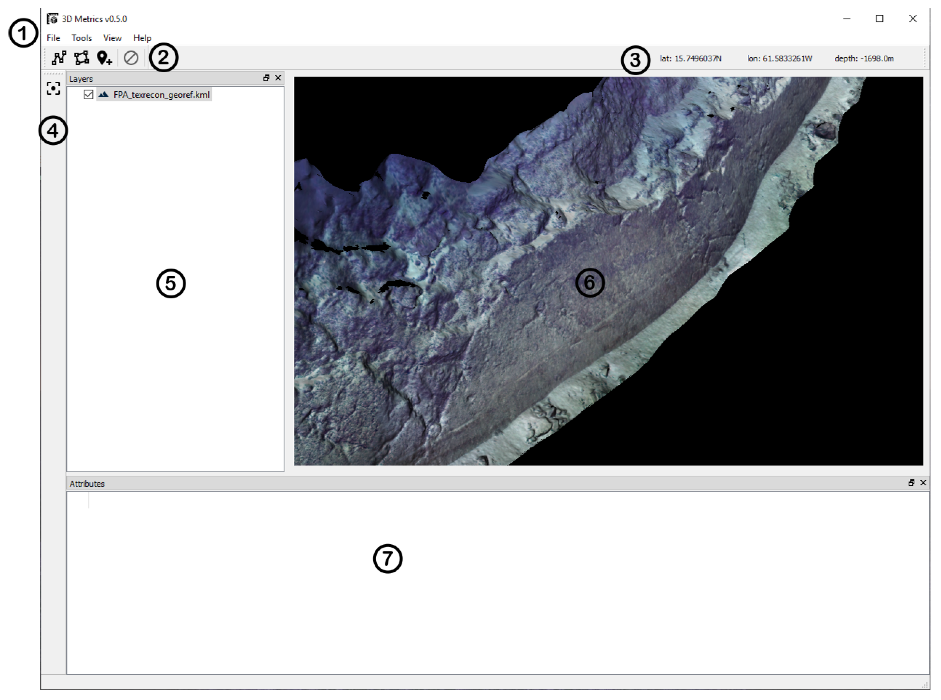
To facilitate the scientific exploitation of the results, users need software that can handle large 3D georeferenced models (including tools to interact with the scene), extract quantitative information, and manage the observations while providing input and output options. Based on experiences gained from numerous projects in different fields, we developed
3DMetrics (see
Figure 7) to accommodate some of the most common scientific needs and requirements.
3DMetrics can import both 3D and terrain models derived from optical and acoustic (multibeam bathymetry) surveys respectively. The
3DMetrics software is based on the open-source library OSG
4 and, hence, can open all formats supported by OSG. This includes the frequently used
.ply and
.obj formats, georeferenced with an associated
.kml file.
Near-seafloor optical surveys are often associated with other data (in particular, seafloor bathymetry), which provide geological and regional contexts for higher-resolution optical surveys, which are often restricted to smaller areas. Digital terrain grids in the NetCdf file format (e.g., .grd), are common and supported by 3DMetrics. Once opened, models can be manually shifted to finely co-register different datasets, as vertical and horizontal shifts of data may be required due to scale and navigation differences among datasets. This allows for the integration of different datasets, and their analyses at larger spatial scales (acoustic data) than those of optical data (3D scene) alone. The 3DMetrics software can upload several 3D models, with limitations on the number and size depending on video card hardware. To facilitate visualization of datasets, particularly with several 3D scenes viewed simultaneously, 3DMetrics constructs multi-resolution models from the original ones generated by Matisse. This feature reduces memory requirements during visualization and allows efficient data upload and rendering.
Imported 3D models can be vertically projected to create both ortho-photos and digital elevation models, exported as standard GeoTIFF files. In the released datasets, we provide ortho-photos of each resulting 3D model. This option facilitates data analyses and correlations with other 2D datasets, and the manipulation of results in other software (e.g., GIS).
In addition to visualization, the user can perform measurements on the 3D models for quantitative studies in two different modes. The ’quick measurement’ toolbar (area 2 in
Figure 7) provides interactive measurements (line, surface, point measurements), with a screen display of values that are not saved. This feature is useful to explore models, to obtain an overview of the size of the scene elements, or to pick the geographic coordinates of interest points. The second mode, best suited for quantitative studies, creates measurement layers (in area 5 in
Figure 7), allowing the user to record, save, open, and modify data. As is the standard for other types of 2D GIS software (e.g.,
ArcView,
QGIS), the measurement layer is customizable and includes user-defined attributes: line, area, point, text, and category.
The layer attribute values are stored and shown in the attribute table (area 7 in
Figure 7). The strength of 3DMetrics software is its ability to save the entire user workspace in a variety of formats, including shapefiles, text, and custom formats. This feature allows users to easily pick up where they left off in previous sessions by reopening their workspace in the exact same state.
4. Examples and Datasets: Anthropogenic, Geological, and Biological Studies
Here, we present four datasets, which were processed with
Matisse to generate 3D reconstructions: a litter dump at the seafloor, a sub-vertical fault scarp, a hydrothermal vent edifice, and a shipwreck (
Table 1). The datasets were acquired with different vehicles and camera types, and correspond to different survey patterns. The data are provided in open-access (
Table 1) and include input data (images or videos and navigation files) and the 3D models generated by
Matisse together with the corresponding ortho-photos GeoTIFF.
Table 1 provides details for each study area, including survey information, input data, output models, CPU computation time, and computer information. The choice of examples seeks to illustrate (a) different survey strategies and patterns adapted to the scene of interest, (b) imagery of varying quality and with different illuminations, and (c) examples that are relevant to different scientific disciplines (geology, archaeology, environmental studies, and biology, among others). These datasets are suitable for training and testing the different parameters and options of
Matisse, and to allow non-expert users to further explore the functionalities and parameters. All datasets were processed using color and illumination correction, the 3D dense algorithm, the SIFT CPU implementation, and the exhaustive matching strategy (i.e., brute-force matching). The first dataset was both processed with and without pre-processing to demonstrate how this correction impacts the result. The hydrothermal vent dataset includes already pre-processed images.
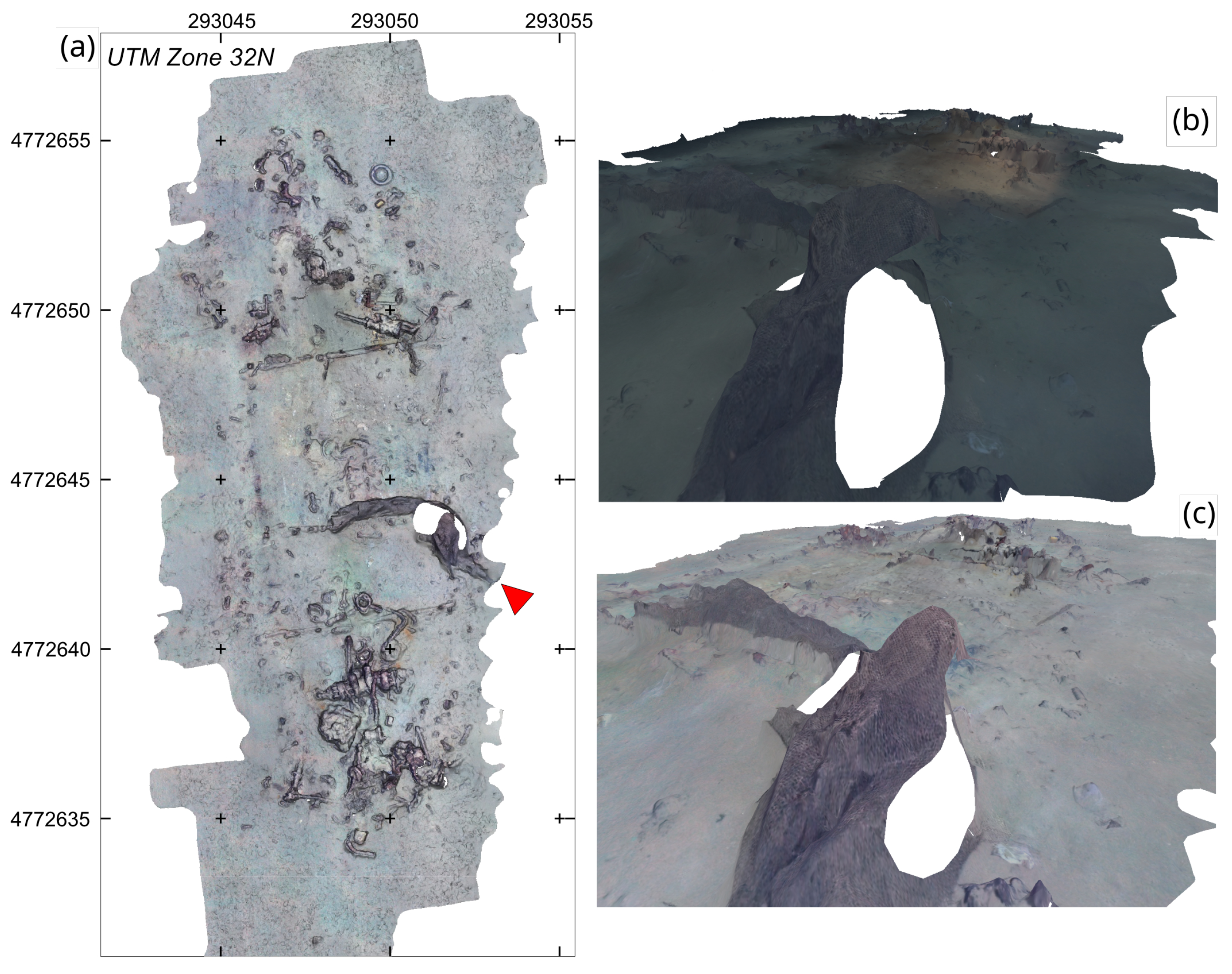
4.1. Anthropogenic Seafloor Litter Dump
The first example corresponds to anthropogenic litter and debris off the French Mediterranean coast (43.078° N; 6.458° E), at a water depth of ≈600 m, acquired during the technical CARTOHROV-GEN cruise.
With
Matisse, we generated two final dense 3D-textured models, with uncorrected and corrected color and illumination, and an additional sparse model (see
Table 1). The corrected imagery greatly improves the quality of the resulting 3D terrain model, with a rendering that facilitates its interpretation relative to the model derived from uncorrected data.
Figure 8 shows the orthophotomosaic, and a scene detail shows the difference between using images that are uncorrected and corrected for illumination.
This dataset corresponds to a sub-horizontal scene and may be applicable to many geological, biological, and environmental studies (e.g., distribution of seafloor ecosystems, fluid outflow at hydrothermal vents and cold seeps, etc.). Numerous studies have investigated seafloor litter from visual observations [
52,
53,
54], and quantification is typically based on the occurrence of objects along deep-sea vehicle tracks [
55,
56]. Proper quantitative studies can only be achieved with 2D and 3D photomosaics, which provide a comprehensive view of selected seafloor areas and where a proper quantification of the density of objects can be established from extensive image surveys. These datasets are also suitable for temporal studies that are not feasible with along-track imagery alone, owing to the difficulty of precisely collocating individual ROV tracks acquired at different times. Instead, repeated surveys of a given area ensure both the overlap of imaged areas, and the adequate co-registration required for such quantitative studies. This approach has been successfully applied to monitor temporal variations in cold seeps, active hydrothermal systems, or impact studies [
4,
6,
57], among other environments.
4.2. Fault Scarp and Associated Tectonic Markers
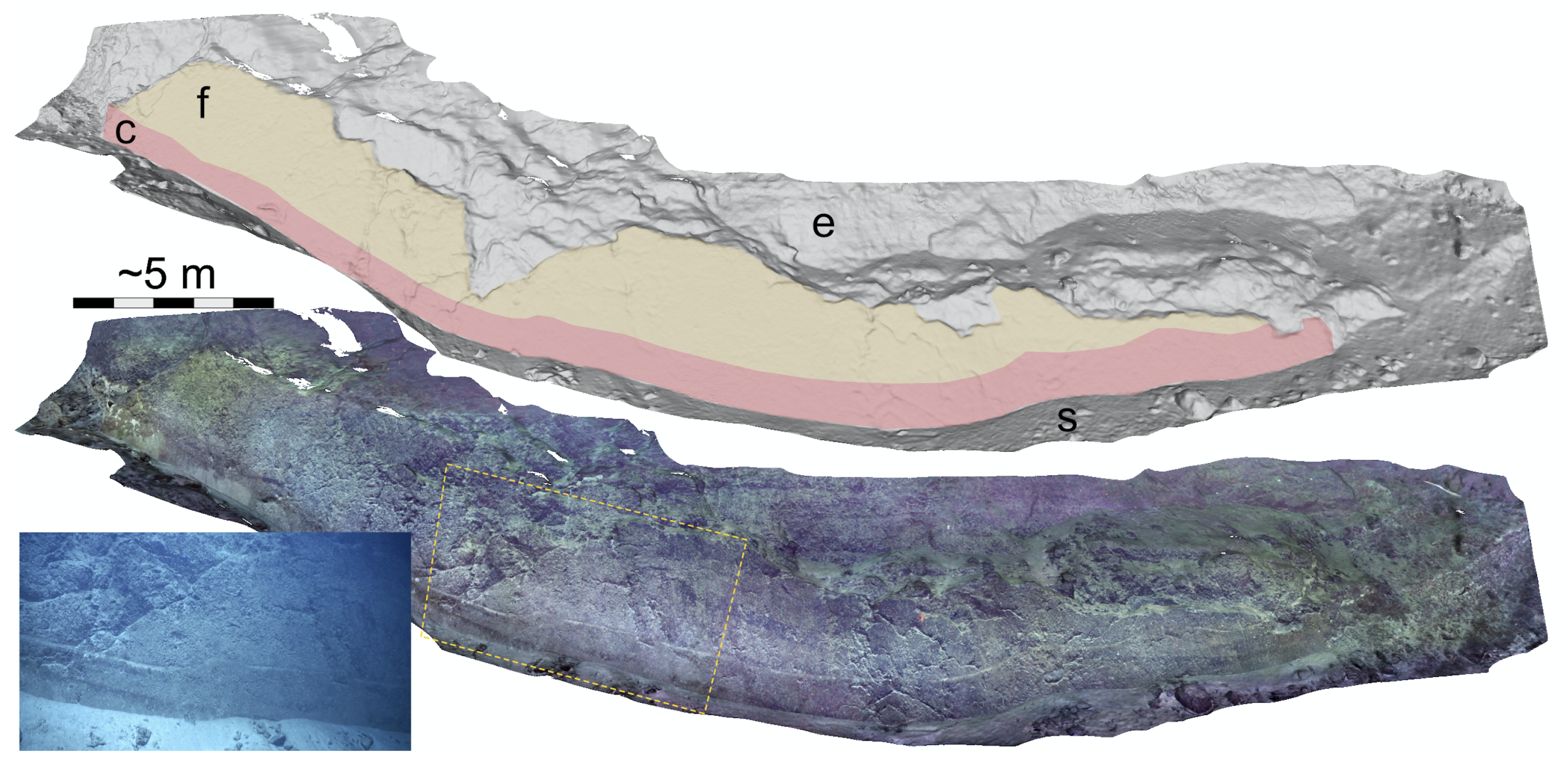
Our second example corresponds to a video sequence of a submarine fault outcrop displaying markers of a past seismic event. This outcrop is located along the Roseau Fault, between the Les Saintes and Dominica islands (Lesser Antilles), which ruptured during the 2004 Les Saintes Earthquake. Data were acquired during the SUBSAINTES 2017 cruise, using an HD video camera mounted on the Victor 6000 ROV. The 3D model revealed the traces of this seismic event in the fault scarp, which were not readily identifiable in the original video imagery [
58].
Figure 9 shows the overall fault scarp, where the well-preserved fault plane is clearly identifiable as a smooth, sub-vertical surface emerging from the seafloor. On the flanks and above this plane, the irregular surface texture is the associated fault plane degradation. A band at the base of the scarp mimics the geometry of the contact between the fault plane and the present-day seafloor. This band is a freshly exposed, uneroded scarp that recorded the recent 2004 earthquake [
58]. These reconstructions allow for quantitative studies (here, the earthquake-induced vertical fault displacement), based on measurements over the 3D scene, and with a resolution of 1 cm or better. These observations may also be critical to document temporal changes (future seismic slip events, as well as erosion and sedimentation processes at the scene).
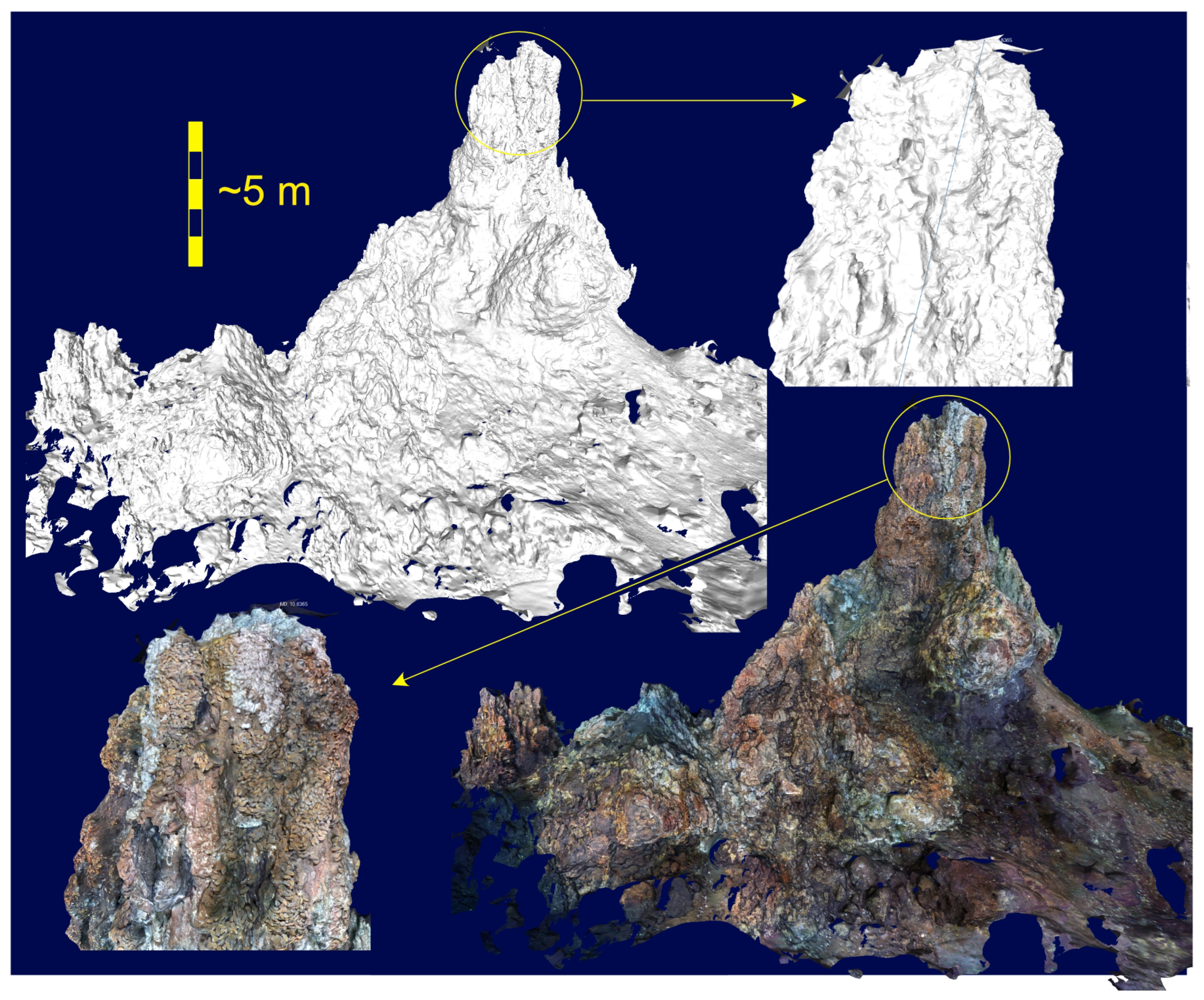
4.3. Hydrothermal Vent Edifice
Our third example is a well-studied hydrothermal chimney, the Eiffel Tower, from the Lucky Strike hydrothermal field along the Mid-Atlantic Ridge, acquired during Momarsat2015 cruise. This massive sulfide edifice was built from the long-term precipitation of polymetallic sulfides contained in high-temperature fluids (>300 °C) and rises 15–20 m above the surrounding seafloor. Macrofaunal communities, dominated by dense mussel beds of Bathymodiolus azoricus, and microbial mats colonize large areas of its walls.
The original video stream included burn-in text overlays. Prior to processing, we extracted video frames and removed the text by inpainting (see
Section 2.2 and
Figure 4) with
Matisse. Without processing, these annotations may result in lower-quality models or a failure of the processing. Inpainting is preferred to image cropping as it keeps most of the information that was within the original image. It also ensures that the center of the image before and after is not modified and, therefore, that the optical center of the image stays close to the image center. Cropping is not recommended as it usually modifies the image and optical centers. The Eiffel Tower input dataset includes 4875 images from video frame extractions, with a subset of images associated with navigation, and a subset without navigation. The model extends ∼
m horizontally and 20 m vertically, over a total surface of 920 m
.
Ecosystems are often hosted in geometrically complex habitats, which can be linked to a wide range of faunal and microbial communities. Moreover, 3D models are critical to understanding these habitats, communities, species distributions, and associated environmental drivers. The resolution of this texture-mapped model (
Figure 10) allows for the identification of fauna assemblages and substrate types, which can be mapped to understand community structures at small spatial scales [
1,
59]. Successive surveys and resulting 3D models at adequate time scales provide a unique opportunity to study fine temporal variations. The Eiffel Tower hydrothermal chimney, and its faunal and microbial communities, were mapped in 2015 (this dataset) and 2016, with additional models acquired in 2018 and 2020 being processed for temporal studies. Similar 3D temporal studies have been conducted in other ecosystems [
57,
60]. Finally, the 3D model was also used from year to year to relocate the ROV through the comparison with live video streams and facilitate the installation of measurement equipment [
61].
4.4. Torpedo Boat Wreck
Underwater 3D reconstructions are often used in submarine archaeology to study shipwrecks, including the
HMS Titanic [
62], the
La Lune [
16], the Xelendi Phoenician shipwreck [
18], among many others. These 3D models are useful for planning and conducting archaeological work, documenting sites, and following their time evolution for heritage preservation and management (looting, degradation, sedimentation, etc.).
Shipwreck images were collected using HROV Ariane, off the Mediterranean coast, during the cruise CANHROV. Ariane was equipped with an electronic still camera, and navigated around the torpedo boat shipwreck, a battleship that sank in 1903 [
63] at a water depth of 476 m off the southern French Mediterranean coast (43.124° N; 6.523° E). This shipwreck was ∼20 m long and 3 m wide, rising ∼2 m above the surrounding seafloor.
Figure 6 shows the different stages of 3D reconstruction for this shipwreck scene.
5. Conclusions and Perspectives
Matisse provides a complete suite to pre-process and process underwater imagery (video and still images), and to generate 3D textured scenes. With 3DMetrics, users can visualize these 3D scenes, integrate additional data, such as other scenes and bathymetry, and extract quantitative information while providing data management capabilities and standard output options for further analyses. The processing pipeline in Matisse is specifically tailored for underwater applications, and the software development has benefited from extensive testing on numerous cruises and under various surveying scenarios. This software is designed with flexibility in mind, allowing it to be applied to various instruments and vehicles, including legacy data.
We additionally provide four open-access datasets, with explanations of the processing steps in Matisse, and the resulting 3D textured models. These different datasets are relevant for environmental impacts and pollution studies, tectonics, geology, biology, and archaeology, and this software may be used in other fields. These datasets also provide different survey configurations, illumination characteristics, and types of imagery, to showcase the flexibility and robustness of Matisse, and facilitate training.
We released a stable version of Matisse as open-source code available on GitHub, which can be installed easily on Linux and Windows systems. Future versions and updates will also be distributed through the GitHub repositories, including an OSX version, and a version specific for servers, to provide remote (client/server approach) processing capabilities. The processing time will be updated to reflect the latest hardware architecture performance as soon as possible.
Currently, 3D reconstructions are limited to scenes of a few hundred square meters due to computational and memory constraints. However, we plan to expand the scale of feasible reconstructions and increase speed by implementing smart sub-scene segmentation and fusion. As we move forward, we anticipate better integration of optical mapping with other techniques, such as multibeam high-resolution terrain data, hyperspectral imaging [
64], structured light, and underwater lidar to better characterize seafloor texture and nature. It is important to note that the limitations of reconstruction will vary depending on the survey techniques and instrumentation used, requiring a case-by-case evaluation [
26]. Nevertheless, our datasets demonstrate the flexibility and robustness of our approach.
Author Contributions
The paper was planned and coordinated by A.A. and J.E.; A.A. built upon prior software developments of Matisse and 3DMetrics. The implementation of the processing pipeline was carried out by M.F. with valuable input from N.G. and J.E. Financial support for the project was provided to A.A. and J.E. through an ANR grant. Datasets, testing, and interpretations were performed by A.A., M.F., N.G., J.E. and M.M. The writing process was coordinated by A.A. and J.E., with valuable contributions from N.G., M.F., J.O. and M.M. All authors have read and agreed to the published version of the manuscript.
Funding
The development of the software and processing of the data were partially supported by the Ifremer PSI grant scheme (3DMetrics) awarded to A.A. and M.M., as well as the ANR Sersurf (ANR-17-687 CE31-0020, PI JE) granted to A.A. and J.E. Furthermore, J.E. received support from CNRS/INSU for data exploitation during the SUBSAINTES’17 cruise. Part of the work was supported by the European Union’s Horizon 2020 research and innovation project iAtlantic under Grant Agreement No. 818123.
Informed Consent Statement
Informed consent was obtained from all subjects involved in the study.
Data Availability Statement
The data presented in this study are openly available with links described and available in the paper.
Conflicts of Interest
The authors declare no conflict of interest.
References
- Girard, F.; Sarrazin, J.; Arnaubec, A.; Cannat, M.; Sarradin, P.M.; Wheeler, B.; Matabos, M. Currents and topography drive assemblage distribution on an active hydrothermal edifice. Prog. Oceanogr. 2020, 187, 102397. [Google Scholar] [CrossRef]
- Gerdes, K.; Martínez Arbizu, P.; Schwarz-Schampera, U.; Schwentner, M.; Kihara, T.C. Detailed Mapping of Hydrothermal Vent Fauna: A 3D Reconstruction Approach Based on Video Imagery. Front. Mar. Sci. 2019, 6, 96. [Google Scholar] [CrossRef]
- Garcia, R.; Gracias, N.; Nicosevici, T.; Prados, R.; Hurtos, N.; Campos, R.; Escartin, J.; Elibol, A.; Hegedus, R. Exploring the Seafloor with Underwater Robots: Land, Sea & Air. In Computer Vision in Vehicle Technology: Land, Sea & Air; John Wiley & Sons Ltd.: Hoboken, NJ, USA, 2017; pp. 75–99. [Google Scholar] [CrossRef]
- Barreyre, T.; Escartín, J.; Garcia, R.; Cannat, M.; Mittelstaedt, E.; Prados, R. Structure, temporal evolution, and heat flux estimates from the Lucky Strike deep-sea hydrothermal field derived from seafloor image mosaics. Geochem. Geophys. Geosyst. 2012, 13, Q04007. [Google Scholar] [CrossRef]
- Thornton, B.; Bodenmann, A.; Pizarro, O.; Williams, S.B.; Friedman, A.; Nakajima, R.; Takai, K.; Motoki, K.; Watsuji, T.o.; Hirayama, H.; et al. Biometric assessment of deep-sea vent megabenthic communities using multi-resolution 3D image reconstructions. Deep Sea Res. Part I Oceanogr. Res. Pap. 2016, 116, 200–219. [Google Scholar] [CrossRef]
- Lessard-Pilon, S.; Porter, M.D.; Cordes, E.E.; MacDonald, I.; Fisher, C.R. Community composition and temporal change at deep Gulf of Mexico cold seeps. Deep Sea Res. Part II Top. Stud. Oceanogr. 2010, 57, 1891–1903. [Google Scholar] [CrossRef]
- Williams, S.; Pizarro, O.; Jakuba, M.; Johnson, C.; Barrett, N.; Babcock, R.; Kendrick, G.; Steinberg, P.; Heyward, A.; Doherty, P.; et al. Monitoring of Benthic Reference Sites: Using an Autonomous Underwater Vehicle. IEEE Robot. Autom. Mag. 2012, 19, 73–84. [Google Scholar] [CrossRef]
- Bryson, M.; Johnson-Roberson, M.; Pizarro, O.; Williams, S. Repeatable Robotic Surveying of Marine Benthic Habitats for Monitoring Long-term Change. In Proceedings of the Workshop on Robotics for Environmental Monitoring at Robotics: Science and Systems (RSS), Sydney, NSW, Australia, 9–13 July 2012. [Google Scholar]
- Gintert, B.E.; Manzello, D.P.; Enochs, I.C.; Kolodziej, G.; Carlton, R.; Gleason, A.C.R.; Gracias, N. Marked annual coral bleaching resilience of an inshore patch reef in the Florida Keys: A nugget of hope, aberrance, or last man standing? Coral Reefs 2018, 37, 533–547. [Google Scholar] [CrossRef]
- Pedersen, N.; Edwards, C.; Eynaud, Y.; Gleason, A.; Smith, J.; Sandin, S. The influence of habitat and adults on the spatial distribution of juvenile corals. Ecography 2019, 42, 1703–1713. [Google Scholar] [CrossRef]
- Rossi, P.; Ponti, M.; Righi, S.; Castagnetti, C.; Simonini, R.; Mancini, F.; Agrafiotis, P.; Bassani, L.; Bruno, F.; Cerrano, C.; et al. Needs and Gaps in Optical Underwater Technologies and Methods for the Investigation of Marine Animal Forest 3D-Structural Complexity. Front. Mar. Sci. 2021, 8, 171. [Google Scholar] [CrossRef]
- Svennevig, K.; Guarnieri, P.; Stemmerik, L. From oblique photogrammetry to a 3D model – Structural modeling of Kilen, eastern North Greenland. Comput. Geosci. 2015, 83, 120–126. [Google Scholar] [CrossRef]
- Grohmann, C.H.; Garcia, G.P.B.; Affonso, A.A.; Albuquerque, R.W. Dune migration and volume change from airborne LiDAR, terrestrial LiDAR and Structure from Motion-Multi View Stereo. Comput. Geosci. 2020, 143, 104569. [Google Scholar] [CrossRef]
- Kwasnitschka, T.; Hansteen, T.; Devey, C.; Kutterolf, S. Doing Fieldwork on the Seafloor: Photogrammetric Techniques to yield 3D Visual Models from ROV Video. Comput. Geosci. 2013, 52, 218–226. [Google Scholar] [CrossRef]
- Ballard, R.D.; Stager, L.E.; Master, D.; Yoerger, D.; Mindell, D.; Whitcomb, L.; Singh, H.; Piechota, D. Iron age shipwrecks in deep water off Ashkelon, Israel. Am. J. Archaeol. 2002, 106, 151–168. [Google Scholar] [CrossRef]
- Gracias, N.; Ridao, P.; Garcia, R.; Escartin, J.; L’Hour, M.; Cibecchini, F.; Campos, R.; Carreras, M.; Ribas, D.; Palomeras, N.; et al. Mapping the Moon: Using a lightweight AUV to survey the site of the 17th century ship ‘La Lune’. In Proceedings of the 2013 MTS/IEEE OCEANS, Bergen, Norway, 10–14 June 2013; IEEE: Piscataway, NJ, USA, 2013; pp. 1–8. [Google Scholar] [CrossRef]
- Mertes, J.; Thomsen, T.; Gulley, J. Evaluation of Structure from Motion Software to Create 3D Models of Late Nineteenth Century Great Lakes Shipwrecks Using Archived Diver-Acquired Video Surveys. J. Marit. Archaeol. 2014, 9, 173–189. [Google Scholar] [CrossRef]
- Drap, P.; Merad, D.; Hijazi, B.; Gaoua, L.; Nawaf, M.; Saccone, M.; Chemisky, B.; Seinturier, J.; Sourisseau, J.C.; Gambin, T.; et al. Underwater Photogrammetry and Object Modeling: A Case Study of Xlendi Wreck in Malta. Sensors 2015, 15, 30351–30384. [Google Scholar] [CrossRef] [PubMed]
- Fabri, M.C.; Vinha, B.; Allais, A.G.; Bouhier, M.E.; Dugornay, O.; Gaillot, A.; Arnaubec, A. Evaluating the ecological status of cold-water coral habitats using non-invasive methods: An example from Cassidaigne canyon, northwestern Mediterranean Sea. Prog. Oceanogr. 2019, 178, 102172. [Google Scholar] [CrossRef]
- Marcon, Y.; Sahling, H.; Bohrmann, G. LAPM: A tool for underwater Large-Area Photo-Mosaicking. Geosci. Instrum. Methods Data Syst. Discuss. 2013, 3, 127–156. [Google Scholar] [CrossRef]
- Pulido Mantas, T.; Roveta, C.; Calcinai, B.; di Camillo, C.G.; Gambardella, C.; Gregorin, C.; Coppari, M.; Marrocco, T.; Puce, S.; Riccardi, A.; et al. Photogrammetry, from the Land to the Sea and Beyond: A Unifying Approach to Study Terrestrial and Marine Environments. J. Mar. Sci. Eng. 2023, 11, 759. [Google Scholar] [CrossRef]
- Marre, G.; Holon, F.; Luque, S.; Boissery, P.; Deter, J. Monitoring Marine Habitats With Photogrammetry: A Cost-Effective, Accurate, Precise and High-Resolution Reconstruction Method. Front. Mar. Sci. 2019, 6, 276. [Google Scholar] [CrossRef]
- Lochhead, I.; Hedley, N. Evaluating the 3D Integrity of Underwater Structure from Motion Workflows. Photogramm. Rec. 2022, 37, 35–60. [Google Scholar] [CrossRef]
- Hartley, R.I.; Zisserman, A. Multiple View Geometry in Computer Vision, 2nd ed.; Cambridge University Press: Cambridge, UK, 2004; ISBN 0521540518. [Google Scholar]
- Ma, Y.; Soatto, S.; Kosecka, J.; Sastry, S.S. An Invitation to 3-D Vision: From Images to Geometric Models; Interdisciplinary Applied Mathematics; Springer: New York, NY, USA, 2004. [Google Scholar] [CrossRef]
- Wright, A.E.; Conlin, D.L.; Shope, S.M. Assessing the Accuracy of Underwater Photogrammetry for Archaeology: A Comparison of Structure from Motion Photogrammetry and Real Time Kinematic Survey at the East Key Construction Wreck. J. Mar. Sci. Eng. 2020, 8, 849. [Google Scholar] [CrossRef]
- Telea, A. An Image Inpainting Technique Based on the Fast Marching Method. J. Graph. Tools 2004, 9, 23–34. [Google Scholar] [CrossRef]
- Arnaubec, A.; Opderbecke, J.; Allais, A.; Brignone, L. Optical mapping with the ARIANE HROV at IFREMER: The MATISSE processing tool. In Proceedings of the OCEANS 2015, Genova, Italy, 18–21 May 2015; pp. 1–6. [Google Scholar] [CrossRef]
- Lowe, D.G. Distinctive Image Features from Scale-Invariant Keypoints. Int. J. Comput. Vis. 2004, 60, 91–110. [Google Scholar] [CrossRef]
- Ansari, S. A Review on SIFT and SURF for Underwater Image Feature Detection and Matching. In Proceedings of the 2019 IEEE International Conference on Electrical, Computer and Communication Technologies (ICECCT), Coimbatore, India, 20–22 February 2019; pp. 1–4. [Google Scholar] [CrossRef]
- Hernández Vega, J.; Istenič, K.; Gracias, N.; Palomeras, N.; Campos, R.; Vidal Garcia, E.; Garcia, R.; Carreras, M. Autonomous Underwater Navigation and Optical Mapping in Unknown Natural Environments. Sensors 2016, 16, 1174. [Google Scholar] [CrossRef]
- Garcia, R.; Gracias, N. Detection of interest points in turbid underwater images. In Proceedings of the IEEE/MTS OCEANS2011, Santander, Spain, 6–9 June 2011; IEEE: Piscataway, NJ, USA, 2011. [Google Scholar]
- Kannala, J.; Brandt, S.S. A generic camera model and calibration method for conventional, wide-angle, and fish-eye lenses. IEEE Trans. Pattern Anal. Mach. Intell. 2006, 28, 1335–1340. [Google Scholar] [CrossRef]
- Agarwal, S.; Furukawa, Y.; Snavely, N.; Simon, I.; Curless, B.; Seitz, S.M.; Szeliski, R. Building rome in a day. Commun. ACM 2011, 54, 105–112. [Google Scholar] [CrossRef]
- Schonberger, J.L.; Frahm, J.M. Structure-from-motion revisited. In Proceedings of the IEEE Conference on Computer Vision and Pattern Recognition, Las Vegas, NV, USA, 27–30 June 2016; pp. 4104–4113. [Google Scholar]
- Sweeney, C.; Hollerer, T.; Turk, M. Theia: A fast and scalable structure-from-motion library. In Proceedings of the 23rd ACM International Conference on Multimedia, Brisbane, Australia, 26–30 October 2015; pp. 693–696. [Google Scholar]
- Heinly, J.; Schonberger, J.L.; Dunn, E.; Frahm, J.M. Reconstructing the world* in six days*(as captured by the yahoo 100 million image dataset). In Proceedings of the IEEE Conference on Computer Vision and Pattern Recognition, Boston, MA, USA, 7–12 June 2015; pp. 3287–3295. [Google Scholar]
- Wu, C. VisualSFM: A Visual Structure from Motion System. 2011. Available online: http://www.cs.washington.edu/homes/ccwu/vsfm (accessed on 5 April 2023).
- Rupnik, E.; Daakir, M.; Pierrot Deseilligny, M. MicMac—A free, open-source solution for photogrammetry. Open Geospat. Data Softw. Stand. 2017, 2, 1–9. [Google Scholar] [CrossRef]
- Moulon, P.; Monasse, P.; Perrot, R.; Marlet, R. Openmvg: Open multiple view geometry. In Proceedings of the International Workshop on Reproducible Research in Pattern Recognition, Cancún, Mexico, 4 December 2016; Springer: Berlin/Heidelberg, Germany, 2016; pp. 60–74. [Google Scholar]
- Bianco, S.; Ciocca, G.; Marelli, D. Evaluating the Performance of Structure from Motion Pipelines. J. Imaging 2018, 4, 98. [Google Scholar] [CrossRef]
- Hirschmüller, H.; Buder, M.; Ernst, I. Memory Efficient Semi-Global Matching. Remote Sens. Spat. Inf. Sci. 2012, I-3, 371–376. [Google Scholar] [CrossRef]
- Barnes, C.; Shechtman, E.; Finkelstein, A.; Goldman, D.B. PatchMatch: A Randomized Correspondence Algorithm for Structural Image Editing. ACM Trans. Graph. (Proc. SIGGRAPH) 2009, 28, 24. [Google Scholar] [CrossRef]
- Shen, S. Accurate Multiple View 3D Reconstruction Using Patch-Based Stereo for Large-Scale Scenes. IEEE Trans. Image Process. 2013, 22, 1901–1914. [Google Scholar] [CrossRef] [PubMed]
- Jancosek, M.; Pajdla, T. Exploiting Visibility Information in Surface Reconstruction to Preserve Weakly Supported Surfaces. Int. Sch. Res. Not. 2014, 2014, 798595. [Google Scholar] [CrossRef] [PubMed]
- Waechter, M.; Moehrle, N.; Goesele, M. Let There Be Color! Large-Scale Texturing of 3D Reconstructions. In Proceedings of the Computer Vision—ECCV 2014, Zurich, Switzerland, 6–12 September 2014; Fleet, D., Pajdla, T., Schiele, B., Tuytelaars, T., Eds.; Lecture Notes in Computer Science. Springer International Publishing: Cham, Switzerland, 2014; pp. 836–850. [Google Scholar] [CrossRef]
- Cernea, D. OpenMVS: Multi-View Stereo Reconstruction Library. Available online: https://github.com/cdcseacave/openMVS (accessed on 5 April 2023).
- Istenic, K.; Gracias, N.; Arnaubec, A.; Escartin, J.; Garcia, R. Scale estimation of structure from motion based 3D models using laser scalers in underwater scenarios. ISPRS J. Photogramm. Remote Sens. 2020, 159, 13–25. [Google Scholar] [CrossRef]
- Istenic, K.; Gracias, N.; Arnaubec, A.; Escartin, J.; Garcia, R. Remote sensing Scale Accuracy Evaluation of Image-Based 3D Reconstruction Strategies Using Laser Photogrammetry. Remote Sens. 2019, 11, 2093. [Google Scholar] [CrossRef]
- Ichimaru, K.; Taguchi, Y.; Kawasaki, H. Unified Underwater Structure-from-Motion. In Proceedings of the 2019 International Conference on 3D Vision (3DV), Quebec City, QC, Canada, 16–19 September 2019; pp. 524–532, ISSN 2475-7888. [Google Scholar] [CrossRef]
- Palmer, L.; Franke, K.; Martin, A.; Sines, B.; Rollins, K.; Hedengren, J. Application and Accuracy of Structure from Motion Computer Vision Models with Full-Scale Geotechnical Field Tests. Geotech. Spec. Publ. 2015, 2432–2441. [Google Scholar] [CrossRef]
- Pierdomenico, M.; Casalbore, D.; Chiocci, F.L. Massive benthic litter funnelled to deep sea by flash-flood generated hyperpycnal flows. Sci. Rep. 2019, 9, 5330. [Google Scholar] [CrossRef]
- Pham, C.K.; Ramirez-Llodra, E.; Alt, C.H.S.; Amaro, T.; Bergmann, M.; Canals, M.; Company, J.B.; Davies, J.; Duineveld, G.; Galgani, F.; et al. Marine Litter Distribution and Density in European Seas, from the Shelves to Deep Basins. PLoS ONE 2014, 9, e95839. [Google Scholar] [CrossRef]
- Woodall, L.C.; Robinson, L.F.; Rogers, A.D.; Narayanaswamy, B.E.; Paterson, G.L.J. Deep-sea litter: A comparison of seamounts, banks and a ridge in the Atlantic and Indian Oceans reveals both environmental and anthropogenic factors impact accumulation and composition. Front. Mar. Sci. 2015, 2, 3. [Google Scholar] [CrossRef]
- Miyake, H.; Shibata, H.; Furushima, Y. Deep-sea litter study using deep-sea observation tools. In Interdisciplinary Studies on Environmental Chemistry—Marine Environmental Modeling & Analysis; TERRAPUB: Tokyo, Japan, 2011; pp. 261–269. [Google Scholar]
- Schlining, K.; von Thun, S.; Kuhnz, L.; Schlining, B.; Lundsten, L.; Jacobsen Stout, N.; Chaney, L.; Connor, J. Debris in the deep: Using a 22-year video annotation database to survey marine litter in Monterey Canyon, central California, USA. Deep-Sea Res. Part I Oceanogr. Res. Pap. 2013, 79, 96–105. [Google Scholar] [CrossRef]
- Marcon, Y.; Sahling, H.; Allais, A.G.; Bohrmann, G.; Olu, K. Distribution and temporal variation of mega-fauna at the Regab pockmark (Northern Congo Fan), based on a comparison of videomosaics and geographic information systems analyses. Mar. Ecol. 2014, 35, 77–95. [Google Scholar] [CrossRef]
- Escartín, J.; Leclerc, F.; Olive, J.A.; Mevel, C.; Cannat, M.; Petersen, S.; Augustin, N.; Feuillet, N.; Deplus, C.; Bezos, A.; et al. First direct observation of coseismic slip and seafloor rupture along a submarine normal fault and implications for fault slip history. Earth Planet. Sci. Lett. 2016, 450, 96–107. [Google Scholar] [CrossRef]
- Cuvelier, D.; Sarrazin, J.; Colaço, A.; Copley, J.T.; Glover, A.G.; Tyler, P.A.; Santos, R.S.; Desbruyères, D. Community dynamics over 14 years at the Eiffel Tower hydrothermal edifice on the Mid-Atlantic Ridge. Limnol. Oceanogr. 2011, 56, 1624–1640. [Google Scholar] [CrossRef]
- Ferrari, R.; Figueira, W.F.; Pratchett, M.S.; Boube, T.; Adam, A.; Kobelkowsky-Vidrio, T.; Doo, S.S.; Atwood, T.B.; Byrne, M. 3D photogrammetry quantifies growth and external erosion of individual coral colonies and skeletons. Sci. Rep. 2017, 7, 16737. [Google Scholar] [CrossRef]
- Mittelstaedt, E.; Escartín, J.; Gracias, N.; Olive, J.A.; Barreyre, T.; Davaille, A.; Cannat, M.; Garcia, R. Quantifying diffuse and discrete venting at the Tour Eiffel vent site, Lucky Strike hydrothermal field. Geochem. Geophys. Geosyst. 2012, 13, Q04008. [Google Scholar] [CrossRef]
- Eustice, R.M.; Singh, H.; Leonard, J.J.; Walter, M.R. Visually Mapping the RMS Titanic: Conservative Covariance Estimates for SLAM Information Filters. Int. J. Robot. Res. 2006, 25, 1223–1242. [Google Scholar] [CrossRef]
- postenavalemilitaire.com. Torpilleur 059. 2013. Available online: https://www.postenavalemilitaire.com/t11913-torpilleur-059-1881-1903 (accessed on 5 April 2023).
- Ferrera, M.; Arnaubec, A.; Istenič, K.; Gracias, N.; Bajjouk, T. Hyperspectral 3D Mapping of Underwater Environments. In Proceedings of the IEEE/CVF Int. Conf. on Computer Vision (ICCV) - Workshop on Computer Vision in the Ocean, Virtual, 11–17 October 2021; pp. 3703–3712. [Google Scholar] [CrossRef]
Figure 1.
Overview of the Matisse interface (see text for details).
Figure 1.
Overview of the Matisse interface (see text for details).
Figure 3.
Classification of the main 3D survey patterns, depending on the terrain configurations, with horizontal and vertical lawnmower tracks over (a) sub-horizontal or (b) sub-vertical studies. More complex sites (c) require dedicated survey trajectories, which also depend on vehicle navigation constraints.
Figure 4.
Example of image inpainting. The original image (top) shows the text overlays in yellow, which interfere with image processing and 3D reconstruction. In the processed image (bottom), the text overlay in yellow has been removed but the image still has the same size.
Figure 4.
Example of image inpainting. The original image (top) shows the text overlays in yellow, which interfere with image processing and 3D reconstruction. In the processed image (bottom), the text overlay in yellow has been removed but the image still has the same size.
Figure 5.
Example of image correction techniques implemented in Matisse. The raw image (left) is corrected for uneven illumination only (center) or for both illumination and color correction (right).
Figure 5.
Example of image correction techniques implemented in Matisse. The raw image (left) is corrected for uneven illumination only (center) or for both illumination and color correction (right).
Figure 6.
Example of different
Matisse outputs at different steps for the 3D reconstruction of the torpedo shipwreck (fourth example of
Section 4): sparse point cloud (
top left), dense point cloud (
top right), dense mesh colored for depth (
bottom left), and the final result with the textured mesh (
bottom right).
Figure 7.
Overview of the 3DMetrics interface. 1: Main menu, 2: Quick measurement toolbar, 3: Geographic coordinates label, 4: View tools, 5: Layer tree, 6: 3D view, 7: Attributes table.
Figure 7.
Overview of the 3DMetrics interface. 1: Main menu, 2: Quick measurement toolbar, 3: Geographic coordinates label, 4: View tools, 5: Layer tree, 6: 3D view, 7: Attributes table.
Figure 8.
(a) Orthophotomosaic of a 3D scene of seafloor covered with litter, generated from images corrected for color illumination. Oblique view of the scene without color correction in (b) and with color correction in (c). The red triangle in (a) indicates the oblique view in (b,c).
Figure 8.
(a) Orthophotomosaic of a 3D scene of seafloor covered with litter, generated from images corrected for color illumination. Oblique view of the scene without color correction in (b) and with color correction in (c). The red triangle in (a) indicates the oblique view in (b,c).
Figure 9.
The 3D scene of a fault scarp, showing both an untextured (top) and textured view (bottom). Inset in the bottom left is a video frame extraction of the area shown by the dashed box. The fault plane is indicated by the colored transparency, for both the band recently exposed by the earthquake (c), and the preserved fault plane previously exposed (f). The model also shows the eroded fault scarp (e) and the sedimented seafloor at the base of the scarp (s).
Figure 10.
A 3D view of the Tour Eiffel scene (top left) and with the (bottom right) image-textured view of the Tour Eiffel hydrothermal chimney, at the Lucky Strike hydrothermal site (Mid-Atlantic Ridge). Untextured and textured close-ups of the top of the chimney (top right and bottom left, respectively, 4 m high) show the fine-scale structure of the scene, and the imaging of macrofauna (mussels) and bacterial mats.
Table 1.
Summary of the information available on the datasets, CPU computation time, and computer information.
Table 1.
Summary of the information available on the datasets, CPU computation time, and computer information.
| Dataset | Litter Dump | Fault Scarp | Hydrothermal Vent | Torpedo Boat Wreck
|
|---|
| Cruise | CARTOHROV-GEN | SUBSAINTES | MOMARSAT2015 | CANHROV |
| Cruise DOI | 10.17600/17005800
https://doi.org/10.17600/17005800 | 10.17600/17001000
https://doi.org/10.17600/17001000 | 10.17600/15000200
https://doi.org/10.17600/15000200 | 10.17600/16012300
https://doi.org/10.17600/16012300 |
| Vehicle | HROV Ariane https://www.flotteoceanographique.fr/en/Facilities/Vessels-Deep-water-submersible-vehicles-and-Mobile-equipments/Deep-water-submersible-vehicles/Ariane (accessed on 5 April 2023) | ROV Victor 6000 https://www.flotteoceanographique.fr/en/Facilities/Vessels-Deep-water-submersible-vehicles-and-Mobile-equipments/Deep-water-submersible-vehicles/Victor-6000 (accessed on 5 April 2023) | ROV Victor 6000 https://www.flotteoceanographique.fr/en/Facilities/Vessels-Deep-water-submersible-vehicles-and-Mobile-equipments/Deep-water-submersible-vehicles/Victor-6000 (accessed on 5 April 2023) | HROV Ariane https://www.flotteoceanographique.fr/en/Facilities/Vessels-Deep-water-submersible-vehicles-and-Mobile-equipments/Deep-water-submersible-vehicles/Ariane (accessed on 5 April 2023) |
| Date | November 2017 | April 2017 | April 2015 | November 2016 |
| Location | Toulon Bay | Caribbean | Lucky Strike vent field | Toulon Bay |
| Optics | Still Nikon D5200 | HD Video | HD Video | Still Nikon D5200 |
| Imagery | 303 jpegs | mp4 (213 extracted jpegs) | mp4 (4875 extracted jpegs) | 442 jpegs |
| Proc. resolution | 2Mpix | 2Mpix | 2Mpix | 4Mpix |
| Navigation | Yes | Yes | Yes | Yes |
| Nav. file | dim2 | txt | txt | dim2 |
| Open data DOI | 10.17882/79024
https://doi.org/10.17882/79024 | 10.17882/79217
https://doi.org/10.17882/79217 | 10.17882/79218
https://doi.org/10.17882/79218 | 10.17882/79028
https://doi.org/10.17882/79028 |
| Product available | imagery, navigation, 3D model with and without illumination correction | imagery, navigation, 3D model with illumination correction | imagery, navigation, 3D model with illumination correction | imagery, navigation, 3D model with illumination correction |
| Hardware info and processing time | | | | |
| Processor | Core i7-8750-H | Core i7-8750-H | Xeon E5-2698 | Core i7-8750-H |
| Ram (GB) | 32 | 32 | 256 | 32 |
| Find features and match | 590 s | 9850 s | 322,957 s | 25,109 s |
| Sparse reconstruction | 181 s | 1798 s | 373,719 s | 6662 s |
| Densification | 981 s | 1637 s | 13,691 s | 6728 s |
| Meshing | 323 s | 946 s | 6772 s | 1140 s |
| Texturing | 525 s | 533 s | 24,312 s | 5092 s |
| Total | 43 m | 4 h 6 m | 8 d 13 h 57 m | 12 h 25 m |
| Disclaimer/Publisher’s Note: The statements, opinions and data contained in all publications are solely those of the individual author(s) and contributor(s) and not of MDPI and/or the editor(s). MDPI and/or the editor(s) disclaim responsibility for any injury to people or property resulting from any ideas, methods, instructions or products referred to in the content. |
© 2023 by the authors. Licensee MDPI, Basel, Switzerland. This article is an open access article distributed under the terms and conditions of the Creative Commons Attribution (CC BY) license (https://creativecommons.org/licenses/by/4.0/).


 ,
, 


