The Effect of a Linear Free Surface Boundary Condition on the Steady-State Wave-Making of Shallowly Submerged Underwater Vehicles

Abstract

Near-surface simulation methods for shallowly submerged underwater vehicles are necessary for the population of a variety of free-surface-affected, coefficient-based maneuvering and seakeeping models. Simulations vary in complexity and computational costs, often sacrificing accuracy for simplicity and speed. One particular simplifying assumption, the linearization of the free surface boundary conditions, is explored in this study by comparing the steady-state wave-making characteristics of a shallowly submerged prolate spheroid using two different simulation methods at several submergence depths and forward speeds. Hydrodynamic responses are compared between a time-domain boundary element method that makes use of a linearized free surface boundary condition and an inviscid, volume of fluid Reynolds-Averaged Navier–Stokes computational fluid dynamics code that imposes no explicit free surface boundary condition. Differences of up to 22.6%, 32.5%, and 33.3% are found in the prediction of steady state surge force, heave force, and pitch moment, respectively. The largest differences between the two simulation methods arise for motions occurring at small submergences and large wave-making velocities where linear free-surface assumptions become less valid. Nonlinearities that occur in such cases are revealed through physical artifacts such as wave steepening, wave breaking, and high-energy waves. A further examination of near-surface viscous forces reveals that the viscous drag on the vessel is depth dependent due to the changing velocity profile around the body.

1. Introduction

The use of unmanned underwater vehicles (UUVs), particularly autonomous underwater vehicles (AUVs), is important in the study, exploration, and defense of the oceans and waters around the globe. AUVs have differences in mission requirement, size, speed, and cost, but all commonly operate without the need for direct human supervision. Known for their general versatility, these underwater crafts are subject to an array of environmental conditions. In order to ensure that these vehicles behave as intended, some method of motion modeling is necessary to complete given tasks, including path planning, predictive control, or even collision avoidance. Motion maneuvering analyses are traditionally focused on surface ships and the little analysis that is available for underwater vehicles focuses on motions far away from the surface. Deep water maneuvers do not account for the effect of the air–water interface or other nearby surfaces. Free-surface-affected motions become important, especially for military-operated vehicles, as the need to maintain depth and course in close proximity to the surface becomes a primary mission requirement along with vehicle safety.

The addition of solid or deformable surfaces significantly contributes to the difficulty of modeling the forces and motions of vehicles in their vicinity due to the creation of free-surface deformations, external waves, and increased fluid velocities. The Lagrangian Nonlinear Maneuvering and Seakeeping (LNMS) model is a time-domain mathematical model for the prediction of forces and subsequent motions of submerged underwater vehicles specifically operating near the free surface [1]. Unlike traditional Newtonian-based models that rely on knowledge of external forces and moments, the LNMS model is well-suited to nonlinear control methods that leverage the mechanical system structure. In particular, energy-shaping has been shown to be an effective method of control for nonlinear motions where small-perturbation models are no longer valid. For example, energy-based control design has had previous success in applications such as the near-surface depth-keeping of submarines [2], attitude and speed tracking of underactuated AUVs [3], and cross-track control using potential shaping [4]. Additionally, the LNMS model can be used in model-based estimation to predict dynamically feasible trajectories of near-surface vessels undergoing aggressive maneuvers or to run near real-time simulations for the health monitoring of a vehicle. While Newtonian methods have long been the standard for maneuvering and seakeeping predictions of ocean vehicles, the special structure of the LNMS model supports Lyapunov-based design of nonlinear control and estimation strategies.

A framework for the LNMS model was developed from first-principle energy considerations by Battista et al. using potential flow formulations [2,5,6]. The model was further reformulated to allow for parameter computation using a three-dimensional boundary element method (BEM) [7,8]. The reformulation process enabled the direct use of fluid potential functions generated by a boundary element method to populate the coefficient-based LNMS model. This process relies on some model simplifications, however, such as potential flow assumptions and the use of a linearized free surface boundary condition [9]. Such conditions apply linearized versions of the dynamic and kinematic free surface boundary conditions about the undisturbed water surface, which is valid for assumptions of small wave height and slope. This condition is much easier to deal with in practice because the true free-surface elevation, which is needed to apply the free-surface boundary conditions, is not known prior. Because of the small wave height and slope assumptions, linear free-surface boundary conditions are most valid in cases where there is very little disturbance on the surface due to a nearby vessel. Boundary element methods often employ this linearized free-surface boundary condition enabling faster hydrodynamic simulations compared to higher-fidelity methods, such as RANSE CFD. Recent efforts by White et al. have shown the capabilities of a coupled BEM/ CFD solver that makes use of a linearized free surface [10].

An experimental study by Khader [11] showed that the forces acting on axisymmetric bodies operating near a calm free-surface become negligible once a depth-to-diameter ratio of 4 is reached, where depth is measured to the centerline of the body. Inside of this depth range, however, forces due to disturbances at the free surface are no longer negligible. Linearized free-surface methods had long been the standard for wave-resistance calculations; however, a study completed by Chey [12] showed that the inclusion of second-order body singularities and a nonlinear free-surface formulation improve simulation results with respect to experiments. In particular, for instances of small submergence and/or large speeds, the nonlinear method produced wave resistance values up to 62% larger than the linear counterpart. The contribution due to the nonlinear terms decreased as the depth of submergence increased, supporting the notion that the inclusion of nonlinear effects is important for small submergences and large speeds. A different study completed by Tuck and Scullen corroborated these results with their own comparison of the wave patterns produced using linear and nonlinear computational methods [13]. Their results show that both the maximum and RMS differences between the methods increase as the depth of submergence decreases. Furthermore, the maximum difference gives values an order of magnitude greater than the RMS difference. A reason for this discrepancy in error is that differences in the produced wave field are localized around the body where wave-breaking is imminent.

Lambert and Brizzolara [14] present a study exploring the effect of incorporating nonlinear free surface effects within the BEM originally used for parameter computations within the LNMS model. Higher-order terms within the free-surface boundary conditions were retained while also updating the free surface through an iterative process so that the conditions could be applied at the true free-surface elevation. Aside from the application of a nonlinear free-surface boundary condition, the influence of different potential basis flows was examined. The hydrodynamic forces were compared for both the linearized and nonlinear formulations, as well as the different base flows, for a steadily traveling prolate spheroid at a single depth of submergence. The forces corresponding to the linear and nonlinear formulations deviated the most at large forward velocities, while the different basis flows differed the most at low speeds.

In an effort to better characterize the effects of making linear free-surface assumptions and further the work completed by Lambert and Brizzolara [14], a study comparing the hydrodynamic responses of a vehicle traveling beneath a free surface modeled with different theoretical formulations is presented here. While nonlinear free-surface effects have been widely investigated with boundary-element methods for surface-piercing vessels, the need for sufficient characterization of the errors associated with applying linear free-surface boundary conditions is emphasized in cases where the surface remains unbroken by a submerged body. Therefore, this manuscript provides an extensive study to better characterize the errors associated with the application of linearized free-surface boundary conditions with respect to numerical simulations that make no such approximations to the surface. In particular, this study compares the hydrodynamic forces and moments, visual wave pattern, and longitudinal wave profile of a steadily traveling prolate spheroid operating with different forward speeds and depths of submergence. Two different simulation methods provide a comparison of varying free-surface formulations. A BEM provides cases using a linearized free surface condition while high-fidelity CFD simulations using an inviscid fluid gives counterpart simulations where no boundary conditions need to be enforced at the free surface. An investigation of the inclusion of viscous forces in free-surface simulation using CFD is also provided later in the manuscript. Simulations are completed using a 2 m, 6:1 prolate spheroid, which is commonly used as a surrogate for underwater vehicles. A steady-state motion is imposed where the body travels with a constant forward velocity parallel to an otherwise undisturbed free surface. The forward speeds range with Froude numbers ($FN=U/\sqrt{gL}$) of 0.2 to 0.9 with submergence depths varying from 0.51 to 4 diameters measured from the calm water surface to the body axis (Figure 1).

This work is an extension of a study completed by the authors and presented at the conference for Ocean, Offshore, and Arctic Engineering 2022 [15]. The discussion in this manuscript begins in Section 2 with a description of the two numerical simulation methods. Some of the underlying assumptions and mathematical framework will be presented alongside a brief sensitivity analysis of simulation parameters. Section 3 provides comparisons between the two simulation methods. Analyses are presented for the predicted wave-making forces, the creation of a free surface wave pattern, the inclusion of viscous forces, and the calculation of the free-wave spectrum. Final conclusions and further thoughts are given in Section 4.

2. Numerical Methods

The primary goal of this study is to evaluate the significance of using a linearized free surface boundary condition in the prediction of hydrodynamic forces for shallowly submerged vehicles. In doing so, the need for a new or different parameter computation method for the LNMS model will be recognized. Two different numerical simulation methods are used within this study to evaluate the influence of linearizing the free-surface boundary conditions for the particular case of a prolate spheroid traveling close to the free surface. The two methods include a medium-fidelity boundary element method (BEM) using a linear free-surface boundary condition and a higher-fidelity Reynolds-Averaged Navier–Stokes Equation computational fluid dynamics (RANSE CFD) solver that applies no explicit boundary condition on the free surface.

2.1. Boundary Element Method

The boundary element method (BEM), Aegir [16], has been used in the past for the computation of parameters used in the LNMS model [7,8]. Aegir is a high-order time-domain Rankine-source BEM (using third-order B-splines for panel geometry and source distribution) that is able to include the effects of a free surface. BEMs are a simulation technique where only the free surface and body are discretized as opposed to modeling the entire fluid domain, greatly reducing computational time. This BEM has proven to be able to handle multibody simulations [17], as well as simulations that include lifting surfaces [18,19]. Several previous numerical and experimental validation studies [20,21] give the authors confidence in the abilities of this time-domain boundary element method.

The numerical derivation of the BEM relies on the construction of a potential flow model. Consider a body-fixed reference frame at the vehicle center of buoyancy with the coordinates $\overrightarrow{x}=(x,y,z)$, where x denotes the direction of steady forward motion, y points positive to port, and z points positive up. The BEM, solving for the potential flow, decomposes the total velocity potential, $\Phi (\overrightarrow{x},t)$, into three different parts, as indicated in Equation (1) [16].

$$\begin{array}{c}\Phi (\overrightarrow{x},t)=\Psi (\overrightarrow{x})+\varphi (\overrightarrow{x},t)+\psi (\overrightarrow{x},t)\end{array}$$

(1)

In this equation, $\Psi (\overrightarrow{x})$ represents a base flow about which the solution is linearized. The function $\varphi (\overrightarrow{x},t)$ is the local, instantaneous disturbance of the velocity potential with regards to the base flow, and $\psi (\overrightarrow{x},t)$ accounts for the past motion memory effects such as radiated waves. Several numerical schemes are available to account for a number of different physical and/or computational situations. The base flow, which accounts for the largest part of the velocity potential, is typically computed in accordance with two different flow assumptions, the Neumann–Kelvin or double-body models. Neumann–Kelvin models, which are most accurate at large forward speeds, assume the fluid domain to be an undisturbed flow moving at the defined forward speed. In contrast, the double-body basis flow is solved by imposing an impermeable body boundary condition (Equation (2)) on the hull, reflecting its image about the calm water surface, treating the free surface as a wall and finding the resultant potential.

$$\begin{array}{c}\frac{\partial \Psi }{\partial n}=-\overrightarrow{U}·\widehat{n}\mathrm{on}\mathrm{the}\mathrm{hull}\end{array}$$

(2)

The double-body base flow is used as the basis flow model for the current simulation setup as it is known to be the most accurate for the Froude number range used in this study. The definition of the base flow potential is substituted into the potential flow decomposition in Equation (1) and used to further define the boundary conditions that are applied to the free surface. There are two primary boundary conditions that are applied to the free surface, defined by $z=\zeta (x,y,t)$, that guarantee the physical nature of the free surface. First, the dynamic free surface boundary condition given in Equation (3) provides a pressure balance at the fluid–atmosphere interface so that all forces are in equilibrium. Second, the kinematic free surface boundary condition in Equation (4) relates the normal velocity component of a particle on the free surface to the normal component of the wave velocity, guaranteeing free surface continuity.

$$\begin{array}{c}\frac{d\Phi }{dt}=-g\zeta -\frac{1}{2}\nabla \Phi ·\nabla \Phi \mathrm{on}\mathrm{the}\mathrm{f}.\mathrm{s}.\end{array}$$

(3)

$$\begin{array}{c}(\frac{d}{dt}+\nabla \Phi ·\nabla )(z-\zeta (x,y,t))=0\mathrm{on}\mathrm{the}\mathrm{f}.\mathrm{s}.\end{array}$$

(4)

The first simplification that can be made to these conditions for the current case of steady-state motion is to assume all time derivatives are zero. Second, a Taylor series expansion is used to linearize the conditions for a calm free surface, $z=0$. In this manner, higher-order terms are ignored and the resulting conditions can be applied at the undisturbed surface. The linearized dynamic and kinematic free surface boundary conditions are given in Equations (5) and (6).

$$\begin{array}{c}-(\overrightarrow{U}-\nabla \Phi )·\nabla (\varphi +\psi )=-g\zeta +(\overrightarrow{U}·\nabla \Phi -\frac{1}{2}\nabla \Phi ·\nabla \Phi )\end{array}$$

(5)

$$\begin{array}{c}-(\overrightarrow{U}-\nabla \Phi )·\nabla \zeta =\frac{{\partial }^2\Phi }{\partial z^2}\zeta +\frac{\partial \varphi }{\partial z}+\frac{\partial \psi }{\partial z}\end{array}$$

(6)

Linearizing the free-surface boundary conditions in this manner makes their calculation in the BEM much simpler as they no longer need to be applied at the true free-surface elevation but rather at the location of the undisturbed free-surface height. The assumptions of this process are true for flows where the free surface experiences only small perturbations from the basis flow but begins to fail when perturbations are large. Thus, larger errors in the predictive capabilities of the BEM are expected to occur in cases of large wave-making where linear assumptions begin to break and nonlinear phenomena are present.

A sensitivity analysis of both the free-surface domain size and mesh discretization is conducted to gain confidence in the numerical simulations. Sensitivity testing is completed for a range of submergence depths ($h/d=$ 1, 2, 3, and 4) at forward speeds of $FN=$ 0.2, 0.55, and 0.9, which cover a broad range of cases investigated in this study. First, the size of the free surface domain is confirmed by exploring the sensitivity of the predicted wave resistance to changes in the free surface extents. The size of the free surface is expressed with respect to a recommended value [22] which is a function of the predicted wavelength. Since the simulations are conducted in an otherwise calm fluid where the fluid disturbance would not travel far in front of the vessel, the domain extent in front of the body is kept constant at two body lengths. The domain extents to both the side of the body and downstream vary from 1 to 3.5 times the recommended value. In each case, the panel size is kept constant such that an increase in the domain size also increases the number of panels necessary to discretize the surface. An example of the sensitivity of normalized wave resistance to domain size for all three Froude numbers at the submergence of one diameter is given in Figure 2. Wave resistance is normalized by $\frac{1}{2}\rho {\mathrm{v}}^2\mathrm{SA}$, where $\rho$ is the fluid density, v is the vehicle’s forward velocity, and $SA$ is the body surface area. A balance between accuracy and computational efficiency is sought by finding the smallest domain possible while still providing similar computed results as obtained using a larger, more expensive computational domain. Keeping the relative scale of the normalized wave resistance values in mind, a domain extent multiple of 2.5 gives solutions equal in magnitude to that of a large domain while being more computationally efficient.

A sensitivity study for mesh discretization is conducted in a manner similar to that of the domain size. Using the domain extents found through the previous analysis, the number of panels used to define both the free surface and underwater body is increased (or decreased) by a common factor. The mesh density factor is used to express a change in the number of panels with respect to the recommended panel size [22]. Values for the mesh density factor range from 0.75 to 2 times the recommended number of panels. Figure 3 shows the variation in the normalized wave resistance to changes in the mesh density. Keeping the balance between accuracy and computational cost in mind, a mesh density factor of 1.5 is used for all consecutive simulations. The final domain size for the case of one diameter submergence and $FN$ = 0.55 is approximately $14.5\mathrm{m}\times 6.5\mathrm{m}$, with the center of the 2 m long body being located 5 m from the forward domain edge. The case was run with a symmetry condition along the center line of the domain, making the full domain width 13 m. A total of $285\times 161$ panels is used to make up the free surface while $34\times 6$ panels make up the body.

2.2. RANSE CFD

The use of a BEM with linearized free-surface boundary conditions could produce large errors in the prediction of hydrodynamic forces and moments, especially at small submergence depths and/or at speeds with large wave-making, when compared to physical results. Very few experimental results are available for reasonable comparison to the BEM, and another numerical solution is therefore explored. A short investigation showed that the nonlinear settings for the BEM used by Lambert and Brizzolara [14] are inconsistent with respect to depth; therefore, a Reynolds-Averaged Navier–Stokes Equations (RANSE) solver with the volume of fluid free-surface capturing is used. This simulation method is applied using an inviscid fluid so that conditions similar to potential flow can be achieved. Since an inviscid simulation is used, steady state forces and moments acting on the body apart from hydrostatic effects are attributed to wave-making forces.There is no direct application of free-surface boundary conditions in the solution algorithm, so nonlinear free surface effects are captured by the RANSE solutions. The interFoam solver within the open source software package OpenFOAM [23] is applied that considers a combination of two incompressible, isothermal, and viscous or inviscid fluids of density $\rho$. Fluid motions are solved on a finite-volume mesh using the equations for conservation of mass (Equation (7)) and momentum (Equation (8)) [24].

$$\begin{array}{c}\frac{\partial }{\partial t}{\int }_V\rho dV+{\int }_S\rho (\overrightarrow{v}-\overrightarrow{v_s})·\overrightarrow{n}dS=0\end{array}$$

(7)

$$\begin{array}{c}\frac{\partial }{\partial t}{\int }_V\rho \overrightarrow{v}dV+{\int }_S\rho \overrightarrow{v}(\overrightarrow{v}-\overrightarrow{v_s})·\overrightarrow{n}dS={\int }_S\overrightarrow{T}·\overrightarrow{n}dS+{\int }_V\overrightarrow{b}dV\end{array}$$

(8)

In these equations, V and S represent the individual control volume and control surfaces, respectively, while $\overrightarrow{v}$ and $\overrightarrow{v_s}$ are the velocities of the fluid and fluid surfaces, respectively. The Reynolds stress tensor, $\overrightarrow{T}$, and body force vector, $\overrightarrow{b}$, contain additional forces present within the system such as viscous stresses or external pressures. Equation (9) further defines the stress tensor where $\mu$ is the dynamic viscosity of the fluid and I is the unit tensor.

$$\begin{array}{c}\overrightarrow{T}=\mu [\nabla \overrightarrow{v}+{(\nabla \overrightarrow{v})}^T]-pI\end{array}$$

(9)

An additional parameter $\alpha$ is considered in order to accommodate the use of two different fluids. This value varies between zero and one and denotes the volume fraction that is taken up by a particular fluid. When used in the governing equations, $\alpha$ helps to create new, effective values of density, ${\rho }_{\mathrm{eff}}$, and viscosity, ${\mu }_{\mathrm{eff}}$, as shown in Equations (10) and (11), respectively. Naturally, there will be a gradient of $\alpha$ values across the location of the free surface ($\alpha =0.5$) to account for the change in fluid density. Physically, this area of the gradient should be as small as possible, and therefore the MULES algorithm (Multidimensional Universal Limiter with Explicit Solution) is used to limit and compress the solution of $\alpha$ to better define the interface.

$$\begin{array}{c}{\rho }_{\mathrm{eff}}=\alpha {\rho }_{\mathrm{water}}+(1-\alpha ){\rho }_{\mathrm{air}}\end{array}$$

(10)

$$\begin{array}{c}{\mu }_{\mathrm{eff}}=\alpha {\mu }_{\mathrm{water}}+(1-\alpha ){\mu }_{\mathrm{air}}\end{array}$$

(11)

A local time-stepping method is used to help accelerate the solution to a steady state and avoid large computation times. A 3D computational domain slightly larger than the BEM with dimensions $16\mathrm{m}\times 15\mathrm{m}\times 8.6\mathrm{m}$ is used. The domain defines the initial, calm water level to be located 6 m above the bottom of the domain. Similar to the BEM, the center of the body is located 5 m away from the front of the domain. Fluid motion is prescribed using a fixed-velocity inlet with a fixed-pressure outlet and defining a zero gradient condition on all other variables. The lateral sides and bottom are located far away from the body and are considered as walls that allow velocity slipping. The atmospheric boundary allows fluid motion by using a pressure-based velocity inlet. To be consistent with inviscid, near-potential flow, a velocity slip boundary is placed on the body.

The finite volume mesh is created using the OpenFOAM meshing tools blockMesh and snappyHexMesh. An initial background mesh is created using blockMesh and further refined by isotropically splitting cells around both the body and the free surface using snappyHexMesh. A small number of prismatic cells were added next to the body to guarantee near-surface cell sizing. Further anisotropic refinement is defined around the free surface so that a sharp interface can be captured. In a manner similar to that of the BEM, a sensitivity analysis is conducted to understand how changes in the mesh discretization affect the prediction of hydrodynamic forces and moments. A base cell size was chosen such that the entire domain could be captured with approximately 2.75 million cells. Successive mesh refinements increased the number of cells in each direction by approximately $\sqrt{2}$. A total of four meshes were simulated at submergences of 1, 2, 3, and 4 diameters and at Froude numbers of 0.2, 0.55, and 0.9. The results of the sensitivity analysis are shown in Figure 4 for a submergence of one diameter. Convergence is seen as the number of cells approaches 60 million; however, this is a very fine mesh and extremely computationally expensive to run. The cells in these cases are highly localized around the body and free surface in order to best capture the dynamic pressure gradient and small free surface wave heights, respectively. In particular, the large number of cells at the free surface is necessary to represent the ever-decreasing wave heights for low speeds and large submergence depths. A mesh was chosen such that both small and large wave elevations could be captured using a single mesh. Other meshing techniques focused around the free surface are being explored, but in the meantime, a mesh of approximately 7.5 million cells is used. Figure 5 contains images of the computational domains used in both the BEM and RANSE CFD methods.

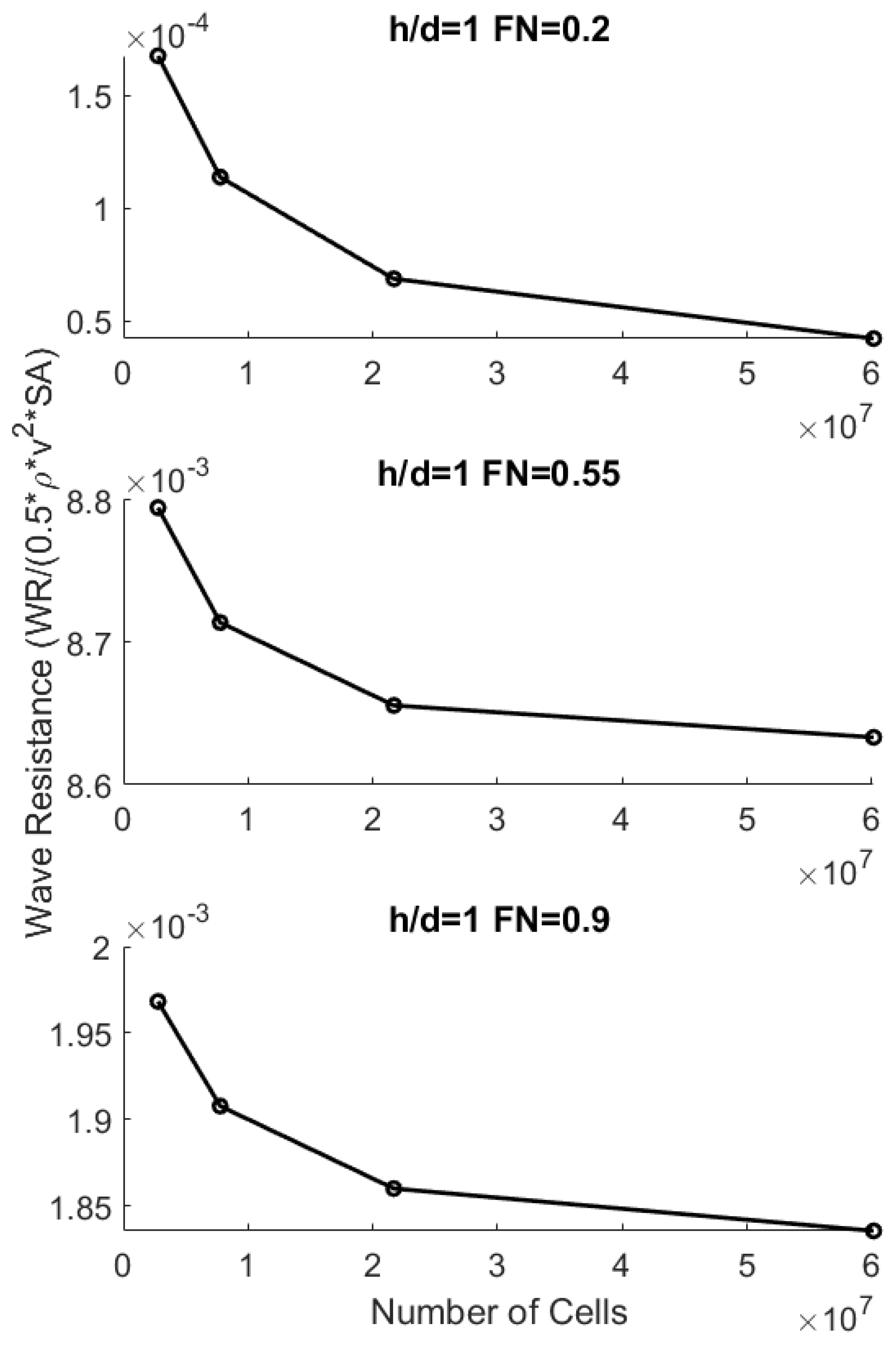
2.3. Simulation Validation

In addition to the above numerical sensitivity analysis, experimental validation of each simulation technique is also presented in order to ground results to a physical system. Using the meshing parameters determined in Section 2.1 and Section 2.2 for the BEM and CFD, respectively, steady-state near-surface simulations were conducted on an 8:1 prolate spheroid and compared to experiments performed by Weinblum in 1950 [25]. Experiments were performed on an 8:1 prolate spheroid with submergence $h/d=$ 1 in the Berlin tank, gathering total resistance values for Froude numbers between 0.2 and 0.4. The viscous portion of drag is subtracted from the total resistance for comparison to the present simulation techniques, which provide values of wave resistance. In this case, the viscous drag is composed of skin friction, which is estimated using the Schoenherr skin friction coefficient (also used by Weinblum) and a form drag correction given by the empirical formula of Hoerner in Equation (12) [26]. In this equation, $C_{\mathrm{Dform}}$ is the form drag coefficient based on the wetted area of the body, $C_f$ is the friction coefficient estimated by the Schoenherr friction line, and $d/l$ is the diameter-to-length ratio of the body.

$$\begin{array}{c}{C}_{\mathrm{Dform}}/C_f=1.5{(d/l)}^{\frac{3}{2}}+7{(d/l)}^3\end{array}$$

(12)

Figure 6 provides a comparison of the wave resistance predicted by the BEM and CFD simulations to the experimental values of Weinblum. Close experimental agreement for both simulation methods reveals that the simulation methods are capable of producing accurate wave-resistance values. Additionally, the CFD simulation predictions that make no simplifying free surface assumptions fall closer to the experimental results across all Froude numbers examined. This better agreement leads the authors to believe that the CFD method provides solutions closer to the ground truth. Finally, two viscous simulations are provided for the two highest forward velocities given in accordance with Section 3.4. The total resistance in these cases is reduced to the wave resistance in the same fashion as the experimental tests where skin friction and form drag are subtracted. The close agreement shows that viscous modeling is handled appropriately within this speed range.

3. Results and Discussion

In an effort to identify the effect of incorporating a linearized free-surface boundary condition in the prediction of near-surface steady-state wave making forces, several simulations of a shallowly submerged underwater vessel are completed using both the BEM and RANSE CFD solvers that are described in Section 2. A forward speed range of $FN=$ 0.2 to 0.9 is simulated while varying the depths of submergence from 0.51 to 4 diameters. Due to the higher computational speeds of the BEM, 31 different forward speeds are simulated at each submergence compared to 11 for CFD. The following results and analyses are broken into those parts that directly affect the operation of the craft, such as forces and moments, and those parts associated with the physical response of the system, for example the free-surface elevation and free-wave spectrum.

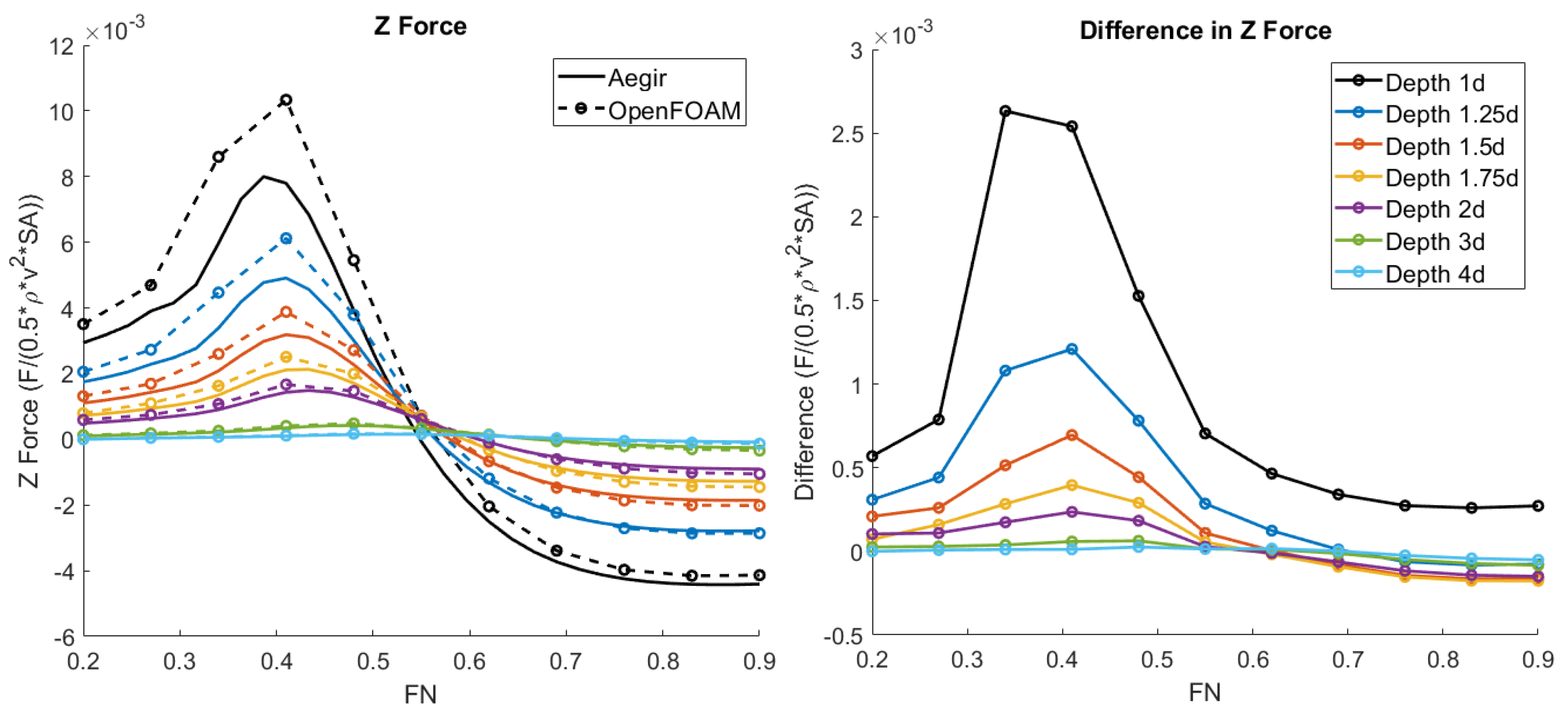
3.1. Forces and Moments

The forces and moments, which are calculated from pressure integration on the hull, impact the predicted motions of the vessel and directly inform parameter computations. Comparisons are shown in Figure 7, Figure 8 and Figure 9 of the predictions obtained using the BEM and RANSE CFD methods for the longitudinal force and moment acting on the body over a range of speeds and submergence depths. Additionally, each figure contains a plot of the difference (CFD minus BEM) between the simulation methods at each comparable data point.

The force along the x-axis is directly attributed to the wave-making resistance because neither model considers viscous forces. Figure 7 shows the normalized wave resistance versus the Froude number. The two methods produce qualitatively similar plots, which are maintained despite the depth of submergence. Very small resistance values are present for $FN<$ 0.35, at which point there is a rapid rise to a maximum between Froude numbers of 0.5 and 0.65 followed by a gradual decrease as the Froude number increases further. With respect to depth, the resistance values are greatest at small submergences and decrease to negligible values when deeply submerged. Additionally, the Froude number of greatest resistance shifts toward larger values with increasing depth. Focusing on the difference between the two simulation methods, RANSE CFD consistently produces values that are larger in magnitude than the BEM. The differences between the two methods, shown in the plots on the right sides of Figure 7, Figure 8 and Figure 9, show a similar structure to the force values themselves, showing that the differences between the two methods are governed by the wave making properties of the system. The disparities are greatest when wave making is strongest, revealing that one of the major error contributions could be due to the linearization of the free surface.

The structure of the normalized pitching moment with respect to the Froude number in Figure 8 is similar to the wave resistance. After negligibly small pitch moments at low Froude numbers, the moment increases to a maximum before gradually decreasing. As occurs for the resistance force, the forward speed at which the maximum moment is achieved shifts towards larger values as the depth increases. The difference between the two simulation methods shows that the largest differences occur when the moment is at a maximum, which occurs in a similar speed regime as the peak wave resistance. One anomaly to acknowledge is that the difference between the methods at a submergence of one diameter decreases at a faster rate than the other submergences.

Figure 9 shows the force acting on the vehicle in the vertical direction. This force plot has a different structure from the force along the x-axis and pitching moment. Even at small forward speeds, the vehicle has a small positive force towards the surface. This so-called suction force increases until a critical forward speed is reached, at which the vertical force switches to being a repulsive force away from the surface. This repulsive force increases in magnitude with increasing forward speeds until a nearly constant value is reached. The switch from suction to repulsion is known to occur physically, but the cause is unknown. A possible explanation is that at low speeds, the free surface acts similarly to a rigid surface, causing increased fluid velocities between the body and interface, increasing lift. However, at large speeds, the surface becomes deformed enough such that the wave pressure over the body overcomes the local suction force. Despite the overall different appearance of the vertical force, the RANSE CFD method results in more positive values over the submergence range and for Froude numbers less than 0.6.

Overall, for the forward speed and submergence range studied, there is a consistent difference between the force and moment predictions calculated using a BEM and RANSE CFD. These differences are largest for cases where the physical wave-making is strongest, which occurs for shallow submergences and within a critical forward speed range. One of the most significant differences between the two simulation methods is the direct application of a linearized free-surface boundary condition within the BEM. The assumptions that are tied to this linearization begin to fall apart in the cases of large wave-making, since the interface can no longer be assumed as a calm, undisturbed surface. The error incurred by adopting the linearized free-surface boundary condition may be significant if they are used to calculate parameters for a coefficient-based model. At their peaks, the two methods produce values that differ by 22.6%, 32.5%, and 33.3% for the x force, z force, and pitch moment, respectively.

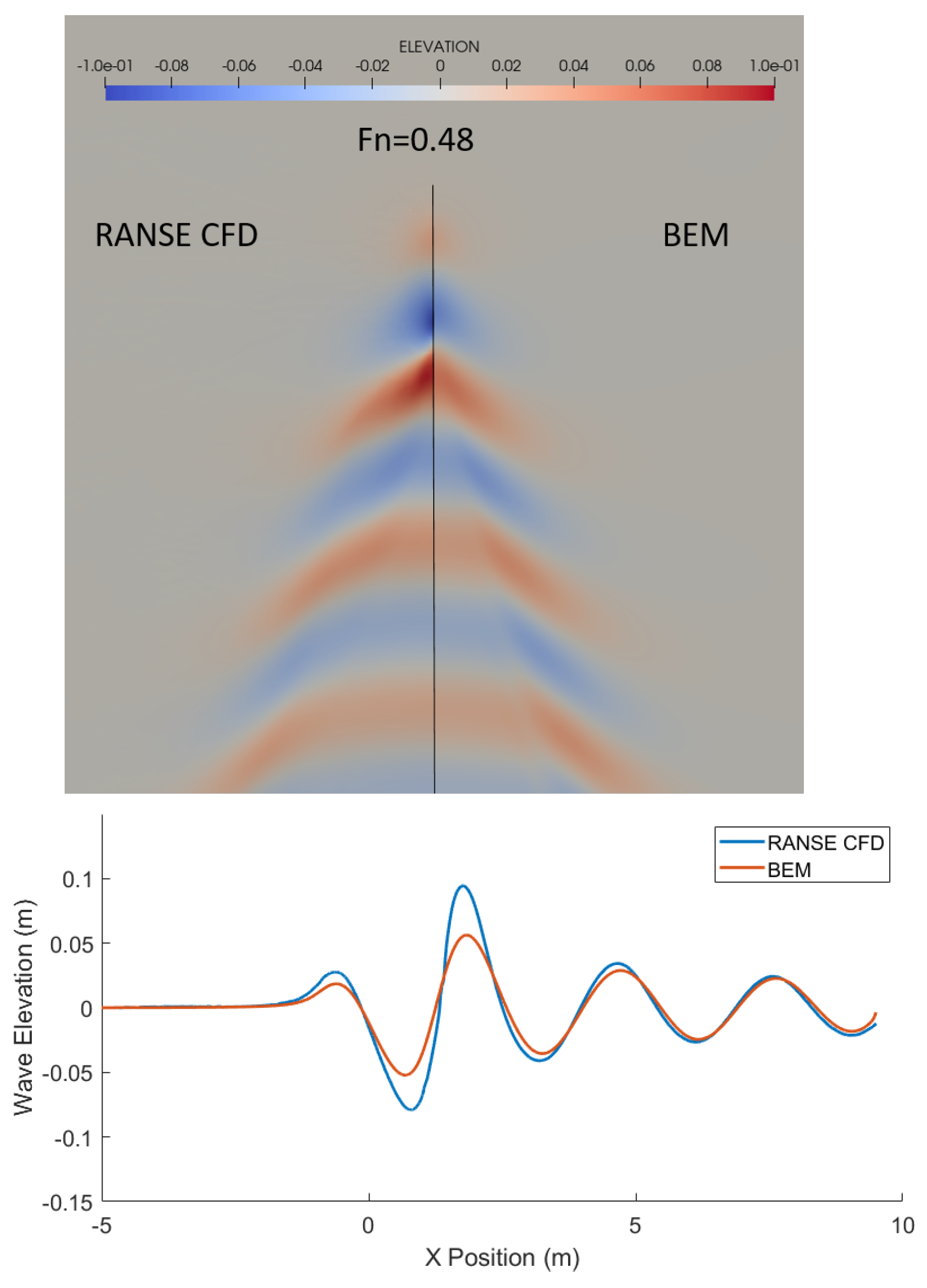
3.2. Wave Pattern and Longitudinal Wave Profile

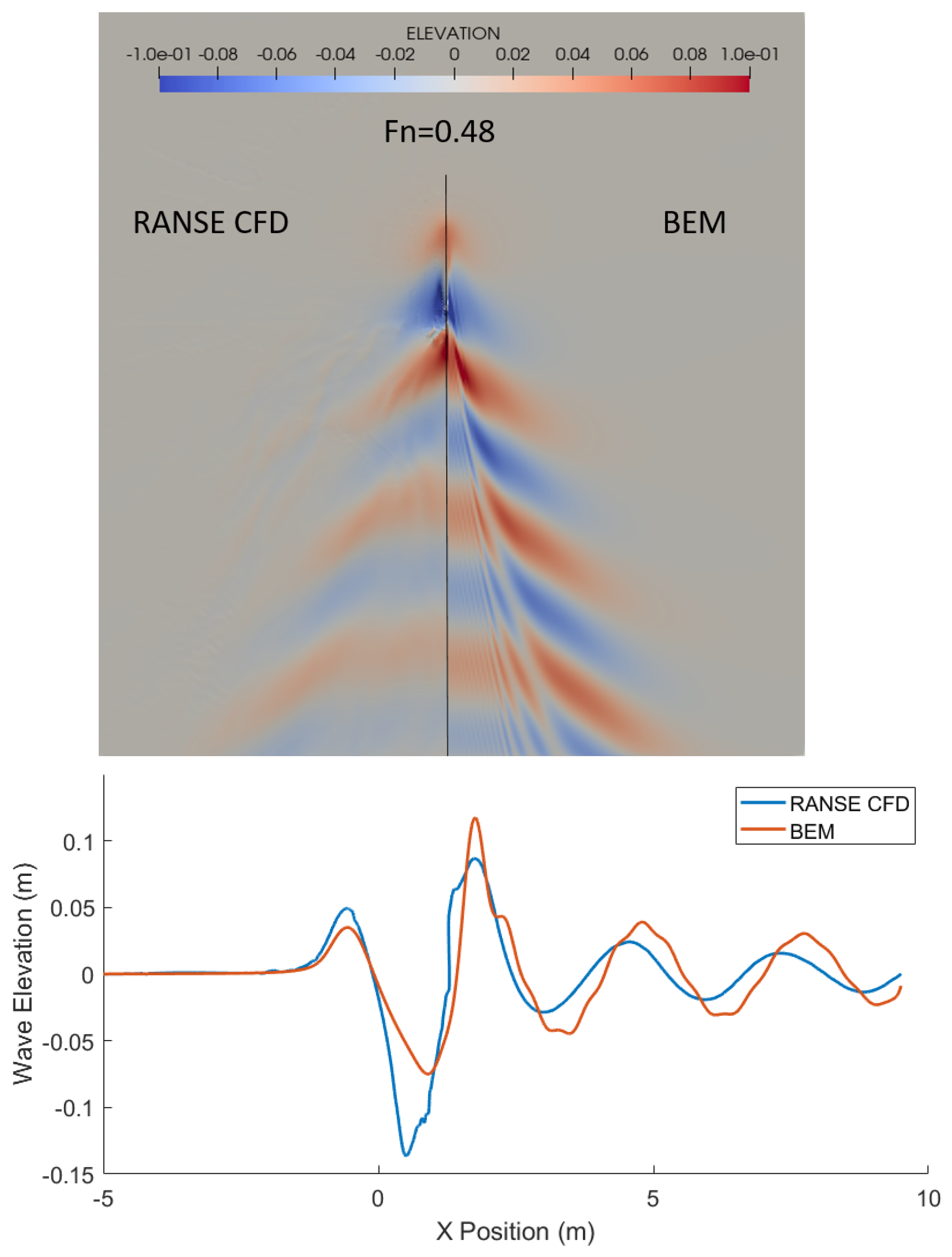
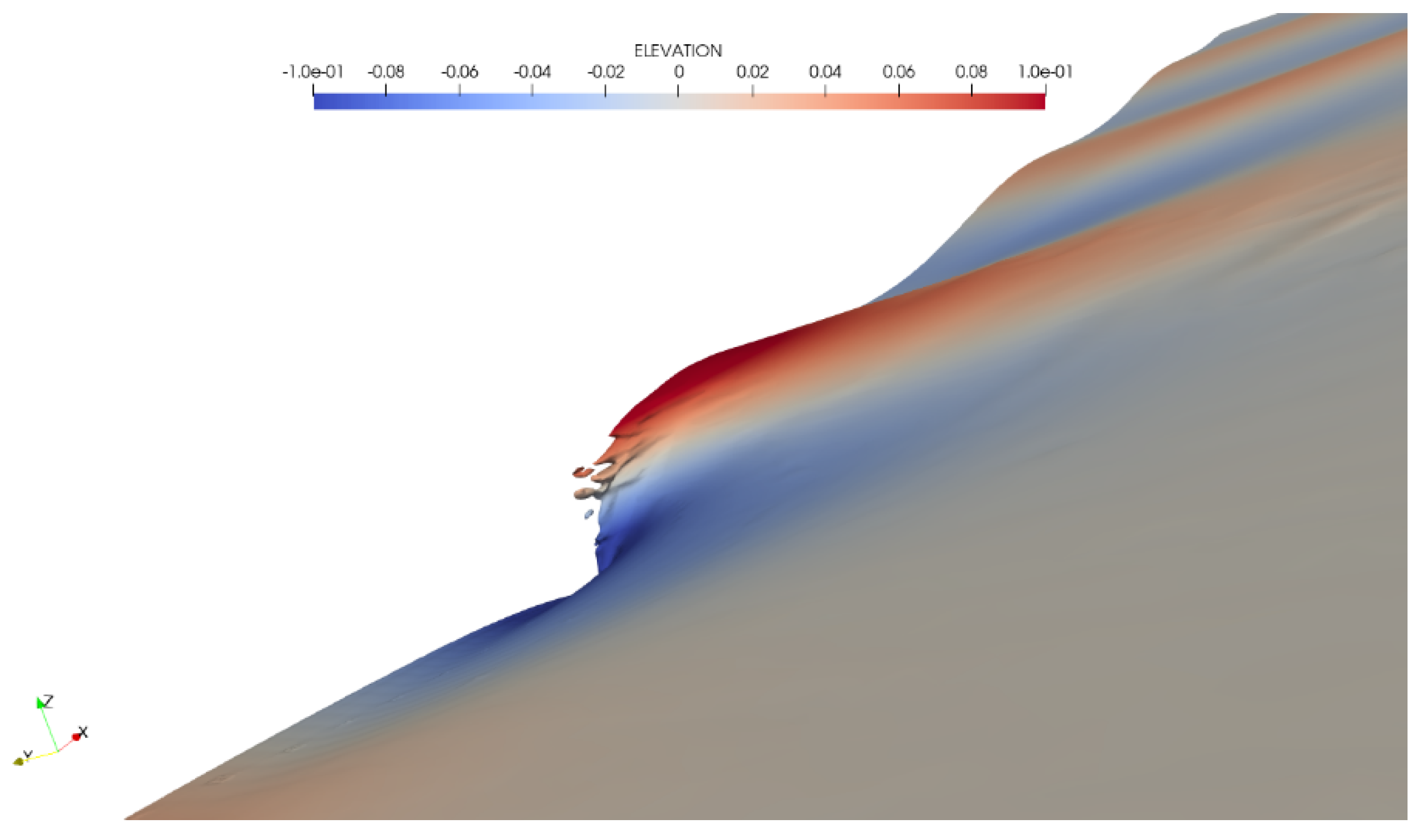
The differences that are observed in the hydrodynamic forces and moments between the BEM and RANSE CFD methods are the result of physical phenomena. The primary forcing mechanism in these cases is related to the creation of a steady-state wave train behind the vehicle. The creation of these waves alters the velocity and pressure field around the body and radiates energy away from the body. One can look to this wave field to find physical reasoning for the different force and moment predictions. Figure 10 and Figure 11 display renderings of the wave pattern for both the RANSE CFD (left) and BEM (right) methods for Froude numbers of 0.48 (Figure 10) and 0.69 (Figure 11) at a submergence of one diameter. Below each figure is a plot that shows the wave elevation along a longitudinal wave cut that is located one half diameter away from the central axis. Experimental wave elevation data for steady near-surface motions are largely unavailable, and therefore, comparisons are simply kept between the two simulation methods. The wave pattern differences are primarily attributed to the application of a simplifying free-surface boundary condition imposed within the BEM that is not imposed within the CFD simulations.

Initial observation shows how the wave patterns change with respect to the simulation parameter of forward speed. Increasing the forward speed of the vessel creates a longer primary wavelength along with more divergent waves that propagate orthogonal to the vehicle’s direction of motion. Secondly, one should acknowledge that although the speed is lower, the case of $FN=$ 0.48 corresponds to the larger wave resistance, which correlates to larger wave elevations. When larger waves are produced, there is more energy that is carried away from the system; thus, a simulation method that more accurately captures larger (and steeper) waves will be able to more accurately predict larger wave-making forces and moments.

Individually comparing the two simulation methods reveals some of the physical differences that contribute to the varying force and moment predictions. The BEM, with the linearized free surface boundary conditions, has decreased wave elevations and therefore smaller wave slopes. The RANSE CFD method, however, is able to realize larger waves without breaking any underlying assumptions. Being able to faithfully represent larger waves, especially close to the vessel, enables the RANSE CFD method to resolve larger wave-making forces explored in Section 3.1.

3.3. Breaking Waves

The ability of the RANSE CFD method to capture larger and steeper waves aids in its ability to predict forces and moments under a much larger range of operating conditions, including instances where nonlinear phenomena are present. For instance, wave breaking and overtopping occur when waves become too steep and fall over. The BEM, with its imposed linear free-surface boundary conditions, is not able to produce breaking waves. One can observe the effects of breaking waves on the force and moment predictions in Figure 12, Figure 13 and Figure 14, which show submergences of 1.25, 1, 0.75, and 0.51 diameters. The submergences of 1.25 and 1 diameter do not include instances of wave-breaking while the cases of 0.75 and 0.51 diameter do. In these cases, the predicted forces and moments behave differently from the other depths due to the presence of breaking waves. The presence of breaking waves results in much larger force and moment differences between the BEM and RANSE CFD solutions.

One can observe the physical presence and effects of breaking waves through the visual inspection of the wave pattern and free-surface elevations. The wave pattern and longitudinal wave cut of a spheroid traveling with $FN=$ 0.48 and submergence depth of 0.51 diameters are given in Figure 15. Close to the front of the wave pattern, near the vehicle location, much larger wave-elevation changes are present, signifying very steep waves. The presence of breaking waves is shown through a longitudinal wave cut at a distance of one half diameter from the center line. The wave profile for the CFD case becomes very steep and begins overtopping such that the profile can no longer be considered as a single-valued function. Looking further at the generated wave pattern, the BEM creates a much more coherent structure, particularly in the creation of a divergent wave train. An additional artifact that is observed is that the two simulation methods produce transverse wave patterns of slightly different wavelengths. Figure 16 gives a three-dimensional view of the breaking wave that is produced using RANSE CFD.

3.4. Viscous Effects

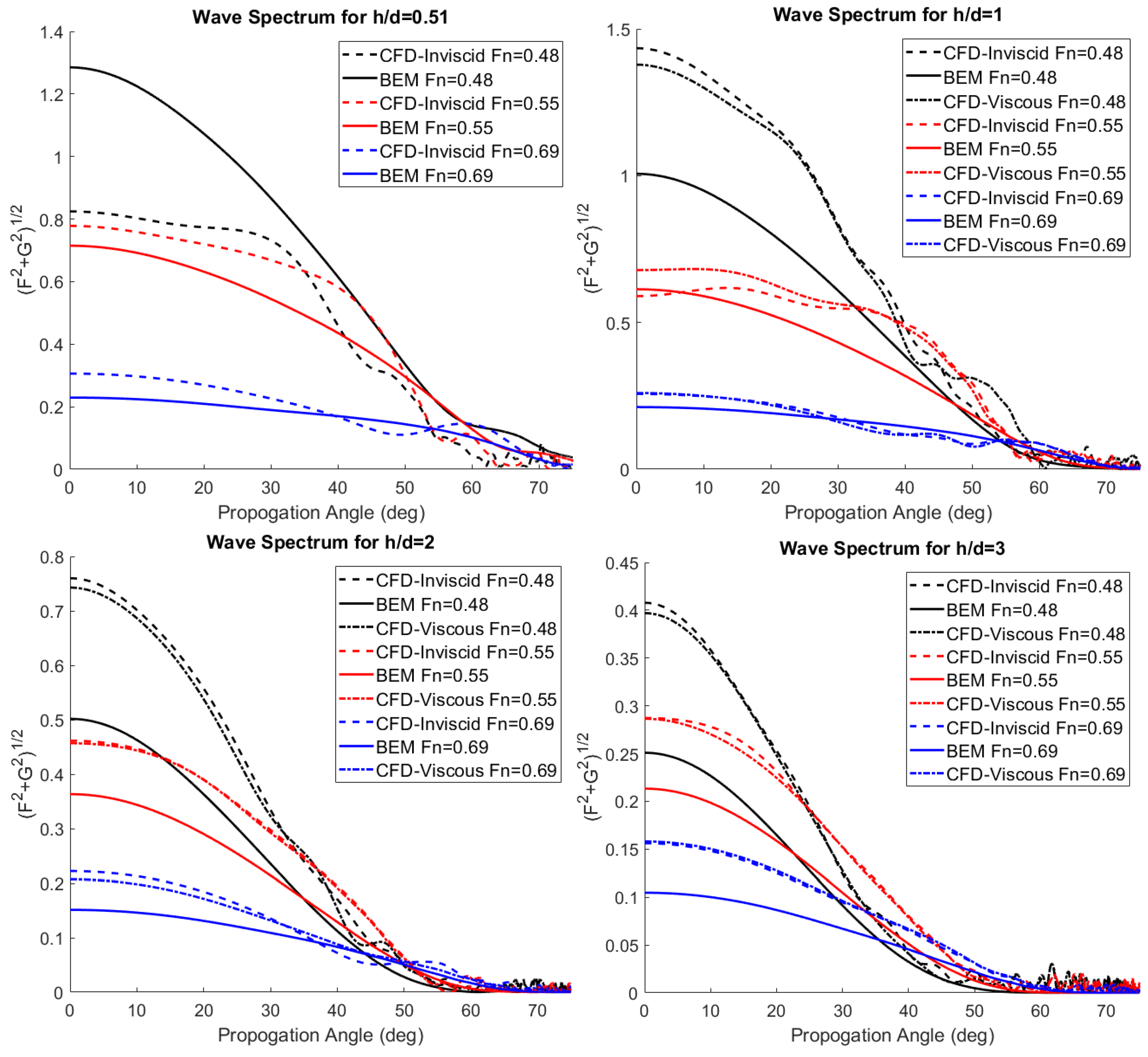
One shortcoming of the BEM and CFD methods used throughout this study is the application of potential flow and an inviscid fluid, respectively. Both methods, when applied to this point, neglect viscous effects such as skin friction and separated flow, which can contribute significantly to the hydrodynamic forces acting on a vehicle. Empirical methods are available using the forward speed and vehicle surface area to estimate the skin friction post hoc; however, these formulae do not depend on the depth of submergence. A brief study investigating the dependence on the depth of submergence for viscous forces is presented.

Viscous effects are included within the RANSE CFD simulation method by setting the fluid kinematic viscosity to a value of $1\times {10}^{-6}{\mathrm{m}}^2/\mathrm{s}$, defining a no-slip velocity condition on the body and applying the standard kOmegaSST turbulence model [27]. More sophisticated turbulence models are available that account for specific free-surface effects such as buoyancy [28]; however, the standard kOmegaSST model is sufficient in modeling the relatively simple, unbroken free surface. Wall functions are used to model the boundary layer around the body so that a similarly refined mesh can be used for both the inviscid and viscous cases. A small number of prism layers were added to guarantee consistent cell sizing around the body; however, the kOmegaSST turbulence model is said to be insensitive to changes in the y+, a parameter used to describe the cell thickness next to a body. This fact is confirmed by simulating a spheroid, with varied y+ values, at a submergence depth of one diameter and $FN=$ 0.55. Three meshes were simulated, where the average y+ values were 236.7, 90.1, and 28.3. The resulting force values were 65.6, 65.2, and 65.9 N, corresponding to a maximum percent difference of 1.1% with respect to the simulation using the lowest y+. An example of the meshes including prism layers is given in Figure 17. The large y+ case, which corresponds to the same mesh used in the inviscid simulations, was chosen due to its lower computational cost.

Steady-state simulations of a shallowly submerged prolate spheroid traveling with Froude numbers of 0.34, 0.48, 0.55, and 0.69 is simulated in a viscous and inviscid fluid using the RANSE CFD solver OpenFOAM. These forward speeds result in Reynolds numbers ranging from 3 million to 6.1 million, which is largely turbulent flow, and thus the standard kOmegaSST turbulence model was deemed appropriate. Understanding the shortcomings of attempting to fully capture transient wave-breaking discussed in Section 3.3, submergence depths of 1–4 diameters were prescribed so that wave breaking would not be present. Figure 18 compares the forces in the x-direction with respect to depth of submergence for each forward velocity. The figure contains an additional plot demonstrating how the difference between the viscous and inviscid cases changes with respect to submergence.

As the body approaches a deeply submerged condition, the force acting along the x-axis of the body decays asymptotically to a constant value despite the forward speed. The viscous cases decay to a positive nonzero value, while the inviscid cases approach zero. The quadratic dependence on forward velocity is captured within the normalization process. The difference between the viscous and inviscid cases represents the additional force acting on the body due to viscous phenomena such as skin friction and form drag. The difference is not constant-valued with respect to depth meaning that viscous forces are dependent on the body’s proximity to the free surface.

The depth dependence of viscous forces is elucidated by observing the fluid velocity contours around the body. Figure 19 shows the velocity magnitude contours around the spheroid operating with $FN=$ 0.55 and submergence depths of 4, 1.75, 1.25, and 1 diameters. The velocity contours show the separated wake behind the body. When the body is far away from the surface, the separated wake (shown in blue) extends directly behind the aft of the vessel. As the body approaches the surface, the separated wake moves towards the top of the vessel and begins to follow the contour of the disturbed free surface. The movement of the wake in this manner changes the dynamic pressure acting on the body, thus changing the hydrodynamic forces. This depth dependence would make the post hoc inclusion of viscous forces using empirical methods more involved.

3.5. Wave Spectrum

Visually, there is evidence that the RANSE CFD produces larger wave elevations yielding higher wave-making forces on the body. A wave spectrum analysis is carried out to quantify the energy content within the wave train. A transverse wave cut method [29] is applied to estimate the wave-making characteristics in each simulated case using the longitudinal wave slope along a perpendicular slice to the wave pattern located 0.6 body lengths (1.2 m) behind the stern. The transverse wave cut method has previously been used to identify nonlinearities in the wave patterns produced by the linear and nonlinear versions of the boundary element method used throughout this study [14]. This method has also been successfully applied to characterize the wave-making properties of high speed craft [30] and validated against other wave-cut methods [31].

The process outlined by Eggers [29] begins by taking the Fourier transform of both the wave elevation, $\zeta$ (Equation (13)), and longitudinal wave slope, ${\zeta }_x$ (Equation (14)), along a transverse cut of the wave pattern. In these equations U and S represent the real and imaginary parts of the Fourier transform, while the subscript x corresponds to the values derived from the wave slope. The value u represents the circular wave number in the transverse direction. The even (subscript e) and odd (subscript o) parts of the sine (F) and cosine (G) components of the free-wave spectrum are given in Equations (15) and (16). The arbitrary function $s(u)$ is given in Equation (17). Furthermore, we can relate the independent circular transverse wave number, u, to the wave propagation angle, $\theta$, through Equation (18). The wave propagation angle helps identify the primary direction of wave motion. For example, longitudinal waves move parallel to vehicle velocity while divergent waves propagate orthogonal to vehicle velocity.

$$\begin{array}{cc}\hfill C(u,x)+iS(u,x)={\int }_{-\infty }^{\infty }\zeta (x,y)\exp (iuy)dy& \\ \hfill 0\le u<\infty \end{array}$$

(13)

$$\begin{array}{cc}\hfill C_x(u,x)+i{S}_x(u,x)={\int }_{-\infty }^{\infty }{\zeta }_x(x,y)\exp (iuy)dy& \\ \hfill 0\le u<\infty \end{array}$$

(14)

$$\begin{array}{cc}\hfill i{F}_e(u)+G_e(u)=& 2\{sC(u,x)\exp (isx)\hfill \\ & +i{C}_x(u,x)\exp (isx)\}/s\hfill \end{array}$$

(15)

$$\begin{array}{cc}\hfill F_o(u)-i{G}_o(u)=& 2\{sS(u,x)\exp (isx)\hfill \\ & +i{S}_x(u,x)\exp (isx)\}/s\hfill \end{array}$$

(16)

$$\begin{array}{c}\hfill s(u)={\{(1+\sqrt{1+4u^2})/2\}}^{1/2}>0\end{array}$$

(17)

$$\begin{array}{c}\hfill u=sec(\theta )tan(\theta )\end{array}$$

(18)

The total amplitude of the free-wave spectrum (${(F^2+G^2)}^{1/2}$) corresponds to the energy content within waves propagating at a particular angle, $\theta$. Figure 20 shows the wave spectra for simulations of $h/d=$ 0.51, 1, 2, and 3. Note that viscous results at $h/d=$ 0.51 are absent due to difficulty in turbulence modeling for wave-breaking cases. Some general trends that are immediately evident between the spectra are that the energy content is greatest for waves traveling at small propagation angles (transverse waves) and that the relative magnitude of the energy content decreases with increasing depth of submergence. Additionally, the spectra of greatest magnitude are in general the cases of $FN=$ 0.48, which also produce larger wave resistance values. Note that the wave resistance is an integral of the free-wave spectrum.

Comparing the individual cases, the wave spectra for submergences where wave breaking is not present ($h/d\ge 1$) are similarly structured with respect to propagation angle. The spectra produced using RANSE CFD generally result in larger magnitude values than the BEM. As seen in Section 3.2, this is the result of the production of larger wave elevations containing more energy. Because the BEM does not capture wave breaking, the spectrum magnitudes produced by the BEM continue increasing in cases of small submergence and peak forward speeds even surpassing the CFD results. Energy is lost through the process of wave breaking, creating less coherent wave structures, as seen in Section 3.3, while dissipating energy away from the system in other manners. The ability of a simulation method to capture the energy content in a wave system is dependent on the generation of an accurate wave pattern. The application of linearized boundary conditions, which decrease wave elevations, shows lower energy content than simulation methods that make no such assumptions on the surface.

Furthermore, we compare the difference between the free-wave spectra that are produced when viscosity is introduced to the system. The relative difference between the viscous and inviscid spectra, barring results from the wave-breaking cases, is small compared to the difference between CFD and the BEM. The difference also remains fairly constant with respect to depth. This is in contrast with the results presented in Section 3.4, which showed a depth dependence on the force. The difference between these results shows that the inclusion of viscosity does not significantly alter the wave pattern, but rather, the additional depth-dependent forces are attributed to skin friction and the creation/movement of a separated wake.

4. Conclusions

The accurate prediction of hydrodynamic forces is necessary for the development of a Lagrangian maneuvering and seakeeping model for underwater vehicles traveling close to a freely deformable surface. A boundary element method using a linearized free surface has been used previously for state-dependent parameter estimations to populate the coefficient-based model; however, the assumptions behind the linear free surface break down at large speeds and small submergences, when wave generation is large. The errors associated with making these kinds of assumptions are well understood for surface-piercing bodies; however, further efforts are needed to better characterize the effects for shallowly submerged underwater vehicles of variable depth that do not break the calm water surface. This study compares the hydrodynamic response of a steadily traveling prolate spheroid near the surface that is simulated using two different methods.

Simulating a free surface using an interface capturing RANSE CFD model that makes no direct linearization and suppresses the effect of viscosity to allow a clearer comparison with the BEM, the forces in the x and z directions are 22.6% and 32.5% larger, respectively, compared to a BEM that incorporates linearized free surface boundary conditions. The pitch moment of the CFD method shows values 33.3% larger than the BEM. Another interesting observation is that the z force switches directions from suction to a repulsive force as the body approaches the free surface and increases in forward velocity. Wave elevations due to the body’s motion are almost 50% larger in the CFD simulations when compared to the BEM. The wave elevation increase is expected and corresponds to similar increases in the force and moments. The difference in the force and moment predictions between the two methods appears to follow the same trends as the observed values. This supports the idea that the differences are due to the inclusion of linearized free surface boundary conditions as the largest differences occur when the body is shallowly submerged and generating large free-surface deformations.

Including viscosity in the CFD simulations shows that a depth-independent viscous correction is not valid in the case of a shallowly submerged vehicle. The force acting in the x-direction is not constant with depth. A possible explanation is the creation of a separated wake with a separation point that drifts toward the top of the vehicle as submergence depth decreases. Although the additional viscous forces are not constant with depth, a free-wave spectrum analysis showed that viscosity does not have a large effect on the creation of the steady state wave train behind the body.

Future efforts, using the results of this study, are aimed at the calculation of the LNMS model parameters. Parameter computation methods will be focused on methods that can accurately capture the free surface without making linearization assumptions on the boundaries. Impulsive motion simulations using OpenFOAM are currently being explored. Additionally, effort is focused on finding better free surface refinement techniques to more accurately capture small free-surface deformations.

References

1. Battista, T. Lagrangian Mechanics Modeling of Free Surface-Affected Marine Craft. Ph.D. Thesis, Virginia Tech, Blacksburg, VA, USA, 2018. [Google Scholar]
2. Valentinis, F.; Battista, T.; Woolsey, C. A Maneuvering Model for an Underwater Vehicle Near a Free Surface—Part III: Simulation and Control Under Waves. IEEE J. Ocean. Eng. 2023, 1–26. [Google Scholar] [CrossRef]
3. Valentinis, F.; Donaire, A.; Perez, T. Energy-Based Motion Control of a Slender Hull Unmanned Underwater Vehicle. Ocean Eng. 2015, 104, 604–616. [Google Scholar] [CrossRef]
4. Woolsey, C.A.; Techy, L. Cross-Track Control of a Slender, Underactuated AUV Using Potential Shaping. Ocean Eng. 2009, 36, 82–91. [Google Scholar] [CrossRef]
5. Battista, T.; Valentinis, F.; Woolsey, C. A Maneuvering Model for an Underwater Vehicle Near a Free Surface—Part I: Motion Without Memory Effects. IEEE J. Ocean. Eng. 2020, 45, 212–226. [Google Scholar] [CrossRef]
6. Battista, T.; Valentinis, F.; Woolsey, C. A Maneuvering Model for an Underwater Vehicle Near a Free Surface—Part II: Incorporation of the Free Surface Memory. IEEE J. Ocean. Eng. 2023, 1–12. [Google Scholar] [CrossRef]
7. Jung, S.; Brizzolara, S.; Woolsey, C. An Approach for Computing Parameters for a Lagrangian Nonlinear Maneuvering and Seakeeping Model of Submerged Vessel Motion. IEEE J. Ocean. Eng. 2021, 46, 749–764. [Google Scholar] [CrossRef]
8. Jung, S.; Brizzolara, S.; Woolsey, C.A. Parameter Computation for a Lagrangian Mechanical System Model of a Submerged Vessel Moving near a Free Surface. Ocean Eng. 2021, 230, 108988. [Google Scholar] [CrossRef]
9. Raven, H.C. A Solution Method for the Nonlinear Wave Resistance Problem. Ph.D. Thesis, Delft University of Technology, Delft, NL, USA, 1996. [Google Scholar]
10. White, P.F.; Piro, D.J.; Knight, B.G.; Maki, K.J. A Hybrid Numerical Framework for Simulation of Ships Maneuvering in Waves. J. Ship Res. 2022, 66, 159–171. [Google Scholar] [CrossRef]
11. Abdul Khader, M.H. Effects of Wave Drag on Submerged Bodies. La Houille Blanche, 1979; pp. 465–470. Available online: https://www.shf-lhb.org/articles/lhb/pdf/1979/05/lhb1979044.pdf (accessed on 1 April 2023).
12. Chey, Y.H. The Consistent Second-Order Wave Theory and Its Application to a Submerged Spheroid. J. Ship Res. 1970, 14, 23–50. [Google Scholar] [CrossRef]
13. Tuck, E.; Scullen, D. A Comparison of Linear and Nonlinear Computations of Waves Made by Slender Submerged Bodies. J. Eng. Math. 2002, 42, 255–264. [Google Scholar] [CrossRef]
14. Lambert, W.; Brizzolara, S. On the Effect of Non-Linear Boundary Conditions on the Wave Disturbance and Hydrodynamic Forces of Underwater Vehicles Travelling Near the Free-Surface. In Proceedings of the ASME 2020 39th International Conference on Ocean, Offshore and Arctic Engineering, Online, 3–7 August 2020; American Society of Mechanical Engineers Digital Collection: New York, NY, USA, 2020. [Google Scholar]
15. Lambert, W.; Brizzolara, S.; Woolsey, C. On the Effect of Free-Surface Linearization on the Predicted Hydrodynamic Response of Underwater Vehicles Travelling Near the Free-Surface. In Proceedings of the OMAE 2022, Hamburg, Germany, 5–11 June 2022. [Google Scholar]
16. Kring, D.C.D.C. Time Domain Ship Motions by a Three-Dimensional Rankine Panel Method. Ph.D. Thesis, Massachusetts Institute of Technology, Cambridge, MA, USA, 1994. [Google Scholar]
17. Lambert, W.B.; Brizzolara, S. Wave Resistance Reduction for Ships Traveling in Fleet Formation. In Proceedings of the SNAME Maritime Convention, Virtual, 29 September 2020. [Google Scholar]
18. Rosenthal, B.; Datla, R.; Greeley, D.; Kring, D.; Keipper, T.; Milewski, B. Optimization Validation of a High-Speed Boat. In Proceedings of the 2013 Summer Computer Simulation Conference (SCSC’13), Toronto, ON, Canada, 7–10 July 2013; Society for Modeling & Simulation International: Vista, CA, USA, 2013; pp. 1–8. [Google Scholar]
19. Gouveia, R.; Fitzpatrick, S.; Costa, A.; Kring, D. Time Domain Simulation of Lifting Bodies Acting at or Near the Free Surface With Vortex Particle Wakes. J. Fluids Eng. 2019, 141, 041201. [Google Scholar] [CrossRef]
20. Brizzolara, S. Automatic Optimisation of a New Fast Catamaran with Bulbous Bow. In Proceedings of the International Conference on High-Performance Marine Vehicles (HIPER 2004), Rome, Italy, 27–29 September 2004; pp. 116–128. [Google Scholar]
21. Brizzolara, S.; Vernengo, G.; Bonfiglio, L.; Bruzzone, D. Comparative Performance of Optimum High Speed SWATH and Semi-SWATH in Calm Water and in Waves. In Proceedings of the SNAME Maritime Convention and 5th World Maritime Technology Conference, Providence, RI, USA, 3–7 November 2015. [Google Scholar]
22. Doyle, W.J.; Schambach, L.S.; Smith, M.V.; Field, C.; Hart, C.J. Verification, Validation, and Best Practices for a High-Order, Potential-Flow Boundary Element Method. In Proceedings of the SNAME 13th International Conference on Fast Sea Transportation, Washington, DC, USA, 1–4 September 2015. [Google Scholar]
23. Weller, H.; Tabor, G.; Jasak, H.; Fureby, C. A Tensorial Approach to Computational Continuum Mechanics Using Object Orientated Techniques. Comput. Phys. 1998, 12, 620–631. [Google Scholar] [CrossRef]
24. Lyu, W.; el Moctar, O. Numerical and Experimental Investigations of Wave-Induced Second Order Hydrodynamic Loads. Ocean Eng. 2017, 131, 197–212. [Google Scholar] [CrossRef]
25. Weinblum, G.; Amtsberg, H.; Bock, W. Tests on Wave Resistance of Immersed Bodies of Revolution; Technical Report; Defense Technical Information Center: Potomac, VA, USA, 1950. [Google Scholar]
26. Hoerner, S.F. Fluid Dynamic Drag: Practical Information on Aerodynamic Drag and Hydrodynamic Resistance, 2nd ed.; Hoerner Fluid Dynamics: Bakersfield, CA, USA, 1965; Chapter 6C. [Google Scholar]
27. Menter, F.; Kuntz, M.; Langtry, R. Ten years of industrial experience with the SST turbulence model. Heat Mass Transf. 2003, 4, 625–632. [Google Scholar]
28. Devolder, B.; Troch, P.; Rauwoens, P. Performance of a buoyancy-modified k-ω and k-ω SST turbulence model for simulating wave breaking under regular waves using OpenFOAM. Coast. Eng. 2018, 138, 49–65. [Google Scholar] [CrossRef]
29. Eggers, K.W.H. An Assessment of Some Experimental Methods for Determining the Wavemaking Characteristics of a Ship Form. Trans. SNAME 1967, 75, 112–157. [Google Scholar]
30. Brizzolara, S.; Bruzzone, D.; Cassella, P.; Scamardella, I.; Zotti, I. Wave Resistance and Wave Patterns for High-Speed Crafts; Validation of Numerical Results by Model Test. In Proceedings of the 22nd Symposium on Naval Hydrodynamics, Washington, DC, USA, 9–14 August 1998; pp. 69–83. [Google Scholar]
31. Janson, C.E.; Spinney, D. A Comparison of Four Wave Cut Analysis Methods for Wave Resistance Prediction. Ship Technol. Res. 2004, 51, 173–184. [Google Scholar] [CrossRef]
Figure 1. A 2D visualization of the prolate spheroid and submergence depths used in simulations. Submergence depths are measured from the body axis of symmetry to the calm-water surface and given as a factor of the body diameter.
Jmse 11 00981 g001
Figure 2. Domain extent sensitivity analysis for three different Froude numbers (reported on top of each graph) and a submergence depth of one diameter.
Jmse 11 00981 g002
Figure 3. Mesh density sensitivity analysis for three different Froude numbers (reported on top of each graph). An increasing mesh multiple represents a smaller panel size.
Jmse 11 00981 g003
Figure 4. Mesh sensitivity analysis for 3D RANSE simulations using OpenFOAM.
Jmse 11 00981 g004
Figure 5. A representation of the free surface and body discretization used in the BEM (left) and CFD (right) simulations.
Jmse 11 00981 g005
Figure 6. Correspondence of BEM and CFD simulation data to experimental wave resistance values for an 8:1 prolate spheroid that is submerged 1 diameter from the surface. Small differences show that both the BEM and CFD simulations are capable of predicting accurate wave-resistance values with the CFD simulation performing marginally better.
Jmse 11 00981 g006
Figure 7. x force vs. Froude number at several test submergences. The left plot shows the value of normalized force for both the BEM (solid) and RANSE CFD (dotted) simulations. The right plot shows the difference (CFD minus BEM) between the simulations.
Jmse 11 00981 g007
Figure 8. Pitch moment vs. Froude number at several test submergences. The left plot shows the normalized moment value for both the BEM (solid) and RANSE CFD (dotted) simulations. The right plot shows the difference (CFD minus BEM) between the simulations.
Jmse 11 00981 g008
Figure 9. z force vs. Froude number at several test submergences. The left plot shows the value of normalized force for both the BEM (solid) and RANSE CFD (dotted) simulations. The right plot shows the difference (CFD minus BEM) between the simulations.
Jmse 11 00981 g009
Figure 10. Wave pattern and longitudinal wave cut for a spheroid traveling with a submergence of one diameter and a Froude number of 0.48.
Jmse 11 00981 g010
Figure 11. Wave pattern and longitudinal wave cut for a spheroid traveling with a submergence of one diameter and a Froude number of 0.69.
Jmse 11 00981 g011
Figure 12. x force vs. Froude number at several test submergences at which wave breaking occurs. The left plot shows the value of normalized force for both the BEM (solid) and RANSE CFD (dotted) simulations. The right plot shows the difference (CFD minus BEM) between the simulations.
Jmse 11 00981 g012
Figure 13. Pitch moment vs. Froude number at several test submergences at which wave breaking occurs. The left plot shows the normailzed moment value for both the BEM (solid) and RANSE CFD (dotted) simulations. The right plot shows the difference (CFD minus BEM) between the simulations.
Jmse 11 00981 g013
Figure 14. z force vs. Froude number at several test submergences at which wave breaking occurs. The left plot shows the value of normalized force for both the BEM (solid) and RANSE CFD (dotted) simulations. The right plot shows the difference (CFD minus BEM) between the simulations.
Jmse 11 00981 g014
Figure 15. Wave pattern and longitudinal wave cut for a spheroid travelling with a submergence of 0.51 diameters and a Froude number of 0.48.
Jmse 11 00981 g015
Figure 16. Zoomed-in view of a breaking wave on top of a spheroid travelling with a submergence of 0.75 diameters and a Froude number of 0.48.
Jmse 11 00981 g016
Figure 17. A zoomed-in view of the simulation mesh around the aft portion of a prolate spheroid. The meshes contain different numbers of prism layers to achieve the displayed y+ value and help create a consistent boundary layer.
Jmse 11 00981 g017
Figure 18. Force in the x direction vs. depth of submergence for 4 different forward velocities using viscous and inviscid RANSE CFD. The left plot shows the value of normalized force for both simulations. The right plot shows the difference (viscous minus inviscid) between the simulations.
Jmse 11 00981 g018
Figure 19. Velocity magnitude contours around a shallowly submerged prolate spheroid in a viscous fluid. The separated wake (shown in blue) moves toward the surface as the body submergence decreases.
Jmse 11 00981 g019
Figure 20. Free-wave spectrum data calculated using a transverse wave cut method for depths of submergence of 0.51, 1, 2, and 3 diameters.
Jmse 11 00981 g020
Disclaimer/Publisher’s Note: The statements, opinions and data contained in all publications are solely those of the individual author(s) and contributor(s) and not of MDPI and/or the editor(s). MDPI and/or the editor(s) disclaim responsibility for any injury to people or property resulting from any ideas, methods, instructions or products referred to in the content.