
Reconstructing Long-Term Arctic Sea Ice Freeboard, Thickness, and Volume Changes from Envisat, CryoSat-2, and ICESat-2


 ,
,
Abstract
Simple Summary
Abstract
1. Introduction
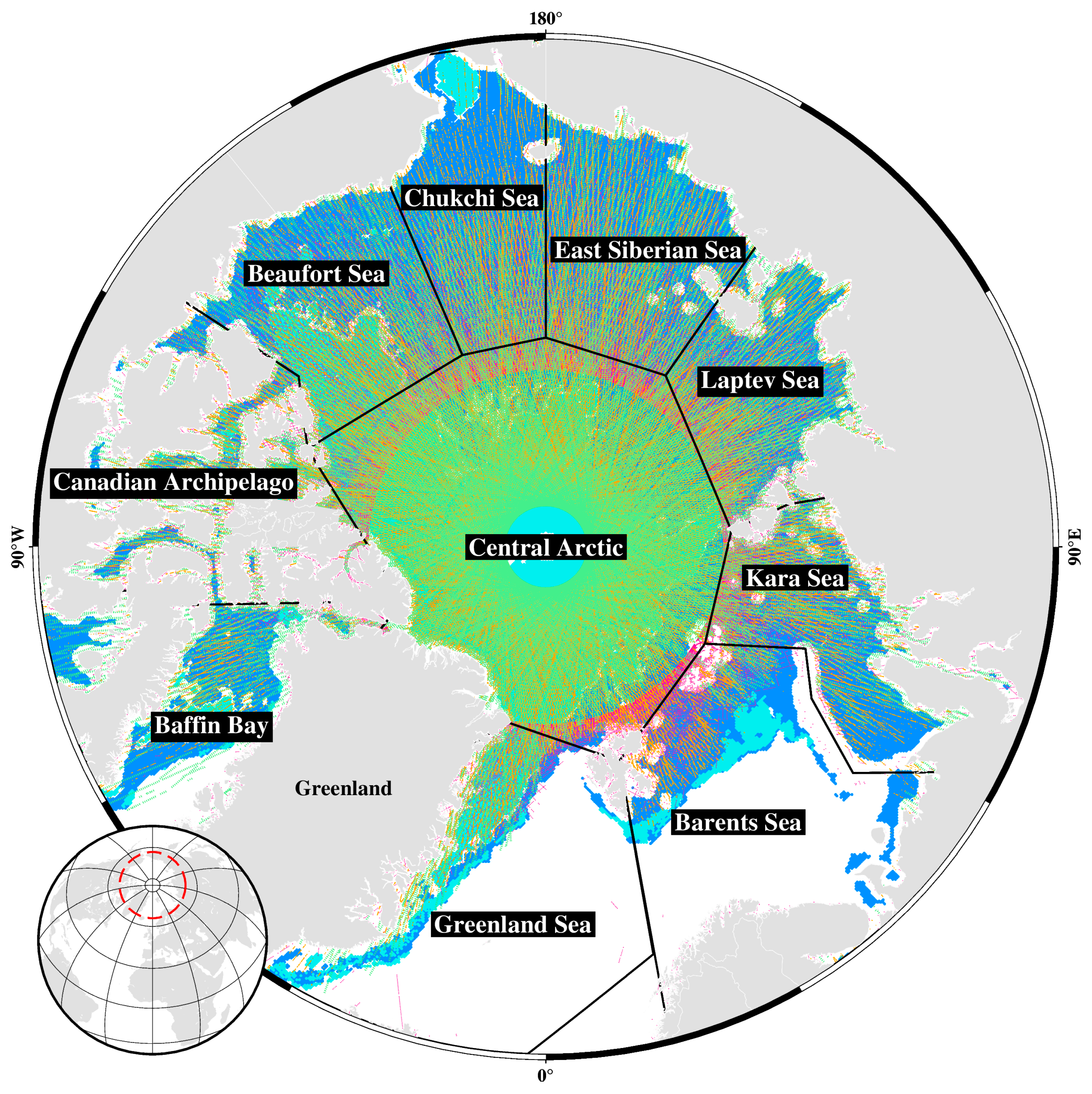
2. Study Area
3. Data
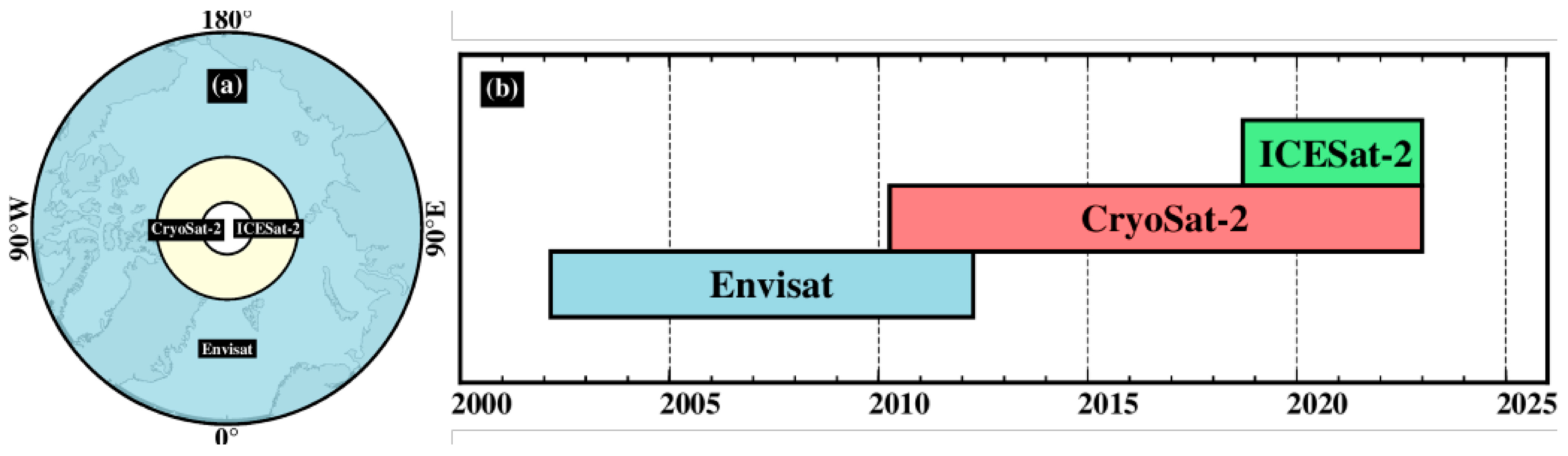
3.1. Satellite Altimetry Data and Mean Sea Surface (MSS) Model
3.1.1. Envisat Data
3.1.2. CryoSat-2 Data
3.1.3. ICESat-2 Data
3.1.4. MSS Model


| Data Types | Data Source | Spatial Resolution | Period | Coverage | Orbit Inclination | Reference Ellipsoid | Used | ||
|---|---|---|---|---|---|---|---|---|---|
| Spatial | Time | ||||||||
| Satellite Altimetry | Envisat | ESA (GDR) | — | 35 d | 2002–2010 | 81.5° S–81.5° N | 98.5° | WGS84 | Freeboard retrieval |
| CryoSat-2 | ESA (GDR) | — | 30 d | 2010-present | 88° S–88° N | 92° | WGS84 | Freeboard retrieval | |
| ICESat-2 | NASA | — | 91 d | 2018-present | 88° S–88° N | 92° | WGS84 | Freeboard retrieval | |
| Mean Sea Surface Height | CLS01 | Envisat | 2′ × 2′ | — | 1993–1999 | 80° S–82° N | — | Topex/Poseidon | Freeboard retrieval |
| DTU15 | DTU | 1′ × 1′ | — | 1991–2015 | 90° S–90° N | — | Topex/Poseidon | Freeboard retrieval | |
| DTU18 | DTU | 1′ × 1′ | — | 1993–2017 | 90° S–90° N | — | Topex/Poseidon | Freeboard retrieval | |
| DTU21 | DTU | 1′ × 1′ | — | 1993–2020 | 90° S–90° N | — | Topex/Poseidon | Freeboard retrieval | |
| Ancillary Data | Sea ice type | OSI SAF | 10 km | Daily | 2005/03-present | Arctic/Antarctic | — | — | Thickness retrieval |
| Snow depth | NASA | 100 km | Daily | 2000–2015 | Arctic | — | — | Thickness retrieval | |
| Snow density | NASA | 100 km | Daily | 2000–2015 | Arctic | — | — | Thickness retrieval | |
| Sea ice density | Alexandrov (2010) | MYI: 882.0 kg/m3 FYI: 916.7 kg/m3 | Thickness retrieval | ||||||
| Sea water density | Alexandrov (2010) | Fixed value: 1024 kg/m3 | Thickness retrieval | ||||||
| Sea ice area | NSIDC | — | Monthly | 1978-present | Arctic | — | — | Volume retrieval | |
| Sea surface temperature | NOAA | 25 km | Daily | 1981-present | 90° S–90° N | — | — | Impact factors | |
| Sea surface wind filed | NOAA | varying | Monthly | 1948-present | 90° S–90° N | — | — | Impact factors | |
3.2. Validation Data
3.3. Ancillary Data
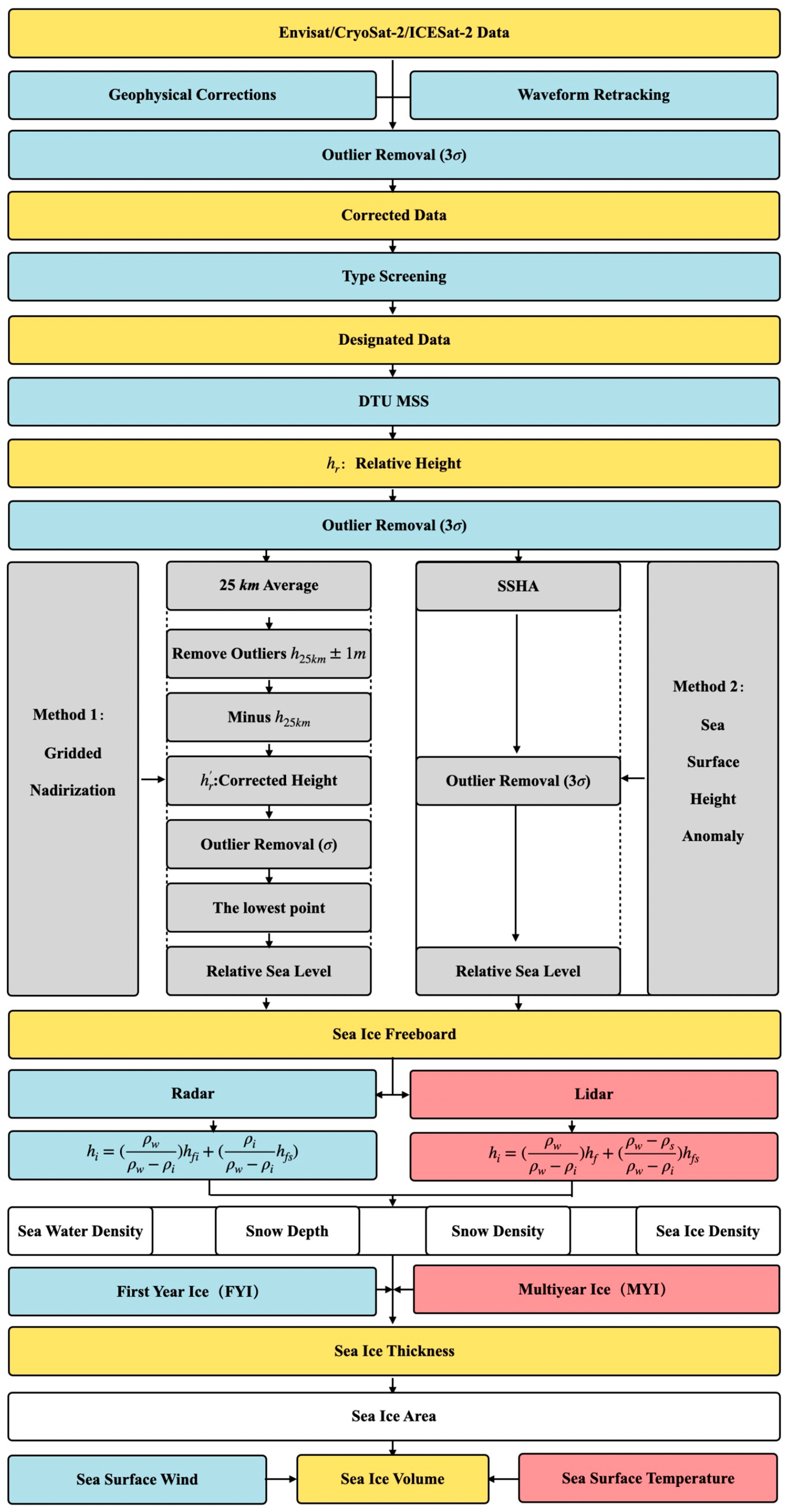
4. Methodology
4.1. Preprocessing of Altimetry Data
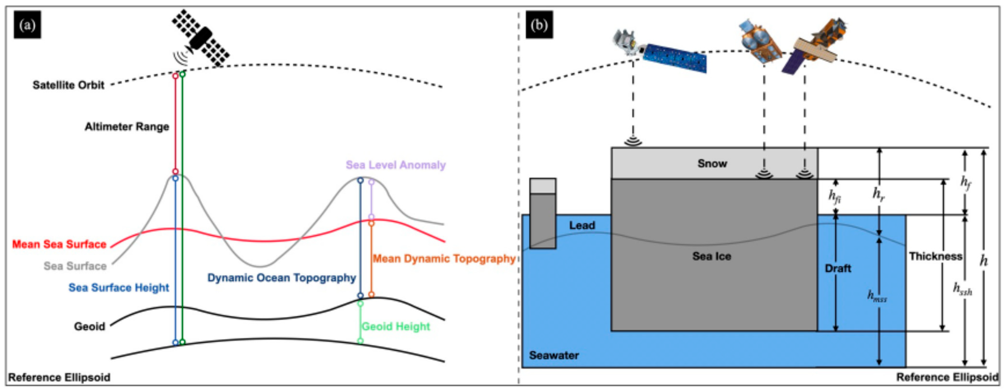
4.2. Sea Ice Freeboard Inversion Method
4.2.1. The Gridded Nadirization Method
4.2.2. Sea Surface Height Anomaly Method
4.3. Sea Ice Thickness Inversion Method
4.4. Inversion of Sea Ice Volume
5. Results and Discussion
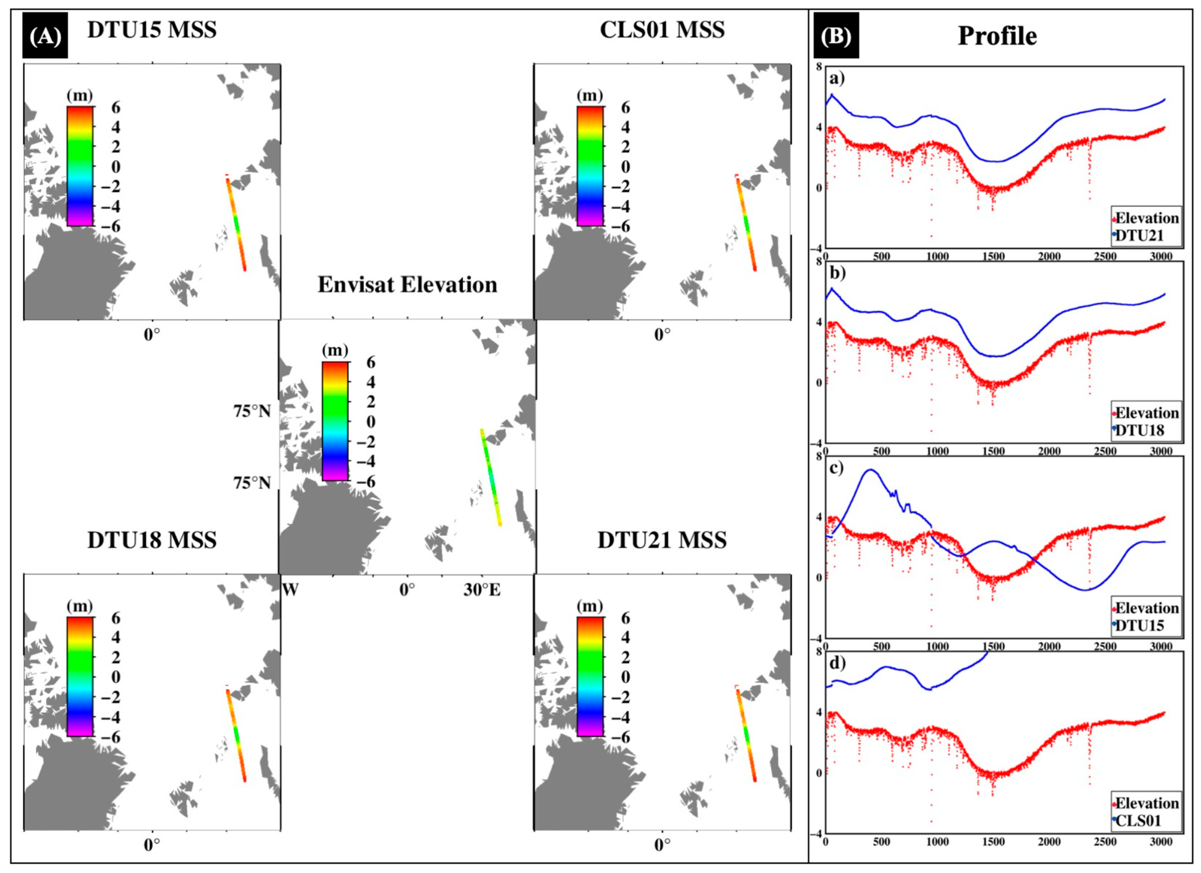
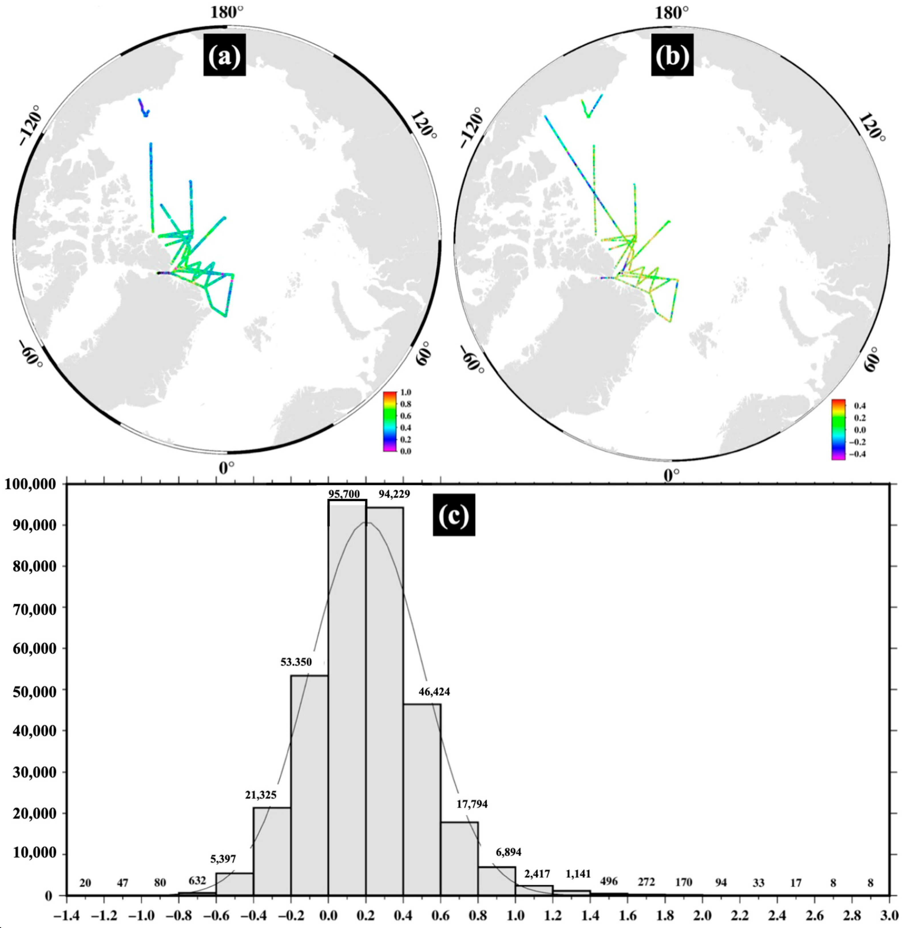
5.1. Validation and Evaluation of the MSS Height Model
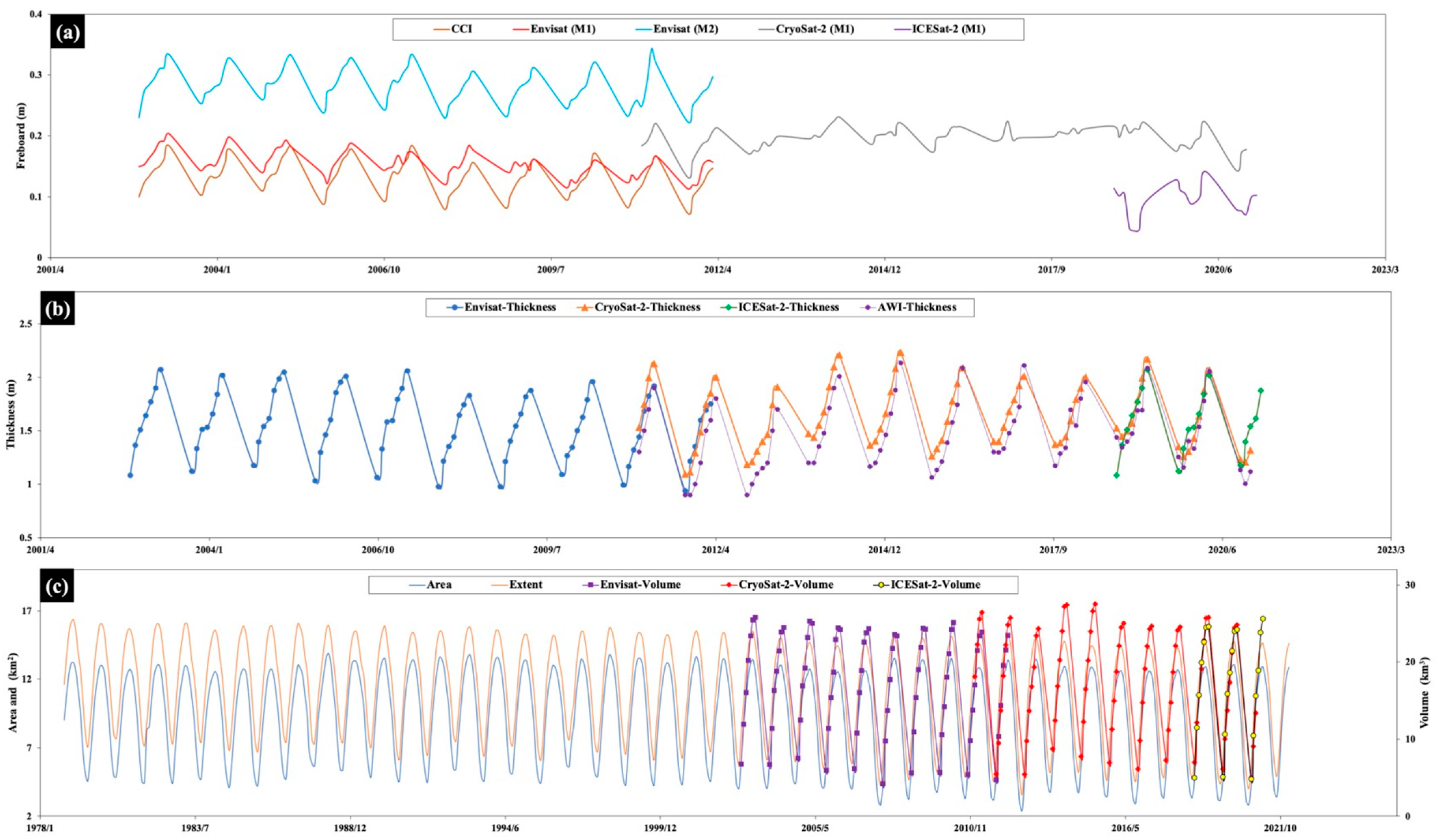
5.2. Calculation of ASI Freeboard Using Envisat/CryoSat-2/ICESat-2
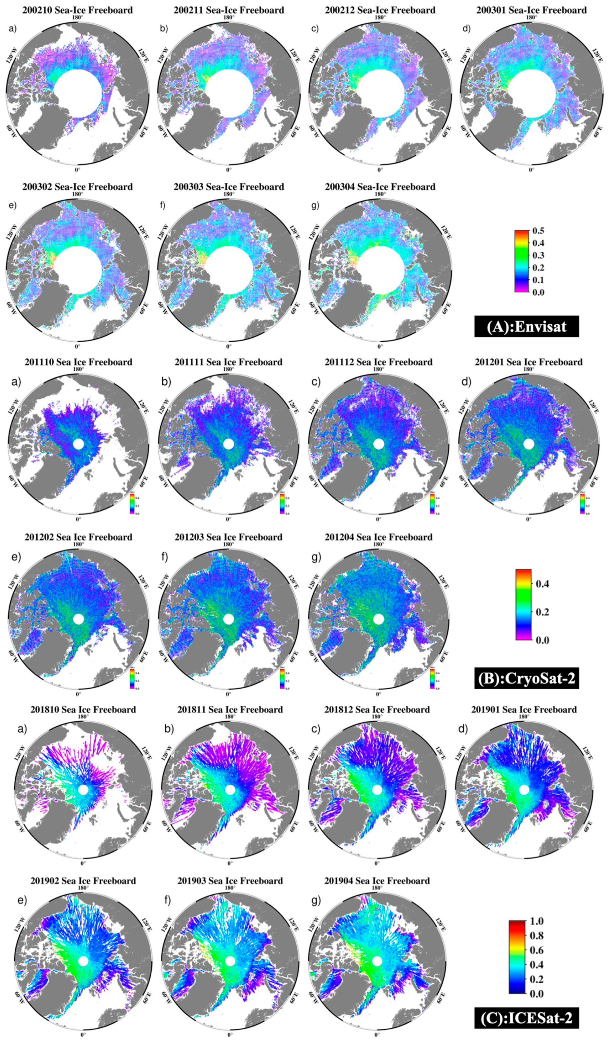
5.2.1. Using Envisat to Calculate Sea Ice Freeboard
5.2.2. Calculation of Sea Ice Freeboard Using CryoSat-2

5.2.3. Using ICESat-2 to Calculate Sea Ice Freeboard


5.3. Sea Ice Thickness
5.4. Sea Ice Volume
5.5. Analysis of Influencing Factors
5.5.1. Sea Surface Temperature
5.5.2. Surface Wind Field
6. Conclusions
Author Contributions
Funding
Institutional Review Board Statement
Informed Consent Statement
Data Availability Statement
Acknowledgments
Conflicts of Interest
References
- Dai, A.; Luo, D.; Song, M.; Liu, J. Arctic amplification is caused by sea-ice loss under increasing CO2. Nat. Commun. 2019, 10, 121. [Google Scholar] [CrossRef] [PubMed]
- Lin, Y.; Moreno, C.; Marchetti, A.; Ducklow, H.; Schofield, O.; Delage, E.; Meredith, M.; Li, Z.; Eveillard, D.; Chaffron, S.; et al. Decline in plankton diversity and carbon flux with reduced sea ice extent along the Western Antarctic Peninsula. Nat. Commun. 2021, 12, 4948. [Google Scholar] [CrossRef] [PubMed]
- Kwok, R.; Cunningham, G.F.; Wensnahan, M.; Rigor, I.; Zwally, H.J.; Yi, D. Thinning and volume loss of the Arctic Ocean sea ice cover: 2003–2008. J. Geophys. Res. Oceans 2009, 114, C07005. [Google Scholar] [CrossRef]
- Lindsay, R.; Schweiger, A. Arctic sea ice thickness loss determined using subsurface, aircraft, and satellite observations. Cryosphere 2015, 9, 269–283. [Google Scholar] [CrossRef]
- Vaughan, D.G.; Comiso, J.C.; Allison, I.; Carrasco, J.; Kaser, G.; Kwok, R.; Mote, P.; Murray, T.; Paul, F.; Ren, J.; et al. Observations: Cryosphere. In Climate Change 2013: The Physical Science Basis. Contribution of Working Group I to the Fifth Assessment Report of the Intergovernmental Panel on Climate Change; Cambridge University Press: Cambridge, UK, 2013. [Google Scholar]
- Curry, J.A.; Schramm, J.L.; Ebert, E.E. Sea ice-albedo climate feedback mechanism. J. Clim. 1995, 8, 240–247. [Google Scholar] [CrossRef]
- Sedlar, J.; Tjernström, M.; Mauritsen, T.; Shupe, M.D.; Brooks, I.M.; Persson, P.O.G.; Birch, C.E.; Leck, C.; Sirevaag, A.; Nicolaus, M. A transitioning Arctic surface energy budget: The impacts of solar zenith angle, surface albedo and cloud radiative forcing. Clim. Dyn. 2011, 37, 1643–1660. [Google Scholar] [CrossRef]
- Aagaard, K.; Carmack, E.C. The role of sea ice and other fresh water in the Arctic circulation. J. Geophys. Res. 1989, 94, 14485–14498. [Google Scholar] [CrossRef]
- Serreze, M.C.; Barrett, A.P.; Slater, A.G.; Woodgate, R.A.; Aagaard, K.; Lammers, R.B.; Steele, M.; Moritz, R.; Meredith, M.; Lee, C.M. The large-scale freshwater cycle of the Arctic. J. Geophys. Res. Oceans 2006, 111, C11010. [Google Scholar] [CrossRef]
- Brandon, M.A.; Cottier, F.R.; Nilsen, F. Sea Ice and Oceanography. In Sea Ice, 2nd ed.; Blackwell Publishing Ltd.: Hoboken, NJ, USA, 2010. [Google Scholar] [CrossRef]
- Regehr, E.V.; Hunter, C.M.; Caswell, H.; Amstrup, S.C.; Stirling, I. Survival and breeding of polar bears in the southern Beaufort Sea in relation to sea ice. J. Anim. Ecol. 2010, 79, 117–127. [Google Scholar] [CrossRef] [PubMed]
- Wadhams, P.; Wilkinson, J.P.; McPhail, S.D. A new view of the underside of Arctic sea ice. Geophys. Res. Lett. 2006, 33, L04501. [Google Scholar] [CrossRef]
- Djepa, V. Improved Retrieval of Sea Ice Thickness and Density from Laser Altimeter. Atmos. Clim. Sci. 2014, 4, 907–918. [Google Scholar] [CrossRef]
- Kwok, R. Satellite remote sensing of sea-ice thickness and kinematics: A review. J. Glaciol. 2011, 56, 1129–1140. [Google Scholar] [CrossRef]
- Francis, J.A.; Vavrus, S.J. Evidence linking Arctic amplification to extreme weather in mid-latitudes. Geophys. Res. Lett. 2012, 39, L06801. [Google Scholar] [CrossRef]
- Schweiger, O.; Settele, J.; Kudrna, O.; Klotz, S.; Kühn, I. Climate change can cause spatial mismatch of trophically interacting species. Ecology 2008, 89, 3472–3479. [Google Scholar] [CrossRef]
- Singarayer, J.S.; Bamber, J.L.; Valdes, P.J. Twenty-first-century climate impacts from a declining Arctic sea ice cover. J. Clim. 2006, 19, 1109–1125. [Google Scholar] [CrossRef]
- Laxon, S.; Peacock, H.; Smith, D. High interannual variability of sea ice thickness in the Arctic region. Nature 2003, 425, 947–950. [Google Scholar] [CrossRef] [PubMed]
- Giles, K.A.; Laxon, S.W.; Ridout, A.L. Circumpolar thinning of Arctic sea ice following the 2007 record ice extent minimum. Geophys. Res. Lett. 2008, 35, L22502. [Google Scholar] [CrossRef]
- Laxon, S.W.; Giles, K.A.; Ridout, A.L.; Wingham, D.J.; Willatt, R.; Cullen, R.; Kwok, R.; Schweiger, A.; Zhang, J.; Haas, C.; et al. CryoSat-2 estimates of Arctic sea ice thickness and volume. Geophys. Res. Lett. 2013, 40, 732–737. [Google Scholar] [CrossRef]
- Tilling, R.L.; Ridout, A.; Shepherd, A. Estimating Arctic sea ice thickness and volume using CryoSat-2 radar altimeter data. Adv. Space Res. 2018, 62, 1203–1225. [Google Scholar] [CrossRef]
- Kwok, R.; Zwally, H.J.; Yi, D. ICESat observations of Arctic sea ice: A first look. Geophys. Res. Lett. 2004, 31, L16401. [Google Scholar] [CrossRef]
- Kwok, R.; Cunningham, G.F. ICESat over Arctic sea ice: Estimation of snow depth and ice thickness. J. Geophys. Res. Oceans 2008, 113, C08010. [Google Scholar] [CrossRef]
- Kacimi, S.; Kwok, R. Arctic Snow Depth, Ice Thickness, and Volume From ICESat-2 and CryoSat-2: 2018–2021. Geophys. Res. Lett. 2022, 49, e2021GL097448. [Google Scholar] [CrossRef]
- Louet, J.; Bruzzi, S. ENVISAT mission and system. In Proceedings of the IEEE 1999 International Geoscience and Remote Sensing Symposium. IGARSS’99 (Cat. No.99CH36293), Hamburg, Germany, 28 June–2 July 1999. [Google Scholar] [CrossRef]
- Wingham, D.J.; Francis, C.R.; Baker, S.; Bouzinac, C.; Brockley, D.; Cullen, R.; de Chateau-Thierry, P.; Laxon, S.W.; Mallow, U.; Mavrocordatos, C.; et al. CryoSat: A mission to determine the fluctuations in Earth’s land and marine ice fields. Adv. Space Res. 2006, 37, 841–871. [Google Scholar] [CrossRef]
- Abdalati, W.; Zwally, H.J.; Bindschadler, R.; Csatho, B.; Farrell, S.L.; Fricker, H.A.; Harding, D.; Kwok, R.; Lefsky, M.; Markus, T.; et al. The ICESat-2 laser altimetry mission. Proc. IEEE 2010, 98, 735–751. [Google Scholar] [CrossRef]
- Baltazar Andersen, O.; Abulaitijiang, A.; Zhang, S.; Kildegaard Rose, S. A new high resolution Mean Sea Surface (DTU21MSS) for improved sea level monitoring. In EGU General Assembly Conference Abstracts; European Geosciences Union: Vienna, Austria, 2021. [Google Scholar]
- Paul, S.; Hendricks, S.; Ricker, R.; Kern, S.; Rinne, E. Empirical parametrization of envisat freeboard retrieval of arctic and antarctic sea ice based on CryoSat-2: Progress in the ESA climate change initiative. Cryosphere 2018, 12, 2437–2460. [Google Scholar] [CrossRef]
- Stefan, H.; Ricker, R.; Paul, S. AWI CryoSat-2 Sea Ice Thickness, Version 2.4; EPIC: Verona, WI, USA, 2021. [Google Scholar]
- Cavalieri, D.J.; Parkinson, C.L.; DiGirolamo, N.; Ivanoff, A. Intersensor Calibration between F13 SSMI and F17 SSMIS for Global Sea Ice Data Records. 2012. Available online: https://ntrs.nasa.gov/citations/20120009376 (accessed on 12 April 2022).
- Warren, S.G.; Rigor, I.G.; Untersteiner, N.; Radionov, V.F.; Bryazgin, N.N.; Aleksandrov, Y.I.; Colony, R. Snow depth on Arctic sea ice. J. Clim. 1999, 12, 1814–1829. [Google Scholar] [CrossRef]
- Brucker, L.; Markus, T. Arctic-scale assessment of satellite passive microwave-derived snow depth on sea ice using Operation IceBridge airborne data. J. Geophys. Res. Oceans 2013, 118, 2892–2905. [Google Scholar] [CrossRef]
- Markus, T.; Cavalieri, D.J.; Gasiewski, A.J.; Klein, M.; Maslanik, J.A.; Powell, D.C.; Boba Stankov, B.; Stroeve, J.C.; Sturm, M. Microwave signatures of snow on sea ice: Observations. IEEE Trans. Geosci. Remote Sens. 2006, 44, 3081–3090. [Google Scholar] [CrossRef]
- Comiso, J.C. Warming trends in the Arctic from clear sky satellite observations. J. Clim. 2003, 16, 3498–3510. [Google Scholar] [CrossRef]
- Petty, A.A.; Webster, M.; Boisvert, L.; Markus, T. The NASA Eulerian Snow on Sea Ice Model (NESOSIM) v1.0: Initial model development and analysis. Geosci. Model Dev. 2018, 11, 4577–4602. [Google Scholar] [CrossRef]
- Alexandrov, V.; Sandven, S.; Wahlin, J.; Johannessen, O.M. The relation between sea ice thickness and freeboard in the Arctic. Cryosphere 2010, 4, 373–380. [Google Scholar] [CrossRef]
- Farrell, S.L.; Kurtz, N.; Connor, L.N.; Elder, B.C.; Leuschen, C.; Markus, T.; McAdoo, D.C.; Panzer, B.; Richter-Menge, J.; Sonntag, J.G. A first assessment of IceBridge Snow and Ice thickness data over arctic sea ice. IEEE Trans. Geosci. Remote Sens. 2012, 50, 2098–2111. [Google Scholar] [CrossRef]
- Timco, G.W.; Frederking, R.M.W. A review of sea ice density. Cold Reg. Sci. Technol. 1996, 24, 1–6. [Google Scholar] [CrossRef]
- Arfeuille, G.; Mysak, L.A.; Tremblay, L.B. Simulation of the interannual variability of the wind-driven Arctic sea-ice cover during 1958–1998. Clim. Dyn. 2000, 16, 107–121. [Google Scholar] [CrossRef]
- Comiso, J.C.; Cavalieri, D.J.; Markus, T. Sea ice concentration, ice temperature, and snow depth using AMSR-E data. IEEE Trans. Geosci. Remote Sens. 2003, 41 Pt 1, 243–252. [Google Scholar] [CrossRef]
- Visbeck, M.H.; Hurrell, J.W.; Polvani, L.; Cullen, H.M. The North Atlantic oscillation: Past, present, and future. Proc. Natl. Acad. Sci. USA 2001, 98, 12876–12877. [Google Scholar] [CrossRef]
- Kalnay, E.; Kanamitsu, M.; Kistler, R.; Collins, W.; Deaven, D.; Gandin, L.; Iredell, M.; Saha, S.; White, G.; Woollen, J.; et al. The NCEP/NCAR 40-year reanalysis project. Bull. Am. Meteorol. Soc. 1996, 77, 437–472. [Google Scholar] [CrossRef]
- Faugere, Y.; Dorandeu, J.; Lefevre, F.; Picot, N.; Femenias, P. Envisat Ocean Altimetry Performance Assessment and Cross-calibration. Sensors 2006, 6, 100–130. [Google Scholar] [CrossRef]
- Wingham, D.J.; Rapley, C.G.; Griffiths, H. New Techniques in Satellite Altimeter Tracking Systems. In Proceedings of the Digest—International Geoscience and Remote Sensing Symposium (IGARSS), Zürich, Switzerland, 8–11 September 1986. [Google Scholar]
- Kwok, R.; Petty, A.; Bagnardi, M.; Wimert, J.T.; Cunningham, G.F.; Hancock, D.W.; Ivanoff, A.; Kurtz, N. Algorithm Theoretical Basis Document (ATBD) for Sea Ice Products; National Aeronautics and Space Administration: Washington, DC, USA, 2022.
- Pukelsheim, F. The three sigma rule. Am. Stat. 1994, 48, 88–91. [Google Scholar] [CrossRef]
- Ollivier, A.; Faugere, Y.; Picot, N.; Ablain, M.; Femenias, P.; Benveniste, J. Envisat Ocean Altimeter Becoming Relevant for Mean Sea Level Trend Studies. Mar. Geod. 2012, 35 (Suppl. 1), 118–136. [Google Scholar] [CrossRef]
- Kwok, R.; Cunningham, G.F.; Zwally, H.J.; Yi, D. Ice, Cloud, and land Elevation Satellite (ICESat) over Arctic sea ice: Retrieval of freeboard. J. Geophys. Res. Oceans 2007, 112, C12013. [Google Scholar] [CrossRef]
- Farrell, S.L.; Laxon, S.W.; McAdoo, D.C.; Yi, D.; Zwally, H.J. Five years of arctic sea ice freeboard measurements from the ice, cloud and land elevation satellite. J. Geophys. Res. Oceans 2009, 114, C04008. [Google Scholar] [CrossRef]
- Beaven, S.G.; Lockhart, G.L.; Gogineni, S.P.; Hosseinmostafa, A.R.; Jezek, K.; Gow, A.J.; Perovich, D.K.; Fung, A.K.; Tjuatja, S. Laboratory measurements of radar backscatter from bare and snow-covered saline ice sheets. Int. J. Remote Sens. 1995, 16, 851–876. [Google Scholar] [CrossRef]
- Agarwal, P.K.; Avraham, R.; Ben Kaplan, H.; ShCPir, M. Computing the discrete fréchet diStance in subquadratic time. SIAM J. Comput. 2014, 43, 429–449. [Google Scholar] [CrossRef]
- Landy, J.C.; Dawson, G.J.; Tsamados, M.; Bushuk, M.; Stroeve, J.C.; Howell, S.E.L.; Krumpen, T.; Babb, D.G.; Komarov, A.S.; Heorton, H.D.B.S.; et al. A year-round satellite sea-ice thickness record from CryoSat-2. Nature 2022, 609, 517–522. [Google Scholar] [CrossRef]
- Li, M.; Luo, D.; Simmonds, I.; Dai, A.; Zhong, L.; Yao, Y. Anchoring of atmospheric teleconnection patterns by Arctic Sea ice loss and its link to winter cold anomalies in East Asia. Int. J. Climatol. 2021, 41, 547–558. [Google Scholar] [CrossRef]
- Hilmer, M.; Lemke, P. On the decrease of Arctic Sea ice volume. Geophys. Res. Lett. 2000, 27, 3751–3754. [Google Scholar] [CrossRef]
- Schweiger, A.J.; Wood, K.R.; Zhang, J. Arctic Sea Ice volume variability over 1901–2010: A model-based reconstruction. J. Clim. 2019, 32, 4731–4752. [Google Scholar] [CrossRef]


| MSS Model | Level of Dissimilarity |
|---|---|
| CLS01 | 7.8639 |
| DTU15 | 7.9878 |
| DTU18 | 12.0550 |
| DTU21 | 2.9542 × 10³ |
| N = 3 | N = 2 | N = 1 | N = 0.5 | ||||||
|---|---|---|---|---|---|---|---|---|---|
| Grid | Total Number of Original Points | Total Number after Filtered Points | Rejection Rate (%) | Total Number of Filtered Points | Rejection Rate (%) | Total Number after Filtered Points | Rejection Rate (%) | Total Number after Filtered Points | Rejection Rate (%) |
| Sample1 | 16,476 | 15,888 | 3.56 | 15,249 | 7.45 | 11,802 | 28.37 | 6717 | 59.23 |
| Sample2 | 16,965 | 16,431 | 3.14 | 15,714 | 7.34 | 12,363 | 27.13 | 6927 | 59.17 |
| Sample3 | 15,302 | 14,738 | 3.68 | 14,328 | 6.37 | 12,187 | 20.36 | 6950 | 54.58 |
| Sample4 | 16,353 | 15,678 | 4.12 | 15,135 | 7.45 | 12,012 | 26.55 | 6345 | 61.20 |
| Sample5 | 16,806 | 16,008 | 4.74 | 15,480 | 7.89 | 11,997 | 25.43 | 6636 | 60.51 |
| Month | CCI | |||||
|---|---|---|---|---|---|---|
| Gridded Nadirization | SSHA | |||||
| October | Bias/m | RMSE/m | STD/m | Bias/m | RMSE/m | STD/m |
| November | 0.12 | 0.15 | 0.09 | 0.25 | 0.30 | 0.29 |
| December | 0.12 | 0.14 | 0.08 | 0.25 | 0.30 | 0.28 |
| January | 0.11 | 0.14 | 0.08 | 0.24 | 0.28 | 0.28 |
| February | 0.11 | 0.13 | 0.08 | 0.24 | 0.28 | 0.27 |
| March | 0.09 | 0.13 | 0.09 | 0.18 | 0.20 | 0.27 |
| April | 0.10 | 0.14 | 0.10 | 0.19 | 0.21 | 0.28 |
| Overall | 0.11 | 0.14 | 0.09 | 0.22 | 0.22 | 0.28 |
Disclaimer/Publisher’s Note: The statements, opinions and data contained in all publications are solely those of the individual author(s) and contributor(s) and not of MDPI and/or the editor(s). MDPI and/or the editor(s) disclaim responsibility for any injury to people or property resulting from any ideas, methods, instructions or products referred to in the content. |
© 2023 by the authors. Licensee MDPI, Basel, Switzerland. This article is an open access article distributed under the terms and conditions of the Creative Commons Attribution (CC BY) license (https://creativecommons.org/licenses/by/4.0/).
Share and Cite
Zhang, Y.; Chao, N.; Li, F.; Yue, L.; Wang, S.; Chen, G.; Wang, Z.; Yu, N.; Sun, R.; Ouyang, G. Reconstructing Long-Term Arctic Sea Ice Freeboard, Thickness, and Volume Changes from Envisat, CryoSat-2, and ICESat-2. J. Mar. Sci. Eng. 2023, 11, 979. https://doi.org/10.3390/jmse11050979
Zhang Y, Chao N, Li F, Yue L, Wang S, Chen G, Wang Z, Yu N, Sun R, Ouyang G. Reconstructing Long-Term Arctic Sea Ice Freeboard, Thickness, and Volume Changes from Envisat, CryoSat-2, and ICESat-2. Journal of Marine Science and Engineering. 2023; 11(5):979. https://doi.org/10.3390/jmse11050979
Chicago/Turabian StyleZhang, Yanze, Nengfang Chao, Fupeng Li, Lianzhe Yue, Shuai Wang, Gang Chen, Zhengtao Wang, Nan Yu, Runzhi Sun, and Guichong Ouyang. 2023. "Reconstructing Long-Term Arctic Sea Ice Freeboard, Thickness, and Volume Changes from Envisat, CryoSat-2, and ICESat-2" Journal of Marine Science and Engineering 11, no. 5: 979. https://doi.org/10.3390/jmse11050979
APA StyleZhang, Y., Chao, N., Li, F., Yue, L., Wang, S., Chen, G., Wang, Z., Yu, N., Sun, R., & Ouyang, G. (2023). Reconstructing Long-Term Arctic Sea Ice Freeboard, Thickness, and Volume Changes from Envisat, CryoSat-2, and ICESat-2. Journal of Marine Science and Engineering, 11(5), 979. https://doi.org/10.3390/jmse11050979