Echoes of the 2013–2015 Marine Heat Wave in the Eastern Bering Sea and Consequent Biological Responses

Abstract

We reviewed various physical and biological manifestations of an unprecedented large-scale water temperature anomaly that emerged in the Northeast Pacific in late 2013. The anomaly dubbed “The Blob” persisted through 2014–2016, with some signs of its persistence through 2017–2018 and a possible reemergence in 2019. The tentative timeline of The Blob’s successive appearances around the Northeast Pacific is suggestive of its advection by currents around the Gulf of Alaska, along the Aleutians, into the Bering Sea, and eventually to the Bering Strait. During the initial phase of The Blob’s development in 2013–2014, advection along the Polar Front might have played a certain role. The extreme persistence and magnitude of The Blob resulted in numerous and sometimes dramatic ecosystem responses in the eastern Bering Sea. The multi-year duration of The Blob might have preconditioned the Bering Sea for the record low seasonal sea ice extent during the winter of 2017–2018 and the disappearance of the cold pool in 2016 and 2018 that profoundly affected zooplankton, invertebrates, fishes, seabirds, and marine mammals. A comparison of the time series of population responses across trophic levels suggests that The Blob lowered primary production during spring, increased production of small copepods and jellyfish, and reduced the efficiency of energy transfer to higher trophic levels. While the Bering Sea’s water temperature, seasonal sea ice, and cold pool seem to return to the long-term mean state in 2022, it remains to be seen if the Bering Sea ecosystem will completely recover. The two most likely alternative scenarios envision either irreversible changes or hysteresis recovery.

1. Introduction

An unprecedented large-scale warm-water anomaly emerged in the NE Pacific in late 2013 as documented by Freeland (2014) [1], Freeland (2015) [2], and Freeland and Ross (2019) [3]. It was first reported by Freeland (2014) [1] based on (a) Argo data along Line P and (b) sea surface temperature (SST) data, both from January 2014, when SST anomaly in the Gulf of Alaska exceeded four standard deviations (Figure 1). As Freeland (2014) noted ([1], p. 58): “Four standard deviations away from the mean state is HUGE. … Again we see huge deviations from normal conditions with temperature in January 2014 4.4 standard deviations above the mean, salinity 3 standard deviations below the mean and as a consequence of both low salinity and high temperature, we see extremely low surface density by 4.4 standard deviations.”

During 2014, this anomaly dubbed “The Blob” by Bond et al. (2015) [4] shifted east and north, and by June 2014 reached the Bering Sea (Figure 2) as documented by Freeland (2015) ([2], Figure 6-1).

The Blob lasted through 2016 in the upper 0–100 m layer yet lingered through 2017–2018 in the subsurface 100–200 m layer, as documented by Freeland and Ross (2019) [3], who also noted a possible return in late 2018 of a warm anomaly (Figure 3), which actually occurred in 2019 as reported by Scannell et al. (2020) [5]. During the first years, The Blob’s manifestation in the surface layer diminished, while its manifestation in the subsurface markedly increased as noted by Freeland and Ross (2019) [3], Zhi et al. (2019) [6], and Holser et al. (2022) [7], among others (Figure 3).

The Blob’s impact on the marine ecology of the Northeast Pacific was dramatic in terms of magnitude, duration, and spatial extent. Ecosystem implications of The Blob are well documented in the California Current by Cavole et al. (2016) [8] and around the Gulf of Alaska (GOA) by Suryan et al. (2021) [9]. Less is known about the physical and biological manifestations of The Blob in the Bering Sea, particularly in the Eastern Bering Sea (EBS) and Northern Bering Sea (NBS), largely because of the uncertain timeline of The Blob’s propagation from the open Northeast Pacific to the Bering Sea. The present review is an attempt to address this issue.

Given the regional circulation pattern that connects the GOA with EBS via the Alaskan Stream, Aleutian Current, and Aleutian North Slope Current (Figure 4), one would expect to see surface waters affected by The Blob in the open Northeast Pacific to be advected by the above currents into the southeastern Bering Sea and farther downstream, along the EBS Shelf, all the way to the Bering Strait. In the first part of this paper, we review the available evidence of The Blob’s propagation to the Bering Sea and eventually to the Bering Strait. We also review publicly available data on SST, sea ice cover, and cold pool on the EBS Shelf, as well as other physical factors that directly or indirectly affect marine biota. In the second part of this paper, we review the ecological consequences of The Blob’s propagation to and across the Bering Sea, with a strong focus on the EBS Shelf (EBSS) and NBS Shelf (NBSS).

2. Data and Methods

We reviewed English-language literature on The Blob and its physical and biological ramifications in the Northeast Pacific, from the Gulf of Alaska to the Bering Sea and Bering Strait. While our main focus was on the peer-review papers published in academic journals, we also searched for data and data analyses in the gray literature, particularly in regular ecosystem assessments published by the NOAA. Since this review is squarely focused on The Blob, which emerged in 2013, our time scope was limited to the last decade, from 2013 until now. Rare exceptions were made for papers describing similar anomalies in the past; a comparison of such anomalies with The Blob can be quite useful.

Numerous biological consequences of The Blob were reported in the literature, including The Blob’s effects on zooplankton and ecologically significant and commercially important species of fish and invertebrates, their life stages, and species-specific and ontogeny-associated spatial shifts in distribution and abundance reviewed by Mueter et al. (2021) [12] and Suryan et al. (2021) [9]. Biological events linked (hypothetically or conclusively) to The Blob’s passage include phytoplankton blooms such as coccolithophore blooms reviewed by Ladd et al. (2018) [13] and Matson et al. (2019) [14], and toxic algal blooms (harmful algal blooms, HABs) reported by Peterson et al. (2016) [15]. In turn, toxic algal blooms cause mass die-offs of seabirds and marine mammals (e.g., whales).

3. Formation, Evolution, and Propagation of the Blob to the Bering Sea

Results of our review are arranged along-stream, presenting evidence of The Blob and documenting a timeline of The Blob’s propagation from the open Northeast Pacific into the Bering Sea, then along the EBS Shelf to the Bering Strait. Naturally, the downstream narrative is ordered chronologically.

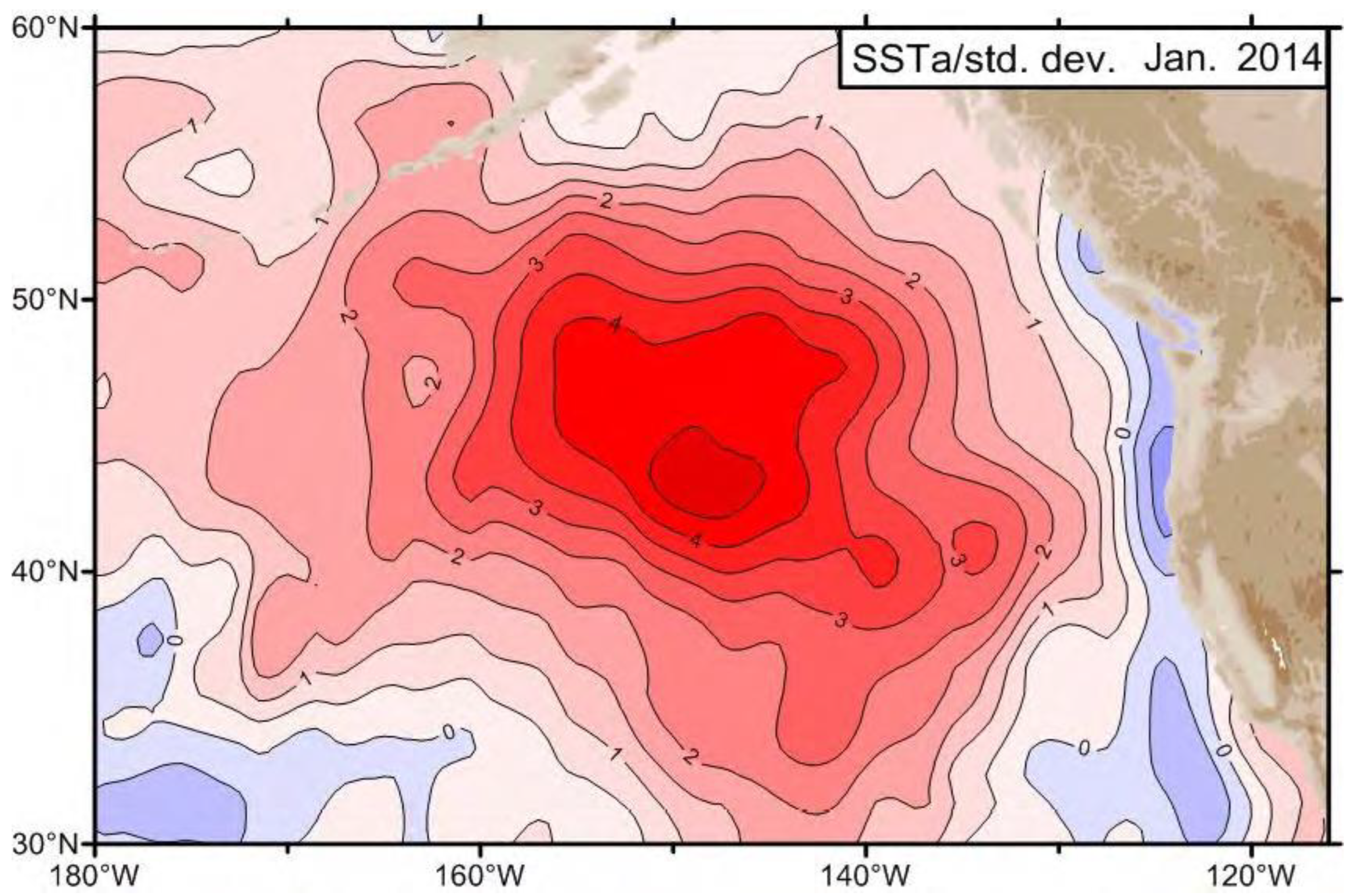
3.1. The Blob’s Emergence and Early Detection

The Blob’s sudden emergence at Ocean Station Papa (OSP) in late 2013 was analyzed in detail by Freeland and Ross (2019) [3] who noted ([3], p. 5): “Figure 5 shows the very sudden onset of The Blob at the end of 2013 and that it was fully present in January 2014. This agrees with the sudden onset seen in the SST maps (Figure 1).” Freeland and Ross (2019) [3] also noted that “a large salinity anomaly occurs at the same time and this anomaly is not density-compensating, rather there is a large fresh anomaly with salinity departing from the mean by 3.0 standard deviations. The result is that a very large density anomaly occurs with the surface waters becoming less dense by 4.3 standard deviations. … The result was the creation of a substantial barrier to wind-induced mixing and as the mixed-layer deepening season progressed through early 2014, with low storm activity, we saw anomalously shallow mixed layers.” ([3], p. 6). In absolute terms, the near-surface salinity in January 2014 was 32.45 psu, a drop of 0.2 in a year from the mean surface salinity of 34.65 psu in 2007–2013. The stratification barrier notwithstanding, The Blob gradually extended to the subsurface over 2014–2016 as documented by Freeland and Ross (2019) [3]. Temperature and salinity data collected in 2014–2017 by instrumented northern elephant seals in the Northeast Pacific were analyzed by Holser et al. (2022) [7] to provide evidence of The Blob extending eventually to 1000 m depth. The vertical extent of The Blob is essential with regard to its propagation to the Bering Sea via the Aleutian Straits where the shallow depths of some passes will constrain water transport as discussed below; for more information, see the latest geomorphological study of the Aleutian passes by Zimmerman and Prescott (2021) [16].

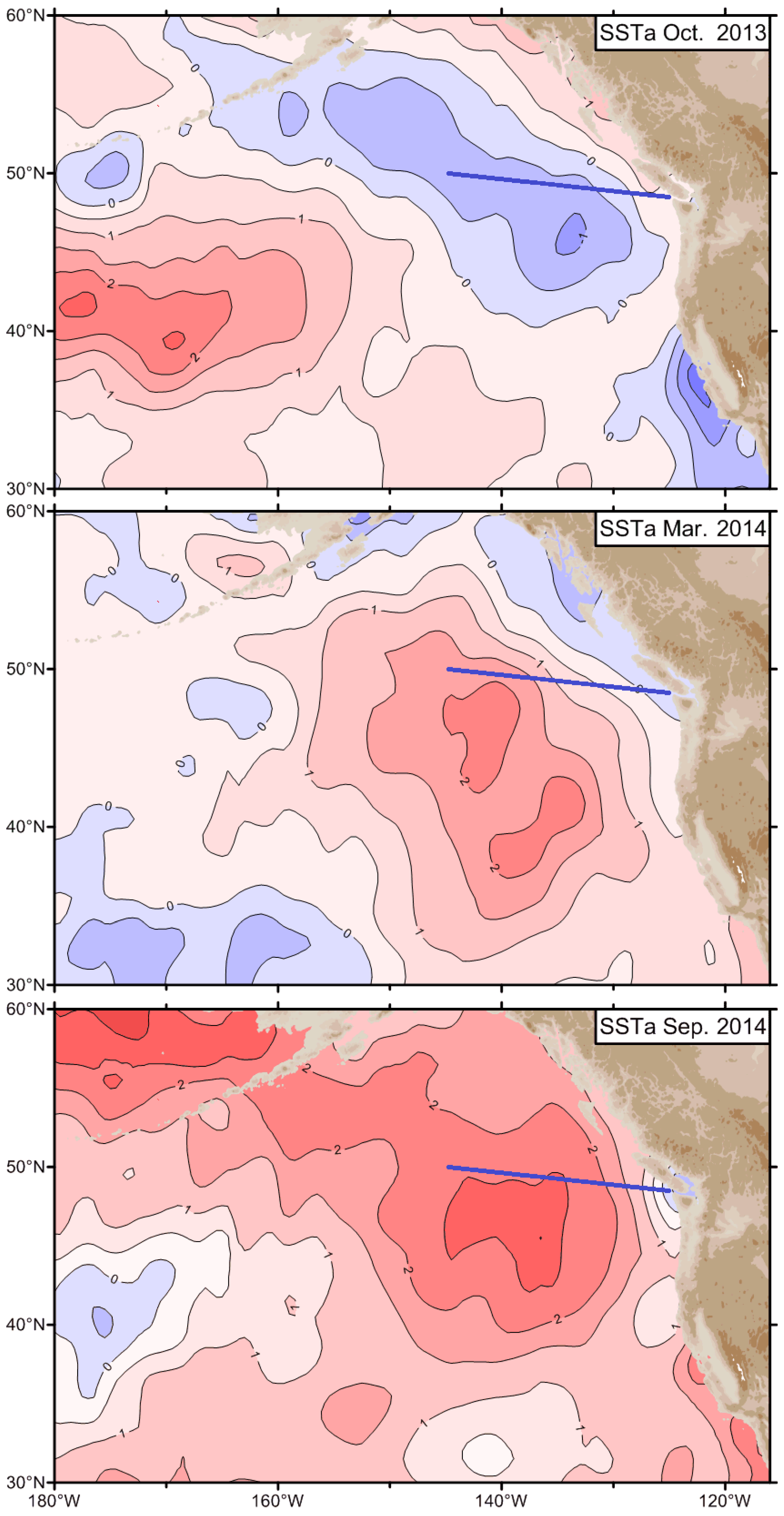
3.2. The Blob’s Preconditioning in the Central North Pacific

Zhi et al. (2019) [6] have shown that The Blob’s appearance as a temperature anomaly was preceded and actually preconditioned by a large negative salinity anomaly in the central North Pacific that originated in 2010–2011 in the western Pacific. This salinity anomaly played a key role during 2012–2013 in the observed formation of a shallow mixed layer in the Northeast Pacific and the emergence of a large SST anomaly (The Blob) by trapping heat in the shallow mixed layer. The shallow mixed-layer anomaly was more dependent on the local subsurface salinity anomaly in the 100–150 m layer, which was much stronger than the surface salinity anomaly. Zhi et al. (2019) [6] have shown that the salinity anomaly in the 100–150 m layer originated west of the dateline, where it was freshened, subducted, and advected eastward.

3.3. The Blob’s Advection along the Polar Front

The propagation path of The Blob across the North Pacific tentatively traced by Zhi et al. (2019) [6] lies near the long-term mean path of the Polar Front (PF) mapped by Belkin et al. (2002) [17] from >200 hydrographic sections (Figure 5); therefore, The Blob’s propagation to the northeast might have been facilitated by a geostrophic current associated with the PF.

Advection of SST anomalies along the PF was studied by Belkin and Shotwell (2012) [18] and Shotwell et al. (2014) [19]. The Polar Front Current associated with the PF acts as a conduit of oceanic anomalies originating in the Northwest Pacific. These anomalies propagate along the PF into the GOA where the PF retroflects and extends westward along the GOA shelf towards the Aleutians and into the Bering Sea. The Polar Front Current carries relatively warm waters into the GOA and to the Aleutians; therefore, intensification (relaxation) of the Polar Front Current results in warming (cooling) of the high-latitude Northeast Pacific. The succession of annual advective events in 1956–1966 was followed by a 20-year relaxation epoch, except for the 1971–1972 cold anomaly that traveled around the GOA and along the Aleutians. In 1986–1987, a major cold anomaly propagated into the GOA. The eastward advection episodes in 1990–1991 (warm and cold) and 1994 (warm) were followed by a major propagation event in 1996–1997 that culminated in an exceptionally strong warm event in the GOA in 1997 when SST anomaly south of Kodiak exceeded +2.5 °C.

3.4. The Blob’s Expansion into the Gulf of Alaska and Its Advection by Coastal Currents

The series of selected monthly SSTA maps presented by Freeland (2015) [2] and Freeland and Ross (2019) [3] reveal a northward expansion of The Blob into the GOA and an eastward shift of The Blob towards the west coast of North America (Figure 2), where SSTA exceeded +6 °C off southern California (Gentemann et al., 2017) [20]. As a result of The Blob’s shift east and north, its eastern and northern peripheries have become subjected to the advection by the poleward eastern limb of the Alaska Gyre and adjoining poleward coastal currents such as the Vancouver Island Coastal Current, the Haida Current, and the Alaska Coastal Current. Therefore, The Blob’s manifestation in coastal SST records can be expected all the way around the GOA, along the Alaska Peninsula, and along the Aleutian Islands. Indeed, in Prince William Sound, a robust cold-to-warm-epoch transition occurred in late 2014, consistent with the occupation of the Sound by The Blob (Figure 6) after the cold epoch of 2006–2013 abruptly ended in June 2013 with the arrival of The Blob’s leading edge. Downstream from the Prince William Sound, along the Seward Line, a warm temperature anomaly of unprecedented magnitude and duration was recorded in 2013–2018, consistent with The Blob’s advection by the Alaska Coastal Current (Figure 7).

Our view of The Blob’s advection by coastal currents around the GOA is shared by Walsh et al. (2018) ([22], pp. S41–S42): “The warming was primarily confined to the inner GOA shelf in September 2014, suggesting that heat was advected along-shore within the Alaska Coastal Current. By spring 2015 the shelf was uniformly warm and water remained 1°–2 °C warmer than normal through September 2016.”

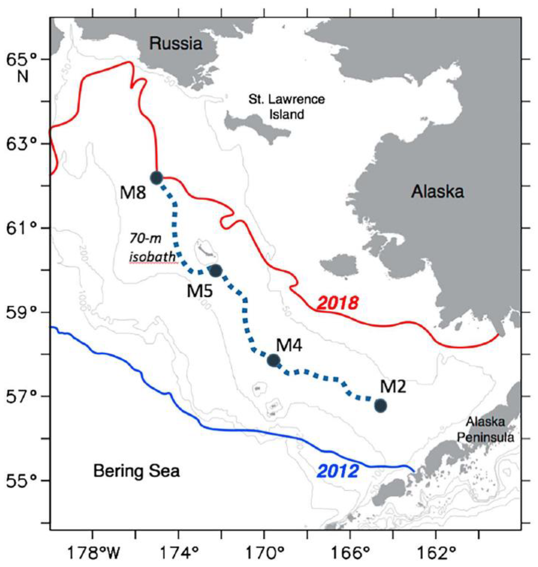
3.5. The Blob’s Propagation into the Bering Sea and towards the Bering Strait

The Blob appeared in the southern Bering Sea in June 2014, when SSTA reached three standard deviations at 180° W, then moved east (likely advected by the Aleutian North Slope Current) to occupy Bristol Bay in August 2014 (Figure 2). Stabeno et al. (2016) [23] concluded that there are two principal pathways for the Pacific waters into the Bering Sea: one (major) via Unimak Pass at 164° W and another (minor) via Amukta Pass at 172° W. Stabeno et al. (2016) [23] estimated that “A typical transit type from Unimak Pass to Bering Strait is >13 months, and from Amukta Pass to Bering Strait via the Bering Slope Current is >8 months.” ([23], p. 13). These estimates are essential to the timeline of The Blob’s propagation along the EBSS as The Blob was carried by ocean currents.

The precise timeline of The Blob’s propagation into the Bering Sea and onto the EBSS is especially important since the cold epoch of 2006–2013 ended almost simultaneously with The Blob’s penetration into the Bering Sea and EBSS. The available time series of physical parameters (SST, sea ice extent, bottom temperature, cold pool extent, etc.) can sometimes be interpreted variously. Depending on an interpretation, the cold-to-warm-epoch transition in 2013–2014 was either (a) triggered by The Blob, or (b) initiated independently from The Blob and before The Blob’s arrival at the EBS, and then reinforced by The Blob.

The Bering Sea had a long memory of The Blob’s passage. The Blob’s residence time in the EBS exceeded at least twice the advection time over which the Bering Slope Current and EBS shelf currents would carry The Blob to the Bering Strait. Indeed, as estimated by Stabeno et al. (2016) [23], the transit time from Unimak Pass and Amukta Pass to the Bering Strait varies between >13 and >8 months, respectively (roughly a year). Yet The Blob persisted in the EBS for at least two years (from mid-2014 to 2016) as evidenced by Figure 8.

3.6. Unprecedented Loss of Seasonal Sea Ice

The enhanced ocean-atmosphere heat flux and atmospheric circulation over the Bering Sea during these years resulted in an unprecedented loss of seasonal sea ice (Figure 9 and Figure 10).

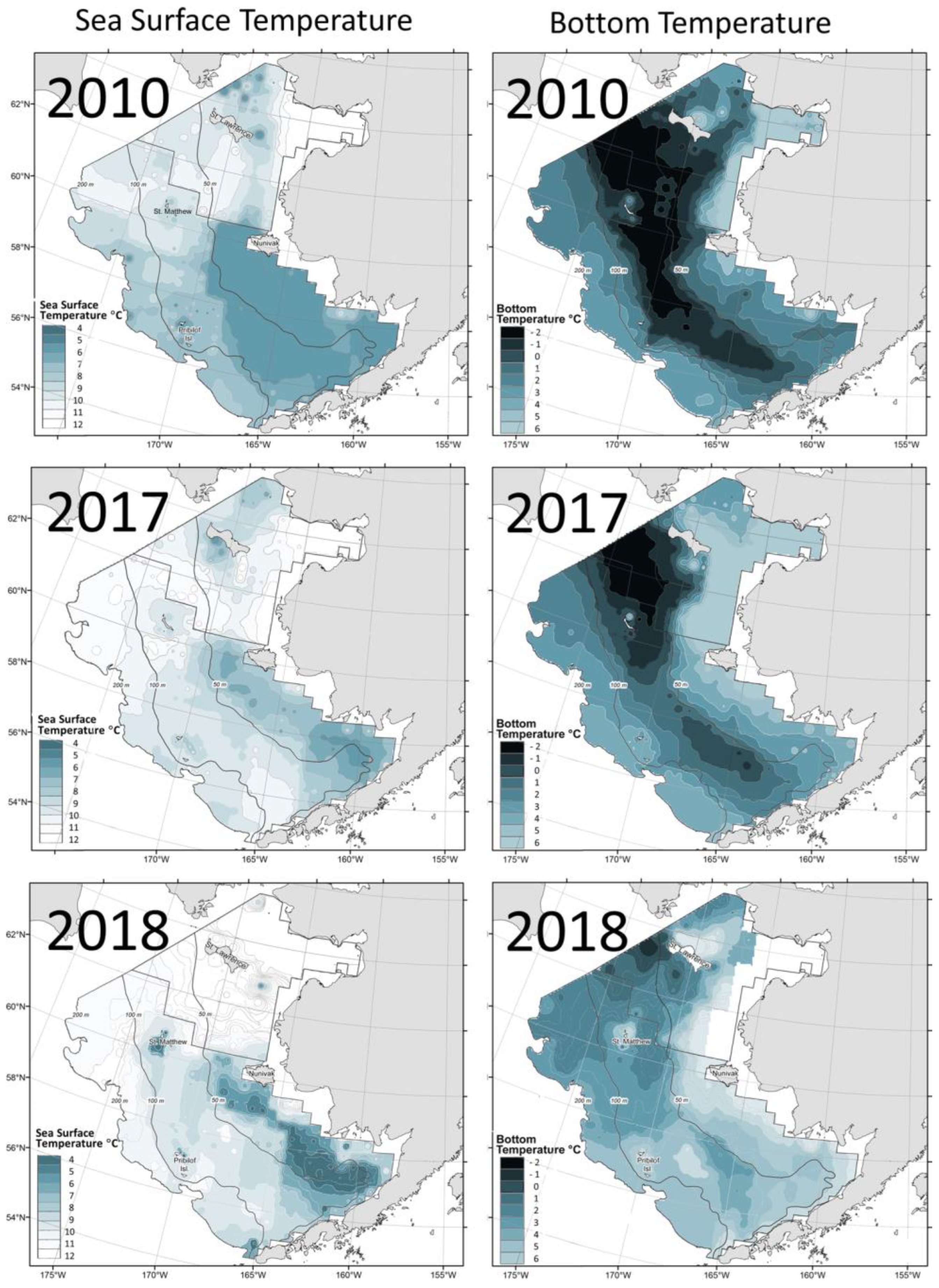
3.7. Disappearance of the Cold Pool on the East Bering Sea Shelf

The time series of annual mean anomalies of SST (SSTA) and bottom temperature (BTA) in the EBSS presented by Baker (2021) [26] reveal a rapid cold-to-warm-epoch transition in 2014–2016, with both SSTA and BTA peaking in 2016 at about 3 °C and 2 °C, respectively (Figure 11).

Baker (2021) [26] documented a stark contrast between surveys in 2010 and 2017–2018: not only had the water temperature risen sharply, but the cold pool which occupied a large area in 2010 had all but disappeared in 2018 as well (Figure 12).

Thorson (2019) [27] constructed a series of annual maps (1982–2017) of bottom temperature in 200 nodes of a quasi-regular grid covering the EBS (Figure 13). These maps show large cold pools during the cold epoch of 2006–2013, then the abrupt shrinking of the cold pool in 2014–2015, and a nearly complete disappearance of the cold pool in 2016. Duffy-Anderson et al. (2019) [25] published yet another map of the cold pool in 2018 (Figure 14) that shows its complete disappearance on the EBSS. The maps of bottom temperature on the EBSS published by Duffy-Anderson et al. (2019) [25], Thorson (2019) [27], and Baker (2021) [26] make evident the disappearance of the cold pool in 2016, its partial recovery in 2017, and disappearance again in 2018.

Johnson et al. (2022) [28] conducted the first long-term monitoring study using acoustics and ancillary oceanographic data (bottom temperature and regional seasonal sea ice (SSI) data) to study the relationship between biological scattering communities and variations in the EBS cold pool across two climate regimes, a cold one (2006–2013) and a warm one (2014–2018). They concluded ([28], p. 210): “In the fall of 2013, the EBS encountered a regime shift that was characterized by less SSI, early receding SSI, increased bottom temperatures, and a zooplankton community structure shift.”

3.8. Long-Term Variability of the Bering Shelf

Changes in the entire Bering Shelf over seasonal to century-long time scales have been recently assessed by Danielson et al. (2020) [29], who assembled and analyzed a new temperature–salinity climatology of the Bering and Chukchi Sea shelves from a half-century (1966–2018) hydrographic database. The Bering Shelf is dominated by decadal-scale variability that precludes the detection of a water column trend. However, SST shows a warming trend of 0.22 plus/minus 0.10 °C/decade. Heat fluxes in 1979–2018 exhibit no record-length trend over the Bering Sea shelf.

The Bering Sea experienced record-high SST in 2014 (Stabeno et al., 2017) [30], which persisted into 2018 (Thoman et al., 2020) [24] and 2019 (Stabeno and Bell, 2019) [31]. The upper ocean (0–300 m) integrated heat content anomalies in the EBS were correlated with SST anomalies (Walsh et al., 2018) [22].

3.9. Physical Fronts

Physical fronts have long been recognized as critically important structural and biophysical components of the Bering Sea ecosystem (Belkin and Cornillon, 2005 [32]; Hunt et al., 2008 [33]; Belkin, 2016 [11]), especially over the broad EBSS, where a few fronts of different physical nature co-exist, waxing and waning as the season progresses (Figure 15). These fronts, in particular their characteristic temperature ranges, must have been affected by a major SST anomaly associated with The Blob’s passage. Additionally, the recent dramatic reduction in the seasonal ice cover must have affected those fronts whose locations and dynamics are related to the seasonal ice edge (marginal ice zone).

4. Ecosystem Responses to The Blob in the Eastern Bering Sea

Detection of population-level responses perturbed by The Blob following its entry into the Bering Sea in July 2014 largely depends on the availability of decadal or longer time series, on the life stage most vulnerable to perturbation, and on the duration of any lag between the perturbed and monitored life stages. Time-series records that pre-date the onset of The Blob in the Bering Sea by at least a few years provide context for evaluating any ensuing changes. Detection of biotic responses may be evident within the same season, or delayed if monitored life stages are months or years older than the age of an organism’s initial response. Knowledge of such lags informs expectations of when detectable responses should be evident had a perturbation occurred, and the time scale for when they should subside.

In this section we evaluate published records of population-related time series for monitored biota in the eastern Bering Sea that pre-date 2014 by several years, and for which expected lags between the initial effects of The Blob and its expected subsequent appearance in the monitoring records are well established. Most of these records are summarized in the 2022 Ecosystem Status Report edited by Siddon (2022) [34]. We begin with a consideration of primary productivity and progress through successively higher trophic levels.

4.1. Primary Productivity

Trends in primary productivity from 2003 to 2022 have been evaluated from ocean color data provided by the satellite-based Moderate Resolution Imaging Spectroradiometer (MODIS) and averaged over spring (April–June) for eight subregions in the Bering Sea (Figure 16; Nielsen et al., 2022 [35]). Spring chlorophyll-a concentrations were consistently below the long-term median after 2014 in the off-shelf (>200 m depth) subregion (Figure 16), which includes most of the highly productive Bering Sea Green Belt (Springer et al., 1996 [36]). Similar trends are not evident in any of the other subregions.

4.2. Copepods and Euphausiids

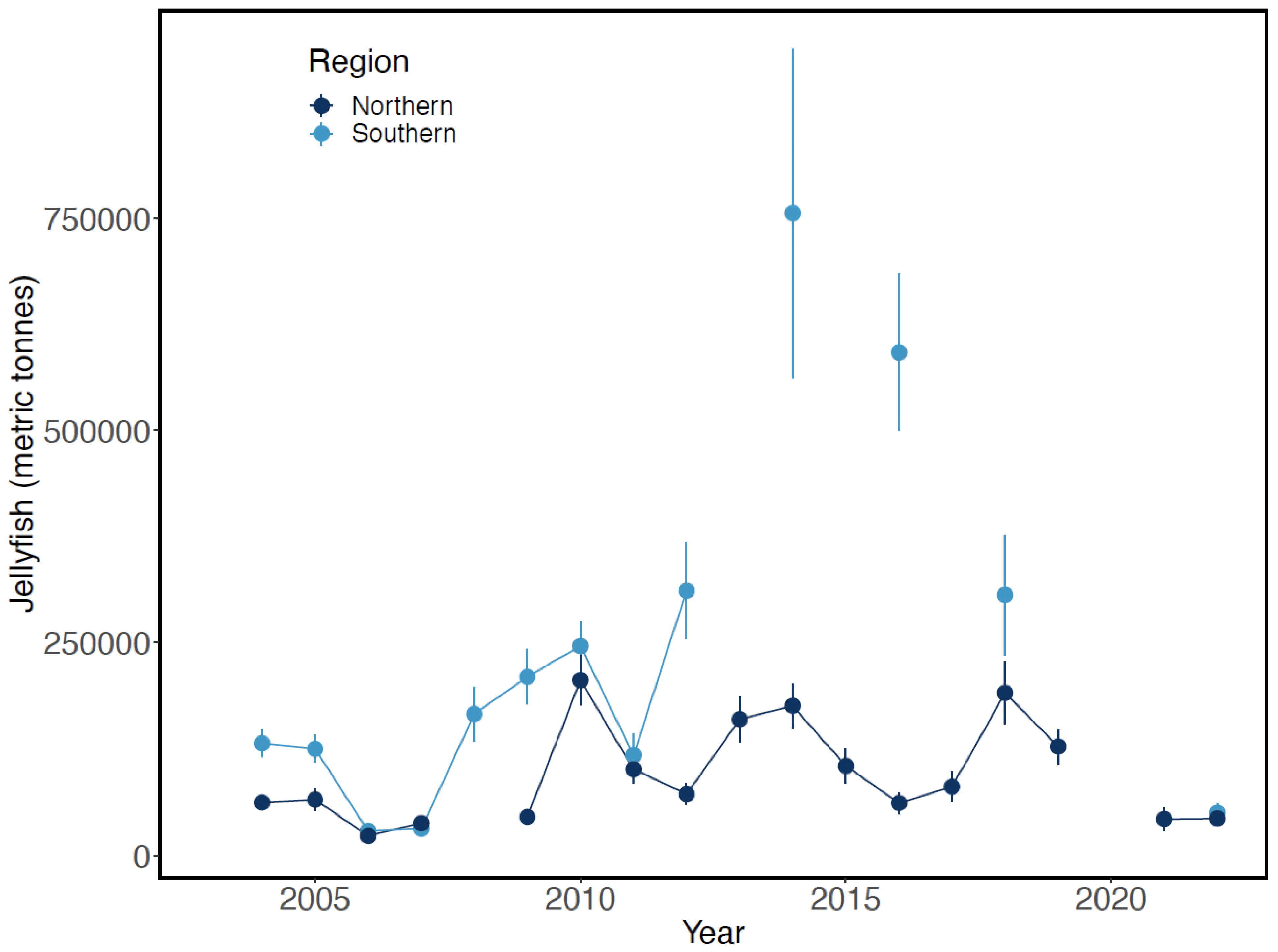
The abundance of small (<2 mm) and large (>2 mm) copepods, and euphausiids smaller than 15 mm has been estimated from 1998 to 2022 along the 70 m isobath in May within the middle domain (50–100 m depth) of the southeastern Bering Sea, and from 1996 to 2022 within the middle domain in August–September (Figure 17). Abundances of large copepods sampled in May were low from 2002 to 2006, a period of relatively warm temperatures and low sea ice cover (Figure 9 and Figure 11), then increased by factors of up to 100 during the subsequent colder years of 2007–2014 (Figure 17A). Abundances then declined after 2014 to numbers typical of the 2002–2006 period, with a rebound in 2017. By August–September, large copepods were generally abundant from 2000 to 2014 except for 2006, 2007, and 2013, with a generally declining trend after 2014 (Figure 17B). In contrast, a generally declining trend of small copepod abundances in the middle domain from 2004 to 2013 reversed after 2013 and remained elevated through at least 2020 (Figure 17). Additionally, euphausiid abundances were generally stable during these periods, apart from isolated peaks in May 2017 and August–September 2003.

4.3. Jellyfish

Late-summer biomass of jellyfish was exceptionally high in 2014 and 2016 in the upper 25 m layer in the southeastern Bering Sea, returning to pre-2014 levels by 2018 (Figure 18). These increases were not evident during the previous warm period of 2002–2006. In contrast, jellyfish biomass in the northern Bering Sea appeared unrelated to warm- or cold-water periods from 2004 to 2022. Jellyfish biomass was not estimated in the southeastern Bering Sea in 2020, in odd-numbered years between 2013 and 2021, or in the northeastern Bering Sea in 2008 and 2020.

4.4. Alaska Pollock and Pacific Cod

As the largest fishery by volume in the United States, Alaska pollock (Gadus chalcogrammus) in the eastern Bering Sea has been monitored intensively over the last 50 years. Pollock abundance is evaluated by one of the most advanced stock assessments available, which provides estimates of abundance-at-age dating from the mid-1960s (Ianelli et al., 2021) [39]. These results show that pollock recruitment is highly variable, with episodic high recruitment events every 4–5 years sustaining the population over time. The two lowest periods of recruitment to Age 1 juveniles since 1990, leading by one year, are first associated with the 2002–2006 period of warm SST and low sea ice cover, and second with the entry of The Blob into the eastern Bering Sea (Figure 19A). This association suggests that unusually warm surface waters may have contributed to the low recruitments during these two periods. Recruitment to Age 1 of Pacific cod (Gadus morhua) responded similarly to the 2002–2006 period of warm SST and low sea ice cover and to The Blob (Figure 19B). Pacific cod also support an important fishery in the eastern Bering Sea.

4.5. Pacific Halibut

Pacific halibut (Hippoglossus stenolepis) biomass in the eastern Bering Sea underwent two declines since 1994, both of which were associated with warmer water periods. The first of these declines persisted from 2000 to 2005, approximately contemporaneous with the 2002–2006 warm-water period, and the second began after 2015, following the entry of The Blob into the Bering Sea (Figure 20). These biomass estimates are based on the weight per unit effort of fish greater than 32 inches (81.6 cm) in fork length caught in fishery-independent setline surveys. The annual mean value of 7.91 lbs/skate in 2022 implies a decline by a factor of nearly three from the peak value of 21.4 lbs/skate in 2000.

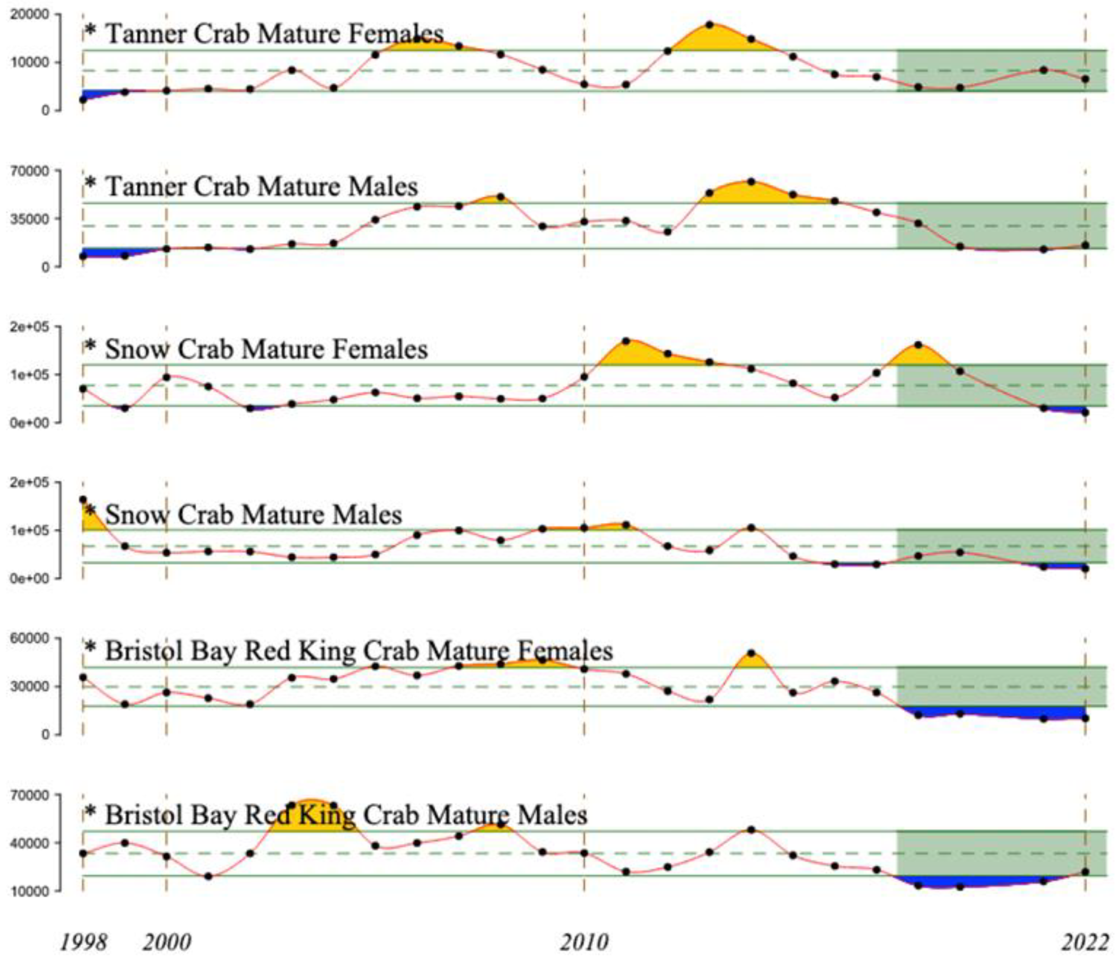
4.6. Red, Snow, and Tanner Crabs

Red, snow, and tanner crabs (Paralithodes camtschaticus, Chionoecetes opilio, and C. bairdi, respectively) have all supported major fisheries in the eastern Bering Sea and are all now in a state of decline (Figure 21). The decline in red king crabs began after 2014 and became severe after 2017. Declines of snow crab males also began after 2014, but females temporarily recovered after 2016 from a decline that began in 2011, reaching their most recent peak in 2018, followed by another decline through 2022. Tanner crabs declined from recent peaks in 2013 (females) or 2014 (males), with females recovering to the time-series mean by 2021.

4.7. Salmon

Responses of Pacific salmon to The Blob varied by species. The abundance of juvenile (age 2) Chinook salmon (Oncorhynchus tshawytscha) declined almost monotonically after 2015, but juvenile (ages 2–4) sockeye salmon (O. nerka) and juvenile pink salmon (O. gorbuscha) were relatively abundant during the 2002–2006 water period and after the arrival of The Blob in 2014 in the southeastern Bering Sea (Figure 22). In contrast, trends in the abundance of juvenile chum (O. keta) did not appear related to periods of relatively warm or cool waters in the eastern Bering Sea (Figure 68 in Murphy et al., 2022 [42]).

4.8. Seabirds

Reproductive success of five species of piscivorous seabirds on St. George and St. Paul Islands in the southeastern Bering Sea declined nearly in concert following The Blob’s arrival. These five species include common and thick-billed murres (Uria aalge and U. lomvia), black- and red-legged kittiwakes (Rissa tridactyla and R. brevirostris), and red-faced cormorants (Urile urile). Reproductive success of common and thick-billed murres on St. George Island, along with black- and red-legged kittiwakes, and red-faced cormorants on both St. George and St. Paul Islands, declined sharply in 2015, while that of common and thick-billed murres on St. Paul Island declined sharply in 2016 (Figure 23). Reproductive success of all these species recovered by 2019 on both islands.

4.9. Range Extensions

Warming bottom waters have led to northwestward expansions or shifts in the distribution of benthic and pelagic fish and shellfish, including commercially important species such as Alaska pollock, Pacific cod, king crab, and tanner crab (Landeira et al., 2018 [45], Thorson et al., 2019 [46], Baker, 2021 [26], Levine et al., 2023 [47]). The cold pool near-disappearance has a major implication for walleye pollock and Pacific cod because these species avoid the cool pool; therefore, they are now expected to colonize the newly available areas of the EBSS that were previously occupied by the cold pool. Baker (2021) [26] documented dramatic spatial shifts in two ecologically important Arctic gadids (polar cod and saffron cod) and two commercially important sub-Arctic gadids (walleye pollock and Pacific cod): while Arctic gadids responded negatively to the warm epoch in the EBSS, the sub-Arctic gadids responded positively to the same changes; moreover, the sub-Arctic gadids moved to the NBSS.

5. Discussion

The multiple anomalous responses among the taxa we surveyed above in our results section suggest that The Blob caused a major disruption of the marine food web in the eastern Bering Sea. These anomalous responses spanned at least four and probably more trophic levels. While the taxa we surveyed do not represent the entire marine food web, they do represent major components of the trophic levels they occupy. Considered individually, there are many factors that, alone or in combination, might account for the population-level responses of the taxa we surveyed. However, taken together, these responses appear to be broadly consistent with a decrease in primary production that consequently reduced the efficiency of energy transfer across trophic levels (i.e., trophic transfer efficiency, or TTF), resulting in declines in abundance, biomass, or reproductive success in higher trophic levels.

Evidence for the reduction in TTF following the entry of The Blob into the Bering Sea begins with the response of primary productivity. Satellite measurements of chlorophyll-a in spring reflect phytoplankton standing stocks, which, based on the reasonable assumption that zooplankton grazing on phytoplankton is negligible through the initial stages of the spring phytoplankton bloom, implies a corresponding intensity of phytoplankton production. Off-shelf chlorophyll-a measurements during spring were above average through 2014, with the 2014 measurements completed before The Blob entered the Bering Sea in June of that year. Subsequent off-shelf measurements have confirmed a general decline (Figure 16). These declines imply reduced primary productivity in the Bering Sea Green Belt, the most productive region of the eastern Bering Sea (Springer et al., 1996), which contributes to primary production on the outer continental shelf of the eastern Bering Sea through advection onto the shelf (Hunt et al., 2008). Considered in isolation, this is tenuous support for concluding that primary productivity in the eastern Bering Sea declined substantially following the entry of The Blob, but the simultaneous response of zooplankton lends additional support.

The concurrent declines of large copepods and increases of small copepods beginning in 2014 suggest lower primary productivity as production switched from an ice-algal dominated production scheme to one that is dominated by open-water production (Mueter et al., 2021 [12] and references therein). In any case, this transition lengthens the food chain by increasing the mean number of trophic transfers to higher trophic-level consumers such as fish and seabirds. Even slight shifts in TTE can lead to large reductions at higher trophic levels (e.g., Eddy et al., 2021 [48]). Such reductions are exacerbated by the increased biomass of jellyfish (Figure 18), which diverts additional energy from most higher-order consumers.

Reduced energy flow to higher-order consumers is reflected in the reduced recruitment to Age 1 of Alaska pollock and Pacific cod (Figure 19), declining biomass of Pacific halibut (Figure 20), declining abundance of red, snow, and tanner crabs and of juvenile Chinook salmon (Figure 21 and Figure 22), and reduced reproductive success of common and thick-billed murres on St. George Island, and of black- and red-legged kittiwakes, and red-faced cormorants (all piscivorous seabirds) on St. George and St. Paul Islands (Figure 23), following the entry of The Blob into the eastern Bering Sea. The delayed decline by one year of murres on St. Paul Island may reflect the reduced effects of The Blob near St. Paul Island in 2014 compared with those at St. George Island, the latter island being closer to the shelf break. Many, but not all, of these taxa had similar responses to the prior warm-water period of 2002–2006 in the eastern Bering Sea.

Not all of the higher-order consumer responses we surveyed declined. Juvenile sockeye salmon abundances increased considerably during warm years, especially after the entry of The Blob into the southeastern Bering Sea, when subsequent sockeye fishery yields nearly doubled compared with the long-term mean (see Figure 70 in Cunningham et al., 2022 [49]). This likely resulted from concurrent survival increases of Alaska pollock in their first year of life. Juvenile sockeye salmon consumed much higher proportions of age-0 Alaska pollock during the 2002–2006 warm period and after entry of The Blob into the Bering Sea than they did during the intervening cold period (Yasumiishi et al., 2019 [50], 2020 [51]). High consumption rates of age-0 Alaska pollock by pink and chum salmon, and by other forage fish during these warm periods (Yasumiishi et al., 2020 [51]) may account at least in part for the relatively high abundance of juvenile pink salmon (Figure 22), the absence of trends in juvenile chum salmon abundance, and the poor recruitment of Alaska pollock to Age 1 (Figure 19).

Entry of The Blob into the Bering Sea also appears to have affected spatial distributions of multiple taxa. Warming bottom waters have led to northwestward expansions or shifts in the distribution of benthic and pelagic fish and shellfish, including commercially important species such as Alaska pollock, Pacific cod, king crab, and tanner crab (Baker 2021 [26], Landeira et al., 2018 [45], Thorson et al., 2019 [46], Levine et al., 2023 [47]). The Blob’s entry into the Bering Sea also seems to contribute to the proliferation of toxic or otherwise noxious microalgae. The harmful algal blooms (HABs, such as those causing paralytic shellfish poisoning) appear more frequently and spread more widely throughout the eastern Bering Sea as SST rises (Natsuike et al., 2017 [52]).

The population- and community-level responses to The Blob we surveyed here for the eastern Bering Sea differ substantially from comparable responses in the Gulf of Alaska. The effects of The Blob in the Gulf of Alaska were more intense and persistent, and the population- and community-level responses differed markedly (Suryan et al., 2021 [9]). In the Gulf of Alaska, microzooplankton biomass decreased in spring but increased in fall, and large copepods increased in response to lower chlorophyll during The Blob years. In addition, capelin and herring (both forage fishes) declined in the Gulf of Alaska during The Blob years. Seabirds also declined in the Gulf of Alaska during The Blob years, as they did in the eastern Bering Sea. Differences in the responses of these taxa between the Gulf of Alaska and the eastern Bering Sea likely result at least in part from the differences in the ecological structure of these two marine ecosystems. Biological productivity in the Bering Sea is strongly affected by sea ice extent and phenology, whereas the Gulf of Alaska is ice-free. While fishery yields increased with warming in subpolar waters owing to the extension of the annual production cycle (Sherman et al., 2011 [53], 2013 [54]), it is not clear whether this effect will be more important than the loss of production associated with a loss of sea ice, which is occurring in the Bering Sea.

6. Conclusions

We reviewed various physical drivers and biological responses to the 2013–2015 marine heat wave in the Northeast Pacific. The anomaly dubbed “The Blob” emerged in 2013–2014 and persisted through 2015–2016, with some signs of its lingering through 2017–2018 and a possible return in 2019. A large salinity anomaly in the surface and subsurface layers preceded The Blob and contributed to its formation by enhancing stratification and trapping heat in the shallow mixed layer. The Blob’s successive appearances in the Northeast Pacific are suggestive of its advection by coastal currents around the Gulf of Alaska, along the Aleutians, and into the Bering Sea, where it was transported by the Bering Slope Current and shelf currents to the Bering Strait. During The Blob’s development in 2013–2014, advection along the Polar Front likely contributed to The Blob’s propagation to the Gulf of Alaska, along the Aleutians, and into the EBS. Owing to its extreme persistence and exceptional magnitude, The Blob and attendant physical changes impacted, sometimes dramatically, various aspects of the EBS ecosystem. A comparison of the time series of the population responses across trophic levels suggests that The Blob lowered primary production during spring, increased production of small copepods and jellyfish, and reduced the efficiency of energy transfer to higher trophic levels. The multi-year duration of The Blob likely preconditioned the EBS for the record-low seasonal sea ice extent and the disappearance of the cold pool in 2016 and 2018 that profoundly affected zooplankton, invertebrates, fishes, seabirds, and marine mammals. While the Bering Sea’s water temperature, seasonal sea ice, and cold pool seem to have returned to the long-term mean state in 2022, it remains to be seen whether the Bering Sea ecosystem will return to its previous state in the short term. Likely alternatives include either irreversible changes or hysteresis recovery.

References

1. Freeland, H. Something odd in the Gulf of Alaska. CMOS Bull. SCMO 2014, 42, 57–59. [Google Scholar]
2. Freeland, H. The “Blob” or Argo and other views of a large anomaly in the Gulf of Alaska in 2014/15. In State of the Physical, Biological and Selected Fishery Resources of Pacific in 2014; Canadian Technical Report of Fisheries and Aquatic Sciences; Chandler, P.C., King, S.A., Perry, R.I., Eds.; Fisheries & Oceans Canada Institute of Ocean Sciences: Sidney, BC, Canada, 2015; pp. 25–29. [Google Scholar]
3. Freeland, H.; Ross, T. ‘The Blob’—Or, how unusual were ocean temperatures in the Northeast Pacific during 2014–2018? Deep. Sea Res. Part I 2019, 150, 103061. [Google Scholar] [CrossRef]
4. Bond, N.A.; Cronin, M.F.; Freeland, H.; Mantua, N. Causes and impacts of the 2014 warm anomaly in the NE Pacific. Geophys. Res. Lett. 2015, 42, 3414–3420. [Google Scholar] [CrossRef]
5. Scannell, H.A.; Johnson, G.C.; Thompson, L.; Lyman, J.M.; Riser, S.C. Subsurface evolution and persistence of marine heatwaves in the Northeast Pacific. Geophys. Res. Lett. 2020, 47, e2020GL090548. [Google Scholar] [CrossRef]
6. Zhi, H.; Lin, P.F.; Zhang, R.H.; Chai, F.; Liu, H.L. Salinity effects on the 2014 warm “Blob” in the Northeast Pacific. Acta Oceanol. Sin. 2019, 38, 24–34. [Google Scholar] [CrossRef]
7. Holser, R.R.; Keates, T.R.; Costa, D.P.; Edwards, C.A. Extent and magnitude of subsurface anomalies during the Northeast Pacific Blob as measured by animal-borne sensors. J. Geophys. Res. Ocean. 2022, 127, e2021JC018356. [Google Scholar] [CrossRef]
8. Cavole, L.M.; Demko, A.M.; Diner, R.E.; Giddings, A.; Koester, I.; Pagniello, C.M.L.S.; Paulsen, M.L.; Ramirez-Valdez, A.; Schwenck, S.M.; Yen, N.K.; et al. Biological impacts of the 2013–2015 warm-water anomaly in the Northeast Pacific: Winners, losers, and the future. Oceanography 2016, 29, 273–285. [Google Scholar] [CrossRef] [Green Version]
9. Suryan, R.M.; Arimitsu, M.L.; Coletti, H.A.; Hopcroft, R.R.; Lindeberg, M.R.; Barbeaux, S.J.; Batten, S.D.; Burt, W.J.; Bishop, M.A.; Bodkin, J.L.; et al. Ecosystem response persists after a prolonged marine heatwave. Sci. Rep. 2021, 11, 6235. [Google Scholar] [CrossRef]
10. Schlitzer, R. Ocean Data View. 2022. Available online: https://odv.awi.de (accessed on 25 April 2023).
11. Belkin, I.M. Comparative assessment of the West Bering Sea and East Bering Sea Large Marine Ecosystems. Environ. Dev. 2016, 17, 145–156. [Google Scholar] [CrossRef]
12. Mueter, F.J.; Planque, B.; Hunt, G.L., Jr.; Alabia, I.D.; Hirawake, T.; Eisner, L.; Dalpadado, P.; Chierici, M.; Drinkwater, K.F.; Harada, N.; et al. Possible future scenarios in the gateways to the Arctic for Subarctic and Arctic marine systems: II. Prey resources, food webs, fish, and fisheries. ICES J. Mar. Sci. 2021, 78, 3017–3045. [Google Scholar] [CrossRef]
13. Ladd, C.; Eisner, L.B.; Salo, S.A.; Mordy, C.W.; Iglesias-Rodriguez, M.D. Spatial and temporal variability of coccolithophore blooms in the eastern Bering Sea. J. Geophys. Res. Ocean. 2018, 123, 9119–9136. [Google Scholar] [CrossRef]
14. Matson, P.G.; Washburn, L.; Fields, E.A.; Gotschalk, C.; Ladd, T.M.; Siegel, D.A.; Welch, Z.S.; Iglesias-Rodriguez, M.D. Formation, development, and propagation of a rare coastal coccolithophore bloom. J. Geophys. Res. Ocean. 2019, 124, 3298–3316. [Google Scholar] [CrossRef]
15. Peterson, W.; Bond, N.; Robert, M. The blob (part three): Going, going, gone? PICES Press 2016, 24, 46–48. [Google Scholar]
16. Zimmermann, M.; Prescott, M.M. Passes of the Aleutian Islands: First detailed description. Fish. Oceanogr. 2021, 30, 280–299. [Google Scholar] [CrossRef]
17. Belkin, I.M.; Krishfield, R.; Honjo, S. Decadal variability of the North Pacific Polar Front: Subsurface warming versus surface cooling. Geophys. Res. Lett. 2002, 29, 65.1–65.4. [Google Scholar] [CrossRef]
18. Belkin, I.M.; Shotwell, S.K. Advection of SST anomalies along the North Pacific Polar Front and their impact on the Gulf of Alaska, Aleutians, and Bering Sea ecosystems. In Proceedings of the Alaska Marine Science Symposium, Anchorage, AK, USA, 16–20 January 2012; p. 78, Alaska Marine Science Symposium Book of Abstracts, 2012. Available online: https://static1.squarespace.com/static/631a53939a3f0f445f25ea48/t/634f32a2155e8b13f868bba9/1666134698078/2012_AMSS_AbstractBook.pdf (accessed on 25 April 2023).
19. Shotwell, S.K.; Hanselman, D.H.; Belkin, I.M. Toward biophysical synergy: Investigating advection along the Polar Front to identify factors influencing Alaska sablefish recruitment. Deep. Sea Res. Part II 2014, 107, 40–53. [Google Scholar] [CrossRef]
20. Gentemann, C.L.; Fewings, M.R.; García-Reyes, M. Satellite sea surface temperatures along the West Coast of the United States during the 2014–2016 northeast Pacific marine heat wave. Geophys. Res. Lett. 2017, 44, 312–319. [Google Scholar] [CrossRef]
21. von Biela, V.R.; Arimitsu, M.L.; Piatt, J.F.; Heflin, B.; Schoen, S.K.; Trowbridge, J.L.; Clawson, C.M. Extreme reduction in nutritional value of a key forage fish during the Pacific marine heatwave of 2014−2016. Mar. Ecol. Prog. Ser. 2019, 613, 171–182. [Google Scholar] [CrossRef] [Green Version]
22. Walsh, J.E.; Thoman, R.L.; Bhatt, U.S.; Bieniek, P.A.; Brettschneider, B.; Brubaker, M.; Danielson, S.; Lader, R.; Fetterer, F.; Holderied, K.; et al. The high latitude marine heat wave of 2016 and its impacts on Alaska. Bull. Am. Meteorol. Soc. 2018, 99, S39–S43. [Google Scholar] [CrossRef]
23. Stabeno, P.J.; Danielson, S.L.; Kachel, D.G.; Kachel, N.B.; Mordy, C.W. Currents and transport on the Eastern Bering Sea shelf: An integration of over 20 years of data. Deep. Sea Res. Part II 2016, 134, 13–29. [Google Scholar] [CrossRef]
24. Thoman, R.L.; Bhatt, U.S.; Bieniek, P.A.; Brettschneider, B.R.; Brubaker, M.; Danielson, S.L.; Labe, Z.; Lader, R.; Meier, W.N.; Sheffield, G.; et al. The record low Bering Sea ice extent in 2018: Context, impacts, and an assessment of the role of anthropogenic climate change. Bull. Am. Meteorol. Soc. 2020, 101, S53–S58. [Google Scholar] [CrossRef] [Green Version]
25. Duffy-Anderson, J.T.; Stabeno, P.; Andrews, A.; Cieciel, K.; Deary, A.; Farley, E.; Fugate, C.; Harpold, C.; Heintz, R.; Kimmel, D.; et al. Responses of the northern Bering Sea and southeastern Bering Sea pelagic ecosystems following record-breaking low winter sea ice. Geophys. Res. Lett. 2019, 46, 9833–9842. [Google Scholar] [CrossRef] [Green Version]
26. Baker, M.R. Contrast of warm and cold phases in the Bering Sea to understand spatial distributions of Arctic and sub-Arctic gadids. Polar Biol. 2021, 44, 1083–1105. [Google Scholar] [CrossRef]
27. Thorson, J.T. Measuring the impact of oceanographic indices on species distribution shifts: The spatially varying effect of cold-pool extent in the eastern Bering Sea. Limnol. Oceanogr. 2019, 64, 2632–2645. [Google Scholar] [CrossRef]
28. Johnson, J.J.; Miksis-Olds, J.L.; Lippmann, T.C.; Jech, J.M.; Seger, K.D.; Pringle, J.M.; Linder, E. Decadal community structure shifts with cold pool variability in the eastern Bering Sea shelf. J. Acoust. Soc. Am. 2022, 152, 201–213. [Google Scholar] [CrossRef]
29. Danielson, S.L.; Ahkinga, O.; Ashjian, C.; Basyuk, E.; Cooper, L.W.; Eisner, L.; Farley, E.; Iken, K.B.; Grebmeier, J.M.; Juranek, L.; et al. Manifestation and consequences of warming and altered heat fluxes over the Bering and Chukchi Sea continental shelves. Deep. Sea Res. Part II 2020, 177, 104781. [Google Scholar] [CrossRef]
30. Stabeno, P.J.; Duffy-Anderson, J.T.; Eisner, L.B.; Farley, E.V.; Heintz, R.A.; Mordy, C.W. Return of warm conditions in the southeastern Bering Sea: Physics to fluorescence. PLoS ONE 2017, 12, e0185464. [Google Scholar] [CrossRef] [Green Version]
31. Stabeno, P.J.; Bell, S.W. Extreme conditions in the Bering Sea (2017–2018): Record-breaking low sea-ice extent. Geophys. Res. Lett. 2019, 46, 8952–8959. [Google Scholar] [CrossRef]
32. Belkin, I.M.; Cornillon, P.C. Bering Sea thermal fronts from Pathfinder data: Seasonal and interannual variability. Pac. Oceanogr. 2005, 3, 6–20. [Google Scholar]
33. Hunt, G.L., Jr.; Stabeno, P.J.; Strom, S.; Napp, J.M. Patterns of spatial and temporal variation in the marine ecosystem of the southeastern Bering Sea, with special reference to the Pribilof Domain. Deep. Sea Res. Part II 2008, 55, 1919–1944. [Google Scholar] [CrossRef]
34. Siddon, E. (Ed.) Ecosystem Status Report 2022: Eastern Bering Sea, Stock Assessment and Fishery Evaluation Report; North Pacific Fishery Management Council: Anchorage, AK, USA, 2022. [Google Scholar]
35. Nielsen, J.M.; Eisner, L.; Watson, J.; Gann, J.C.; Callahan, M.W.; Mordy, C.W.; Bell, S.W.; Stabeno, P. Spring satellite chlorophyll-a concentrations in the eastern Bering Sea. In Ecosystem Status Report 2022: Eastern Bering Sea, Stock Assessment and Fishery Evaluation Report; Elizabeth, S., Ed.; North Pacific Fishery Management Council: Anchorage, AK, USA, 2022; pp. 68–72. [Google Scholar]
36. Springer, A.M.; McRoy, C.P.; Flint, M.V. The Bering Sea Green Belt: Shelf-edge processes and ecosystem production. Fish. Oceanogr. 1996, 5, 205–223. [Google Scholar] [CrossRef]
37. Kimmel, D.; Barrett, J.; Cooper, D.; Crouser, D.; Deary, A.; Eisner, L.; Lamb, J.; Murphy, J.; Pinger, C.; Cormack, B.; et al. Current and historical trends for zooplankton in the Bering Sea. In Ecosystem Status Report 2022: Eastern Bering Sea, Stock Assessment and Fishery Evaluation Report; Elizabeth, S., Ed.; North Pacific Fishery Management Council: Anchorage, AK, USA, 2022; pp. 79–90. [Google Scholar]
38. Yasumiishi, E.; Andrews, A.; Murphy, J.; Dimond, A.; Farley, E.; Siddon, E. Trends in the biomass of jellyfish in the southeastern and northeastern Bering Sea during the late-summer surface trawl survey, 2003–2022. In Ecosystem Status Report 2022: Eastern Bering Sea, Stock Assessment and Fishery Evaluation Report; Elizabeth, S., Ed.; North Pacific Fishery Management Council: Anchorage, AK, USA, 2022; pp. 94–95. [Google Scholar]
39. Ianelli, J.; Fissel, B.; Stienessen, S.; Honkalehto, T.; Siddon, E.; Allen-Akselrud, C. Chapter 1: Assessment of the Walleye Pollock Stock in the Eastern Bering Sea. In Stock Assessment and Fishery Evaluation Report for the Groundfish Resources of the Bering Sea/Aleutian Islands Regions; Alaska Fisheries Science Center, National Marine Fisheries Service, National Oceanic and Atmospheric Administration: Seattle, WA, USA, 2021; p. 171. [Google Scholar]
40. Thompson, G.G.; Barbeaux, S.; Conner, J.; Fissel, B.; Hurst, T.; Laurel, B.; O’Leary, C.A.; Rogers, L.; Shotwell, S.K.; Siddon, E.; et al. Assessment of the Pacific Cod Stock in the Eastern Bering Sea. In NPFMC Bering Sea and Aleutian Islands SAFE; North Pacific Fishery Management Council: Anchorage, AK, USA, 2021; p. 494. [Google Scholar]
41. Richar, J. Eastern Bering Sea commercial crab stock biomass. In Ecosystem Status Report 2022: Eastern Bering Sea, Stock Assessment and Fishery Evaluation Report; Elizabeth, S., Ed.; North Pacific Fishery Management Council: Anchorage, AK, USA, 2022; pp. 140–141. [Google Scholar]
42. Murphy, J.; Garcia, S.; Cooper, D.; Farley, E.; Lee, E.; Dimond, A.; Howard, K. Northern Bering Sea juvenile salmon abundance indices. In Ecosystem Status Report 2022: Eastern Bering Sea, Stock Assessment and Fishery Evaluation Report; Elizabeth, S., Ed.; North Pacific Fishery Management Council: Anchorage, AK, USA, 2022; pp. 106–108. [Google Scholar]
43. Andrews, A.; Yasumiishi, E.; Farley, E.; Murphy, J.; Dimond, A. Trends in the abundance of juvenile sockeye salmon in the southeastern Bering Sea during the late-summer surface trawl survey, 2003–2020. In Ecosystem Status Report 2022: Eastern Bering Sea, Stock Assessment and Fishery Evaluation Report; Elizabeth, S., Ed.; North Pacific Fishery Management Council: Anchorage, AK, USA, 2022; pp. 105–106. [Google Scholar]
44. Akiya, A.; Ahkinga, S.; Divine, L.; Jones, T.; Kingeekuk, L.; Lestenkof, A.; Lindsey, J.; Niksik, T.; Padula, V.; Pungowiyi, P.; et al. Integrated seabird information. In Ecosystem Status Report 2022: Eastern Bering Sea, Stock Assessment and Fishery Evaluation Report; Elizabeth, S., Ed.; North Pacific Fishery Management Council: Anchorage, AK, USA, 2022; pp. 142–148. [Google Scholar]
45. Landeira, J.M.; Matsuno, K.; Tanaka, Y.; Yamaguchi, A. First record of the larvae of tanner crab Chionoecetes bairdi in the Chukchi Sea: A future northward expansion in the Arctic? Polar Sci. 2018, 16, 86–89. [Google Scholar] [CrossRef]
46. Thorson, J.T.; Fossheim, M.; Mueter, F.J.; Olsen, E.; Lauth, R.R.; Primicerio, R.; Husson, B.; Marsh, J.; Dolgov, A.; Zador, S.G. Comparison of near-bottom fish densities show rapid community and population shifts in Bering and Barents seas. In Arctic Report Card; Richter-Menge, J., Druckenmiller, M.L., Jeffries, M., Eds.; NOAA: Washington, DC, USA, 2019; pp. 72–80. [Google Scholar]
47. Levine, R.M.; De Robertis, A.; Grünbaum, D.; Wildes, S.; Farley, E.V.; Stabeno, P.J.; Wilson, C.D. Climate-driven shifts in pelagic fish distributions in a rapidly changing Pacific Arctic. Deep. Sea Res. Part II 2023, 208, 105244. [Google Scholar] [CrossRef]
48. Eddy, T.D.; Bernhardt, J.R.; Blanchard, J.L.; Cheung, W.W.L.; Colléter, M.; du Pontavice, H.; Fulton, E.A.; Gascuel, D.; Kearney, K.A.; Petrik, C.M.; et al. Energy flow through marine ecosystems: Confronting transfer efficiency. Trends Ecol. Evol. 2021, 36, 76–86. [Google Scholar] [CrossRef]
49. Cunningham, C.J.; Vega, S.; Head, J. Temporal trend in the annual inshore run size of Bristol Bay sockeye salmon (Oncorhynchus nerka). In Ecosystem Status Report 2022: Eastern Bering Sea, Stock Assessment and Fishery Evaluation Report; Elizabeth, S., Ed.; North Pacific Fishery Management Council: Anchorage, AK, USA, 2022; pp. 109–110. [Google Scholar]
50. Yasumiishi, E.; Cunningham, C.; Farley, K.C.; Moss, J.; Strasburger, W.; Eisner, L.; Andrews, A.; Gann, J.; Murphy, J.; Dimond, A.; et al. Mechanisms for shifts in the distribution and abundance of juvenile sockeye salmon in the Eastern Bering Sea during late summer, 2002–2018. In North Pacific Anadromous Fish Commission Technical Report No. 15; North Pacific Fishery Management Council: Anchorage, AK, USA, 2019; pp. 129–131. [Google Scholar]
51. Yasumiishi, E.M.; Cieciel, K.; Andrews, A.G.; Murphy, J.; Dimond, J.A. Climate-related changes in the biomass and distribution of small pelagic fishes in the eastern Bering Sea during late summer, 2002–2018. Deep. Sea Res. Part II 2020, 181–182, 104907. [Google Scholar] [CrossRef]
52. Natsuike, M.; Saito, R.; Fujiwara, A.; Matsuno, K.; Yamaguchi, A.; Shiga, N.; Hirawake, T.; Kikuchi, T.; Nishino, S.; Imai, I. Evidence of increased toxic Alexandrium tamarense dinoflagellate blooms in the eastern Bering Sea in the summers of 2004 and 2005. PLoS ONE 2017, 12, e0188565. [Google Scholar] [CrossRef] [Green Version]
53. Sherman, K.; O’Reilly, J.; Belkin, I.M.; Melrose, C.; Friedland, K.D. The application of satellite remote sensing for assessing productivity in relation to fisheries yields of the world’s large marine ecosystems. ICES J. Mar. Sci. 2011, 68, 667–676. [Google Scholar] [CrossRef] [Green Version]
54. Sherman, K.; Belkin, I.M.; Friedland, K.D.; O’Reilly, J. Changing states of North Atlantic large marine ecosystems. Environ. Dev. 2013, 7, 46–58. [Google Scholar] [CrossRef]
Figure 1. January 2014 SST departure (in standard deviations) from the 1981–2013 Reynolds NCEP. dataset. Adapted from Freeland (2014, Figure 2) with permission from the author.
Jmse 11 00958 g001
Figure 2. SST anomalies (in standard deviations) for October 2013 (top), March 2014 (middle), and September 2014 (bottom). The solid blue line is “Line P”, an oceanic transect from Vancouver Island to Ocean Station Papa. Adapted from Freeland (2015) ([2], Figure 6-1) with permission.
Jmse 11 00958 g002
Figure 3. The temperature anomaly (in standard deviations) at Ocean Station Papa from data interpolated to that location from Argo floats. The mean state and distribution of standard deviation vary with depth and time of year. The average distribution of the standard deviation with depth is shown to the right of the contour plot. Adapted from Freeland and Ross (2019) ([3], Figure 5) with permission.
Jmse 11 00958 g003
Figure 4. Surface circulation of the Bering Sea (schematically). Main currents: AC, Anadyr Current; ACC, Alaska Coastal Current; ANSC, Aleutian North Slope Current; AS, Alaskan Stream; BSC, Bering Slope Current; EKC, East Kamchatka Current. Aleutian passes and straits, east-to-west (downstream): U, Unimak Pass; Amu, Amukta Pass; Amc, Amchitka Pass; B, Buldir Pass; N, Near Strait; K, Kamchatka Strait. The base map was created with the Ocean Data View (ODV) software developed by Schlitzer (2022) [10]. Reproduced from Belkin (2016) ([11], Figure 3).
Jmse 11 00958 g004
Figure 5. Polar Front crossings (circles) and long-term mean path (white line). Arrows are the Alaskan Stream’s branches into the Bering Sea. Reproduced after Belkin et al. (2002) ([17], Figure 1).
Jmse 11 00958 g005
Figure 6. Monthly SST anomalies in Prince William Sound, Alaska. Dashed lines indicate timing (July) of biological collections in 2012–2016. Adapted from von Biela et al. (2019) ([21], Figure 3). The most abrupt warming of the entire record in June 2013 likely signaled the arrival of the leading edge of The Blob advected by the Alaska Coastal Current.
Jmse 11 00958 g006
Figure 7. Top: Map showing the location of the Seward Line and GAK1 station. Bottom: Monthly water temperature anomalies in the 0–50 m layer. Source: http://research.cfos.uaf.edu/gak1/ (accessed on 25 April 2023). The Blob’s crossing of the Seward Line in mid-2013 is consistent with The Blob’s arrival in Prince William Sound in June 2013 (Figure 6).
Jmse 11 00958 g007
Figure 8. January–December 2016 ocean heat content anomaly (°C) from the surface to 300 m or bottom of ocean column. Reproduced from Walsh et al. (2018) ([22], Figure 8.1) with permission.
Jmse 11 00958 g008
Figure 9. Average sea ice extent in the Bering Sea in January–April. Reproduced from Thoman et al. (2020) ([24], Figure 1a).
Jmse 11 00958 g009
Figure 10. Maximum (2012) and minimum (2018) annual sea ice extent. Reproduced from Duffy-Anderson et al. (2019) ([25], Figure 1) with permission. M2, M4, M5, and M8 are moorings.
Jmse 11 00958 g010
Figure 11. Annual mean anomalies of bottom temperature (left) and SST (right) in the NOAA−EBSS area. Reproduced from Baker (2021) ([26], Figure 4) with permission.
Jmse 11 00958 g011
Figure 12. Maps of SST (left) and bottom temperature (right) based on data from NOAA EBSS and NBSS bottom trawl surveys in 2010 (top), 2017 (middle), and 2018 (bottom). Reproduced from Baker (2021) ([26], Figure 3) with permission.
Jmse 11 00958 g012
Figure 13. Maps of bottom temperature on the EBSS. Reproduced from Thorson (2019) ([27], Figure 1).
Jmse 11 00958 g013
Figure 14. Summer bottom temperatures in the NBS and SEBS in 2018 (color ramp); spring–autumn sampling stations during 2018 (dots). Adapted from Duffy-Anderson et al. (2019) ([25], Figure 1b) with permission.
Jmse 11 00958 g014
Figure 15. Top: Seasonal paths of SST fronts, May–November 1985–1996. Bottom: Long-term mean frequency of SST fronts in November 1985–1996. Reproduced from Belkin (2016) ([11], Figure 4). Original maps are from Belkin and Cornillon (2005) [32].
Jmse 11 00958 g015
Figure 16. (A) Map of 8 shelf regions used for satellite chlorophyll-a monitoring. Off-shelf denotes regions on the shelf break and slope deeper than 200 m. (B) Average spring (April–June) chlorophyll-a concentrations. Black dotted line denotes the long-term median for each region. Dark-blue bars indicate data for the year 2022. Adapted from Figures 39 and 40 in Nielsen et al. (2022) [35].
Jmse 11 00958 g016
Figure 17. Abundance of large (>2 mm) and small (<2 mm) copepods and euphausiids (<15 mm) sampled in the southeastern Bering Sea in (A) May, along the 70 m isobath, and (B) August–September, within the middle shelf (50–100 m depth), as part of the Bering Arctic Sub-arctic Integrated Survey (BASIS). Black circles denote estimates from sample enumerations in the laboratory, and blue triangles denote preliminary results from rapid zooplankton assessments (RZA) aboard ships. Note logarithmic scales for large and small copepods. Adapted from Figures 48 and 51 in Kimmel et al. (2022) [37].
Jmse 11 00958 g017
Figure 18. Estimated biomass of jellyfish in the upper 25 m layer in the eastern Bering Sea during late summer, 2004–2022. Adapted from Figure 58 in Yasumiishi et al. (2022) [38].
Jmse 11 00958 g018
Figure 19. Estimated recruitment of (A) Alaska pollock and (B) Pacific cod to Age 1 in the eastern Bering Sea, based on data presented, respectively, in Tables 1–28 in Ianelli et al. (2021) [39] and Table 2.11a in Thompson et al. (2021) [40].
Jmse 11 00958 g019
Figure 20. Mean weight per unit effort over-32 inch-length Pacific halibut caught during the International Pacific Halibut Commission’s Fishery-Independent Setline Surveys in area 4CDE of the eastern Bering Sea, 1993–2022. Shaded area indicates 95% credibility intervals. Data retrieved from http://iphc-shiny2.westus.cloudapp.azure.com:3838/IPHC_ShinyApps/SpaceTimeExplorer/ (accessed on 25 April 2023).
Jmse 11 00958 g020
Figure 21. Abundance estimates of red, snow, and tanner crabs in the eastern Bering Sea, 1998–2022. Dashed and solid green lines indicate the mean and ±1 standard deviation for the time series, and orange and blue indicate deviations greater than one standard deviation from the mean. Green shading indicates the most recent 5 years. Adapted from Figure 92 in Richar (2022) [41].
Jmse 11 00958 g021
Figure 22. Abundance estimates of (A) juvenile Chinook salmon in the northern Bering Sea (NBS), 2003–2022, (B) juvenile sockeye salmon in the northern and southern Bering Sea, and (C) juvenile pink salmon in the northern Bering Sea. Juvenile Chinook salmon are typically in their second year of life, juvenile sockeye salmon may be in their second through fourth years of life, and juvenile pink salmon are in their first year of life. Adapted from Figures 67 and 69 in Murphy et al. (2022) [42], and Figure 66 in Andrews et al. (2022) [43].
Jmse 11 00958 g022
Figure 23. Reproductive success of five species of piscivorous seabirds on St. Paul and St. George Islands in the EBS, 1996–2022. Green lines indicate the mean and ±1 standard deviation. Orange and blue shadings indicate deviations greater than one standard deviation from the mean. Green shading indicates the most recent 5 years. Adapted from Figure 93 in Akiya et al. (2022) [44].
Jmse 11 00958 g023
Disclaimer/Publisher’s Note: The statements, opinions and data contained in all publications are solely those of the individual author(s) and contributor(s) and not of MDPI and/or the editor(s). MDPI and/or the editor(s) disclaim responsibility for any injury to people or property resulting from any ideas, methods, instructions or products referred to in the content.