Article

Disentangling Population Level Differences in Juvenile Migration Phenology for Three Species of Salmon on the Yukon River

by
Katharine B. Miller
1,* and
Courtney M. Weiss
2
1
National Oceanic and Atmospheric Administration, National Marine Fisheries Service, Alaska Fisheries Science Center, 17109 Point Lena, Loop Road, Juneau, AK 99801, USA
2
Yukon Delta Fisheries Development Association, 2909 Arctic Blvd., Anchorage, AK 99503, USA
*
Author to whom correspondence should be addressed.
J. Mar. Sci. Eng. 2023, 11(3), 589; https://doi.org/10.3390/jmse11030589
Submission received: 1 February 2023 / Revised: 6 March 2023 / Accepted: 7 March 2023 / Published: 10 March 2023
(This article belongs to the Special Issue Ecosystem-Based Fishery Management in the Bering Sea)

Abstract

:
Migration phenology influences many important ecological processes. For juvenile Pacific salmon, the timing of the seaward migration from fresh to marine waters is linked to early marine survival and adult returns. Seaward migration phenology is determined by interactions between the intrinsic attributes of individual species and environmental factors that are acting upon them. Temperature and discharge are two factors of the freshwater environment that have been shown to influence intra- and interannual variation in juvenile salmon phenology, but these factors may affect the migrations of sympatric species differently. Understanding how variations in phenology change with environmental heterogeneity is a critical first step in evaluating how the future climate may affect salmon. This is especially crucial for high-latitude rivers, where the pace of climate change is nearly twice as rapid as it is for more temperate areas. This research investigates the influence of river conditions on the seaward migration phenology of Chinook, chum, and coho salmon in the Yukon River. The results identified species-specific differences in the factors affecting migration duration, concentration, and skew and provide a starting point for a more detailed examination of how phenological variability may affect the temporal matching of juvenile salmon with biological resources and environmental conditions for optimal survival.

1. Introduction

Pacific salmon have been an important means of subsistence and cultural resource for the Yukon River area for millennia. In the recent past, they have also supported robust commercial fisheries that provided employment in remote locations with limited economic opportunities. Chinook salmon (Oncorhynchus tshawytscha) have been in a prolonged period of low productivity since the early 1990s, resulting in the complete closure of commercial and subsistence fisheries in 2011 and 2020, respectively. Chum salmon (Oncorhynchus keta) and coho salmon (Oncorhynchus kisutch) suffered catastrophic declines in adult returns beginning in 2021 and have been closed to commercial and subsistence fishing since. The role of freshwater versus marine factors in these declines is unclear. Substantial effort has been invested in understanding the factors contributing to the survival and recruitment of Chinook salmon once they enter the marine environment [1,2]. In the Northern Bering Sea (NBS), research on juvenile Yukon River Chinook salmon at the end of the first marine summer identified a positive correlation between the abundance of Canadian-origin juvenile salmon in the NBS and adult returns to the Yukon River [3]. This relationship suggests that factors affecting recruitment likely occur earlier in the salmon life cycle.
The migration from freshwater to the marine environment is a critical life-history threshold for juvenile salmon, requiring changes in morphology, physiology, and behavior in response to environmental cues. Migration phenologies have evolved to exploit natural variations in local abiotic conditions and resource pulses that favor survival and growth. A substantial body of research on juvenile salmon indicates that the onset of seaward migration is linked to environmental conditions (see [4,5,6,7,8]). The timing of seaward migration has been linked with early marine survival and the subsequent return to spawn as adults. Survival is higher when migration coincides with optimal ocean prey and environmental conditions [9]. Seaward migration phenology is a population-level process that can vary between co-occurring salmonid species [7] as species with different life histories respond to the same environmental factors in different ways. Very few studies have examined synchrony in the downstream migration between sympatric species [10,11]. A better understanding of this phenological synchrony could identify whether relationships between migration timing and hydrology vary across species, which hydrologic factors are most important in determining seaward migration phenology for each species and enhance understanding of how natural and climate-induced environmental changes may alter migration patterns in the future.
The environmental factors affecting the downstream migration of anadromous species have been investigated by a number of researchers (see [10,12]). Some evidence suggests that water temperature and discharge are important factors in determining the timing, rate, and duration of migration [13,14,15], while other studies have found little to no relationship with these factors [16]. Many of the studies evaluating the role of both temperature and discharge have focused on small rivers [17] or highly altered systems with controlled flow regimes [18,19], and as such, may not be applicable to large natural rivers, particularly those in high latitudes with strong seasonal temperature extremes. Climate change is having a pronounced effect on arctic ecosystems. Over the last 60 years, climate warming in Alaska has been almost twice as rapid as in the rest of the United States [20], impacting both marine and freshwater systems important to Pacific salmon. Climate-induced impacts on northern freshwater systems can cause disruptions to the hydrological cycle [21] and the complex interactions between temperature, ice, precipitation, and permafrost. These changes are expected to affect river discharge and temperature during juvenile salmon rearing and seaward migration, with the potential to disrupt seaward migration cycles.
This research investigates the influence of river conditions on the seaward migration phenology of Chinook, chum, and coho salmon in a large, subarctic river. The primary objectives of the research are to evaluate synchrony in emigration timing and the shape of the migration phenology distributions between these sympatric species and to identify environmental covariates that may influence these differences.

2. Materials and Methods
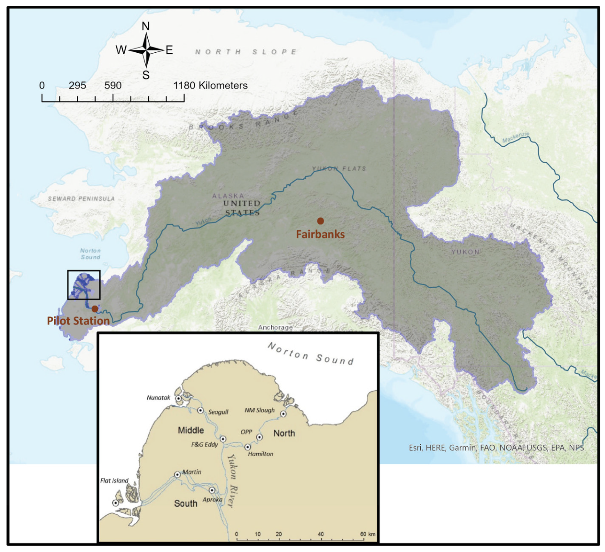
2.1. Study Area

The Yukon River, located in northwest Canada and central Alaska, is the fourth-largest river in North America and one of its largest and most diverse intact ecosystems [22]. The Yukon River watershed encompasses over 832,000 km2 (Figure 1) and is divided into 13 major hydrologic basins [22,23], all of which are underlain by varying amounts of permafrost [24]. The river is fed by eight major tributaries and numerous distributaries. Below St. Mary’s, approximately 168 miles upstream from the southern river mouth, the Yukon splits into three primary distributaries, each discharging into the Bering Sea. These distributaries flow across the Yukon River Delta, a gently sloping subarctic coastal plain, and across the submerged delta platform that extends 10–30 km offshore. Free-floating and landfast ice occur over the delta platform and along the delta shoreline seasonally from late fall through early spring [25]. Sub-ice channels extend from major distributaries, transporting Yukon River flow offshore during ice-covered periods [26].
Yukon River hydrology changes seasonally. For a six-to-nine-month period, the region is snow-covered with minimal streamflow. Peak discharges occur concurrent with or shortly after river breakup in the early spring, and high river flow continues until ice-up in late fall. In the lower river, discharge ranges from as low as 1200 m3 s−1 in winter to a springtime peak in excess of 19,800 m3 s−1 [27]. The spring discharge pulse is primarily driven by snow melt [23,28], with additional contributions from glacial ice melt, precipitation, and melting permafrost [29,30,31]. The relationship between accumulated snow (snowpack), snow melt, and river ice breakup is complex [23,28]. As temperatures rise in the spring, the snowpack undergoes a period of melting and refreezing as the snowpack becomes fully saturated with water. This period is known as the “snow melt duration” [28] and is followed by the snow off date, which is the last day of significant snow cover [23] and a period of reduced surface albedo and enhanced solar energy loading [32]. Snow off and the onset of snow melt are correlated with the timing of river breakup and discharge and snow off is also correlated to spring air temperatures across much of the Yukon basin [23]. The timing of the highest river discharge coincides with the start of annual migrations of juvenile salmon from the river to the Bering Sea; however, the extent to which earlier hydrological processes, such as the snow melt duration, affect seaward migration timing is unknown.
Chinook, chum, and coho salmon have different life history characteristics. Chinook and chum salmon spawn along the river and its tributaries up to the headwaters, over 3000 km from the coast [33]. Coho salmon spawning locations are not well documented, but they are believed to spawn throughout the lower river into the Tanana River, but not past the Yukon River’s boundary with Canada [34]. Chinook salmon are composed of 36 spatially and genetically distinct populations with similar timings for adult spawning migrations [35]. Chum salmon can be genetically assigned to two populations: summer and fall [36]. Summer chum adults enter the river in June and spawn predominantly in the lower river, while fall chum adults enter the river in July and spawn higher in the watershed into Canada. Juvenile Chinook salmon spend a year rearing in freshwater before migrating but may move downstream from the spawning areas during this rearing period [37,38]. Juvenile chum salmon migrate to the ocean shortly after hatching from the locations where they were spawned, but Chinook spend a year rearing in freshwater before emigrating. Juvenile coho generally spend one to three years rearing in freshwater before migrating to the ocean and may move considerably during this time.

2.2. Biological Data

Since 2014, salmon and other juvenile fish species have been captured at nine permanent stations on the three main distributaries of the lower Yukon River (Figure 1) near the village of Emmonak. Stations were sampled three times per week from ice-out from the middle of May through the end of July using surface tow nets (6.8 m long × 1.8 m2 at the mouth, tapering to a 0.3 m × 0.3 m cod end). Few juvenile salmon are captured after the end of July, and it is difficult to know whether these salmon are emigrating or relocating to winter nursery areas farther downstream. Therefore, the end of July was selected as the end of the migration. At each station, three replicate 15-min tows were performed during daylight hours by two small (i.e., 6 to 7 m) open skiffs towing against the current and holding the net open. Surface temperature measurements were taken at the start of sampling at each station. At the end of each tow, captured fish were sorted into species. All juvenile Chinook and coho salmon were retained for further analysis, while individuals of other species, including chum salmon, were enumerated, measured, and released. Retained salmon were placed in refrigerated bait coolers by station and transported alive to the field station in Emmonak. At the field station, salmon were photographed, euthanized, measured to 1 mm fork length, weighed to 0.001 g, and frozen. The caudal fin was clipped and placed in ethanol for genetic stock identification. The frozen samples were transported to the National Oceanic and Atmospheric Administration’s (NOAA) laboratory in Juneau, Alaska.

2.3. Phenology Modeling

Seaward migration phenology in juvenile salmon can be thought of as a series of migration completions carried out by individuals in a population over time. While phenology is typically evaluated using discrete events, such as the onset, mid-point, and end of the migration (generally determined to be 5%, 50%, and 90–95% of the total run, respectively) [39,40], this approach loses information on the shape of the migration distribution throughout its duration [39,41,42]. These methods do not easily lend themselves to the comparison of phenological phenomena between species because they lack common model parameters to evaluate against environmental variables. Parameters, such as the time required to complete the migration, the spread of individuals over the migration duration, and the skew of the distribution, are all variables that can be affected by the migration environment and by changes in that environment over time. Phenology distributions are often leptokurtic or skewed, and their shapes may change from year to year. These factors limit the applicability of measures of central tendency such as the median and the mean [42,43,44] for comparing differences in phenology between species and time periods. Recognizing these limitations, analytical methods that consider the full phenological distribution have been developed to more accurately compare the overlap or gaps between the distributions of sympatric species or the same species over time (see [42,44,45,46,47,48,49]). In this research, migration is modeled in terms of cumulative probabilities, making it possible to compare migrations of different durations and numbers of individuals. The model parameters describe important characteristics of the phenology distribution that can be used to compare models to one another and to environmental covariates.
The biological dataset used for this research comprised daily totals of Chinook, chum, and coho salmon smolts intercepted at the sampling stations for the periods 2014–2019 and 2021. In 2020, the start of sampling was delayed by two weeks because of the COVID-19 pandemic. Since the juvenile salmon emigration was underway by the time sampling started, these data were not included in this analysis. Daily totals for a given sampling day were pooled across all stations sampled that day. The study was designed for the effort to remain constant across years, but some differences in effort occurred due to equipment malfunctions and weather delays. To address this, catch per unit effort (CPUE) for each sampling day was calculated as the total catch divided by the number of tows. The use of CPUE instead of total count made no appreciable difference to the models, so the total count was selected for use due to its easier interpretability.
Daily catches of Chinook, chum, and coho salmon were modeled for each year as the cumulative probability of migration using the inverse logit, as modified by Franco [43]:
y y m a x = 1 ( 1 r m a x 1 + e c x t ) x
Using proportions as the response makes this model robust to sample size differences between years and species. Parameter rmax, the maximum proportional rate of migration completion, is a dimensionless variable that describes the rate at which the cumulative distribution function (cdf) increases to its maximum value. In this study, all intercepted salmon were defined as successful migrations, and the end of the sampling period was the end of July. Very small numbers of juvenile salmon are captured close to or at the end of the sampling period. As a result, in this analysis, rmax is nearly equivalent to the length of the sampling period. Parameter c is a measure of the concentration or spread of the distribution (units: time−1); increasing values of c reduce the spread of the probability density function (pdf). Parameter t is a weighted measure of the migration duration.
The start of migration was defined as the number of days from the official ice breakup date in Emmonak, which changed each year [50]. Breakup date was chosen over “day of year” because field sampling indicates that the bulk of the migration for the species being evaluated occurs after ice leaves the river [51,52]. The objective of the research was to compare seaward migration phenologies between salmon species during the period in which that migration can occur each year. The day of the year on which migration becomes possible is determined by the ice breakup date; therefore, the day of year by itself has limited value in this analysis.
Models were fit using non-linear least squares regression employing the Levenberg–Marquardt algorithm in R [53] using the package nlstimedist [54]. Once all parameters were estimated, they were used to calculate pdfs for each species and year.

2.4. Environmental Data and Modeling

Subarctic hydrology and the long, downstream migration differentiate juvenile salmon phenology in the Yukon River from that of other North American rivers. Abrupt changes in both temperature and discharge during the transition from winter to spring, and considerable variations in temperature and flow throughout the migratory period, may affect seaward migration phenology at different time scales. The effects of these temporal variations in the environment may be different for each salmon species. Environmental covariates that may influence hydrology and phenology occur prior to and during the migration period.
Prior to migration, snow off and snow melt affect river breakup and discharge. These early hydrological changes may influence seaward migration. Observations of snow-off date and onset of snow melt are extremely sparse and temporally discontinuous in the Yukon River basin. Melt onset is moderately correlated to spring air temperatures [23], which may serve as proxies for direct measurements of these variables; however, continuous air temperature datasets are also sparse. The most complete air temperature data for the analysis period were obtained from the Natural Resources Conservation Service (NRCS) snow telemetry station at Little Chena Ridge near Fairbanks, AK (65.12 N, 146.12 W). This location is not on the mainstem of the Yukon River but falls within a catchment that includes the U.S. Geological Survey (USGS) gage at Pilot Station (61.93 N, 162.88 W) [27], which provides discharge data. The gage is located approximately 120 miles upstream of the river mouth and prior to the point where the river divides into three primary distributaries. This gage is considered an outflow point for the entire Yukon River drainage [55] and is the lowest downstream gaging station. The data from this gage provide discharge information once the spring runoff cycle begins and, in combination with early spring air temperatures, can be used to evaluate early hydrology on seaward migration.
Changes in discharge and water temperature once migration has started are hypothesized to affect the shape of the migration phenology distribution. High discharge may compress the distribution, shortening the migration duration. Warm water temperatures may also encourage earlier and faster migration [56]. River discharge during the migration period was obtained from the Pilot Station gage. Water temperature data have not been systematically collected on the Yukon River. The USGS maintains four gauges that record water temperatures on the mainstem of the Yukon River, but none of these had a complete time series of temperatures covering the analysis period. Water temperatures collected during biological sampling do not provide information on temperatures that may have influenced migration prior to interception since all salmon are collected near the river mouth near the end of the migration. Research has found that, at the monthly timescale, patterns between air and water temperatures are similar [57]. Therefore, air temperatures are used in this analysis as proxies for water temperatures during the seaward migration period.
To evaluate when temperature and discharge covariates are most strongly associated with phenological variations and at what scale, a range of summary statistics was evaluated for each month of the migratory period (Table 1). Maximum and mean air temperatures for each month were compiled from daily air temperature data from the snow telemetry station at Little Chena Ridge [58]. Maximum and mean air temperatures for April and May are included to represent solar loading influencing snow-off and melt duration periods. Maximum and mean air temperatures during the migration period are proxies for water temperatures. Monthly mean discharge, monthly range of discharge, and maximum monthly discharge were compiled from daily discharge records collected at Pilot Station.
Maximum values represent the effect of extreme discharge events on phenology, while mean values represent the overall discharge trend. The monthly discharge range is a metric of how abruptly discharge changes. The monthly timescale was selected for consistency with air temperatures. Discharge variables were plotted as anomalies from the long-term mean values. The reference data for discharge covered the years from 2002 to 2013. This represents the continuously available data up to the study period following a gap in discharge data from 1997 to 2001.
Pearson’s correlation coefficients were used to examine the relationship between the parameters of the phenology distributions from the logit models for each species and year and each of the environmental variables for discharge and temperature. The size of the sample dataset, which has only seven years of data for each species, is small when viewed in the context of frequentist statistics, increasing the possibility that significant correlations between the model parameters and the environmental variables may be a chance occurrence. There is much current debate on the validity of p-values as measures of the significance of statistical relationships (see [59,60,61]). This research utilized the p-values of the correlations as a first-pass evaluation of the strength of the relationship. A p-value of 0.05 suggests a stronger linear relationship than a higher value, but no claims about the significance of this relationship are made. The intent is to identify covariates and time periods from a large potential range that may inform interpretation of the seaward phenology distributions for future consideration. Because environmental variables rarely act on species in isolation, the univariate correlations used here can only be a first step in evaluating potential relationships. Correlations were computed using the psych package in R [62].

3. Results

All study years occurred during a period of earlier-than-average ice breakup at Emmonak. Prior to 2013, breakup dates varied widely but did not demonstrate a trend toward earlier or later breakups (Figure 2). Although only the study years 2016 and 2019 had earlier breakup dates than previously recorded, the consistently earlier-than-average breakup is anomalous for this time series. The timing of ice breakup was uncorrelated with peak discharge (r = 0.23, p = 0.62), which occurred between 9 and 29 days later.
There was substantial monthly and intra-annual variation in discharge and in the timing and magnitude of the discharge peak during the study period (Figure 3). The discharge did not vary substantially before mid-April. Peak discharge occurred between 22 May and 7 June, and the three highest discharges occurred coincident with the latest peak discharges: 3 June 2015, 7 June 2018, and 6 June 2019. The earliest and steepest increases in discharge occurred in 2014 and 2017. In most years, the discharge declined abruptly following the peak and continued to decline throughout the study period. The exceptions were the years 2014 and 2020. In 2014, discharge declined slowly into July. In 2020, discharge declined initially but then increased to a second peak in July.
Monthly air temperatures during the study period declined slightly but non-significantly in April and May (p = 0.5 and 0.4) and increased slightly but non-significantly in June and July (p = 0.1 and 0.07) (Figure 4). Maximum and mean May air temperatures were highest in 2015 and lowest in 2018. The highest maximum and mean June air temperatures occurred in 2019.
The dataset used for this analysis included records of over 75,000 juvenile salmon migrating from the Yukon River between 2014–2019 and 2021. Juvenile chum salmon comprised 91% of the total count, with Chinook and coho salmon contributing 5.1% and 3.4%, respectively. The total number of each species varied considerably over time, but all species exhibited a dramatic decline in 2021 (Table S1). The number of Chinook and coho encountered in 2021 was 25% of the annual high, and chum salmon was only 18% of the annual high. The nonlinear models fitted to the migration proportions of each salmon species and year successfully converged. The model parameter values demonstrated small standard errors and highly significant fits (p < 0.001, Table S1).
The migration distributions for all species and years were moderately to heavily right-skewed, and all but three were leptokurtic (Table S1). Juvenile Chinook salmon had the most variability in the migration timing and duration of the three species evaluated (Figure 5). All three model parameters for Chinook salmon were correlated to the maximum discharge in June (Table 2). The skewness increased, and the migration was more concentrated (higher c) with higher values of discharge. Total migration time also decreased with higher discharge (negative correlation with t). Migration was later and more spread out in 2014, 2016, 2017, and 2021 (c = 0.08, 0.09, 0.11, and 0.01, respectively) when the maximum June discharge was lowest (Table S1). Migration was earlier and more concentrated in 2015, 2018, and 2019 (c = 0.20, 0.16, and 0.30) when the maximum June discharge was highest. The maximum discharge in May and the range of discharge in June were associated with a higher skewness and a lower migration time but not with increased migration concentration. The maximum June temperatures were also associated with a higher skewness and a shorter migration time.
For juvenile chum salmon, the skewness was not correlated with any of the discharge variables. The increased chum migration concentration was associated with a higher range in discharge in May. Since discharge was increasing throughout May in all sampling years, this equates to a higher concentration of migrating chum salmon as the slope of the discharge curve increased. The range of May discharge was highest in 2015 (c = 0.19), 2017 (c = 0.22), 2018 (c = 0.24), and 2019 (c = 0.16). A higher range of discharge in June was associated with a slower outmigration (larger t). Discharge generally decreased from peak values in June, but it was still increasing at the start of June in 2015, 2018, and 2019. The maximum July air temperatures negatively affected the skew and delays in migration and positively affected the concentration of the migration.
Coho salmon exhibited poor correlation with the environmental variables. The skewness was positively correlated with higher-than-average June discharges that occurred in 2018, 2019, and 2021. Migration was delayed in 2014, 2016, and 2019 by an average of 10 days compared to the other years, but this delay was not correlated with any of the environmental variables. Overall, the variation in migration concentration was lowest for coho (crange = 0.11) compared to Chinook (crange = 0.22) and chum (crange = 0.15). Coho also had the least variation in migration duration (trange = 15) compared to Chinook (trange = 38) and chum (trange = 29).

4. Discussion

River thermal and hydrologic conditions influence biological processes at a variety of scales. In high latitudes, seasonally ice-covered rivers, snow cover dynamics, and spring air temperatures strongly influence river breakup and discharge, while water temperatures and discharge impact the formation, thickness, and melting of river ice [56]. Hydrology in arctic and subarctic river systems exhibits high interannual variation resulting from changes in large-scale atmospheric circulation. Feedbacks associated with snow albedo and sea ice make these systems highly sensitive to climate change, with climate models projecting that average Arctic air temperatures will increase by as much as 3°C by 2040 [63]. Seasonally migratory species, such as salmon, can adjust their migration phenologies in response to altered hydrology and temperatures, but changes in migration timing may have adverse consequences if they result in mismatches between the migrants and suitable environmental and biological conditions [64]. This research identified differences in seaward migration phenologies, and environmental factors influencing these phenologies, between sympatric species of salmon in the Yukon River, which can be used to better understand how natural and climate-induced environmental changes may alter migration patterns in the future.
Differences in the correlation between the environmental variables and distributional aspects of the phenological time course for the species evaluated in this research have plausible explanations in their life histories. Juvenile Chinook salmon migration distributions were most strongly influenced by discharge variables in May and June, which affected at least two of the distribution parameters. Higher May and June discharge encouraged a more strongly skewed, concentrated, and faster migration. Chinook salmon move downriver as a mixed stock of the different populations [65] that were spawned throughout the watershed. The higher discharge measured in May and June at Pilot Station likely reflects the downstream accumulation of high discharges from farther upriver, thereby transporting juveniles from upriver rearing locations. The cdfs and pdfs from the Chinook migration models illustrate the high interannual variability in discharge distributions.
Coho life history may partially explain the low correlation between coho migration phenology and environmental variables. For coho, the increased average discharge in June was associated with an earlier outmigration (larger skew) but not with migration timings or concentrations. Discharge, at the scale at which it was measured in this study, may have less of an effect on coho because they spend their freshwater juvenile stage in low-velocity pools and off-channel habitats [66,67]. Juvenile coho also spend between one and three years rearing in freshwater before migrating from the river, and during this period they may relocate long distances to rearing areas, potentially closer to the river mouth [68,69]. The coho migration duration was the shortest of all the salmon species examined. These factors combined may work to limit the amount of time juvenile coho are exposed to discharge regimes. Coho may time their movement from low-flow habitats into the mainstem of the river for optimal timing. This could explain the correlation with average but not maximal river flows.
July air temperatures had contrary relationships with migration parameters for Chinook and chum salmon. For Chinook salmon, maximum July temperatures encouraged a higher skew and shorter migration durations. Temperature increases metabolism and, in the presence of sufficient food, can enhance growth. Juvenile Chinook salmon demonstrate a large range of adaptability to warmer temperatures, including the ability to maintain or enhance their swimming speed [70,71]. The maximum temperatures exceeded 22 °C during July 2015, but given the high heat capacity of water, it is likely that river temperatures were much lower and well within the adaptive thermal range of Chinook salmon. Energetically fit juvenile Chinook salmon may have been able to increase their swimming speed in response to higher temperatures, while others may have struggled with the higher metabolic demand, thus drawing out the tail of the distribution. For chum salmon, higher maximum air temperatures in July decreased the skew, increased the concentration, and decreased the migration duration. Over 80% of the chum salmon migration was complete by day 45, or the last week of June, in all study years (Figure 5). Straggler chum may have been less abundant in years with higher maximum July temperatures, thereby decreasing migration duration. But any relationship with temperature seems spurious.
By quantifying essential attributes of the phenology distributions, the models used in this research can identify meaningful and species-specific relationships between juvenile migration distributions and environmental covariates. However, they represent only a beginning in the analysis to understand migration variability. The use of summary statistics at a monthly increment may not adequately capture variation in environmental parameters at the level at which salmon respond to them. For example, while the range in discharge during May was a good approximation of the speed of increasing discharge, this was not true for June, where in some years discharge was still increasing while in others it was decreasing from its maximum level in May. Using the results of the models as a starting point, a more detailed investigation can be made on how changes in discharge in May and June affect migration at smaller time scales.
Incorporating genetic stock information into the phenology models could provide a better understanding of the influence of spatial differences in the timing and magnitude of temperature and discharge on migration. Although genetic samples have been collected from individual Chinook and coho salmon since the start of the research in 2014, these data have only been analyzed for a few of the years. The analyses that have been performed were limited to mixed stock analyses providing stock proportions for three reporting groups (upper, middle, and lower Yukon) during three periods corresponding to stock composition variations in adult returns. These analyses demonstrated that the contribution of the three reporting groups changes during the course of the migration, with stocks from more distant spawning areas increasing in proportion later in the process. Unfortunately, the periods used in the analysis do not correspond to the observed variations in juvenile Chinook migration phenology. In 2022, the Alaska Department of Fish and Game agreed to use a newly developed genetic baseline for Chinook salmon to assign individual Chinook samples from 2014 to 2022 to six population reporting groups. When completed, population-level phenology models could increase understanding of the environmental complexities influencing migration while also helping to untangle interannual variations for Chinook salmon.
Genetic variation in Yukon chum salmon is lower than for Chinook. Chum salmon have been assigned to fall and spring stocks that have a relatively high level of spatial distinction. Preliminary data suggest that chum migrate as a mixed stock group, but proportions of each phenotype vary throughout the migration period [72]. The individual assignment of chum salmon to spring and fall stocks is not currently possible at a level of probability that meets management requirements. However, current research investigating temporal variations in the stock composition may still provide additional insight into the influence of hydrology and temperature on migration.
Water temperature data are critically important to address questions of the phenology, growth, and health of juvenile salmon, but have not been systematically collected in the Yukon River Basin at the spatial and temporal resolution needed for analysis. The collection of in situ temperature measurements is challenging due to the Basin’s large size, remoteness, and relatively small human habitation footprint. For future analyses, the recent success in extrapolating relatively accurate river water temperatures from remotely sensed thermal data may provide a promising option for obtaining more accurate temperature data [73].

5. Conclusions

Phenological distributions contain a wealth of information on how populations respond to environmental heterogeneity. For juvenile Pacific salmon, the way that seaward migration unfolds with time is determined by the interaction between the intrinsic attributes of the individual species and the environmental factors that are acting upon them. This research focused on examining differences in seaward migration phenologies for three species of salmon whose migrations occur at similar times in the Yukon River. The results identified species-specific differences in the factors affecting migration duration, concentration, and skewness and provide a starting point for a more detailed examination of how phenological variability may affect the temporal matching of juvenile salmon with biological resources and environmental conditions for optimal survival.

Supplementary Materials

The following supporting information can be downloaded at: https://www.mdpi.com/article/10.3390/jmse11030589/s1, Table S1. Summary statistics from juvenile outmigration phenology models for Yukon River Chinook, chum, and coho salmon for the years 2014–19 and 2021. N = number of sampled fish, r = maximum proportional rate of migration completion, c = spread of the distribution, t = weighted measure of migration duration.

Author Contributions

K.B.M. is the principal investigator of this research. She designed the study, participated in field data collection, analyzed the data, and is the lead author in writing the manuscript. C.M.W. is the lead field biologist responsible for overseeing the work of the vessel captains and crew; leading data field data collection, species identification, and sample management; managing the project data and implementing quality controls; and managing the grants and contractors. She prepared the figures and tables for the manuscript and provided the technical review. All authors have read and agreed to the published version of the manuscript.

Funding

This research is funded directly and through in-kind contributions from the Yukon Delta Fisheries Development Association. Additional grant funding has come from: Arctic-Yukon-Kuskokwim Sustainable Salmon Initiative (#1330, #1511). National Fish and Wildlife Foundation: “Alaska Fish and Wildlife Fund” (70915). North Pacific Research Board (#1308). Pacific Salmon Commission: “Yukon Panel Restoration and Enhancement Fund” (URE-162-22, URE-162-21, URE-162-20). U.S. Fish and Wildlife Service: “Yukon River Salmon Research and Management Fund” (RM 93-22, RM 84-20).

Institutional Review Board Statement

This animal study was reviewed and approved by NOAA Alaska Fisheries Science Center.

Informed Consent Statement

Not applicable.

Data Availability Statement

Data are available upon request from the corresponding author.

Acknowledgments

We would like to thank the boat captains and technicians based out of the villages of Emmonak and Alakanuk who made this research possible. We are also extremely grateful for the financial support from Yukon Delta Fisheries Development Association and assistance from the staff of Kwik’pak Fisheries in support of this continuing research. Paige Drobny, Emily Fergusson, and Wil Licht assisted with species identification and sample processing. Darcie Neff provided contract management and document review. We would also like to thank Ragnar Alstrom, executive director of the Yukon Delta Fisheries Development Association, for his ongoing support of this research. The scientific results and conclusions, as well as any views or opinions expressed herein, are those of the author(s) and do not necessarily reflect those of NOAA or the U.S. Department of Commerce.

Conflicts of Interest

The authors declare no conflict of interest. The funders had no role in the design of the study; in the collection, analyses, or interpretation of data; in the writing of the manuscript; or in the decision to publish the results.

References

  1. Murphy, J.M.; Templin, W.D.; Farley, E.V.; Seeb, J.E. Stock-Structured Distribution of Western Alaska and Yukon Juvenile Chinook Salmon (Oncorhynchus tshawytscha) from United States Basis Surveys, 2002–2007. North Pac. Anadromous Fish Comm. Bull. 2009, 5, 51–59. [Google Scholar]
  2. Howard, K.; Murphy, J.M.; Wilson, L.; Moss, J.H.; Farley, E.V. Size Selective Mortality of Chinook Salmon in Relation to Body Energy after the First Summer in Nearshore Marine Habitats. North Pac. Anadromous Fish Comm. 2016, 6, 1–11. [Google Scholar] [CrossRef]
  3. Murphy, J.M.; Howard, K.; Eisner, L.; Andrews, A.G.; Templin, W.D.; Guthrie, C.; Cox, M.K.; Farely, E.V. Linking Abundance, Distribution, and Size of Juvenile Yukon River Chinook Salmon to Survival in the Northern Bering Sea. North Pac. Anadromous Fish Comm. 2013, 9, 25–30. [Google Scholar]
  4. Simmons, O.M.; Gregory, S.D.; Gillingham, P.K.; Riley, W.D.; Scott, L.J.; Britton, J.R. Biological and Environmental Influences on the Migration Phenology of Atlantic Salmon Salmo Salar Smolts in a Chalk Stream in Southern England. Freshwat. Biol. 2021, 66, 1581–1594. [Google Scholar] [CrossRef]
  5. McCormick, S.D.; Hansen, L.P.; Quinn, T.P.; Saunders, R.L. Movement, Migration, and Smolting of Atlantic Salmon (Salmo salar). Can. J. Fish. Aquat. Sci. 1998, 55, 77–92. [Google Scholar] [CrossRef]
  6. Scheuerell, M.D.; Zabel, R.W.; Sandford, B.P. Relating Juvenile Migration Timing and Survival to Adulthood in Two Species of Threatened Pacific Salmon (Oncorhynchus spp.). J. Appl. Ecol. 2009, 46, 983–990. [Google Scholar] [CrossRef]
  7. Harvey, A.C.; Glover, K.A.; Wennevik, V.; Skaala, O. Atlantic Salmon and Sea Trout Display Synchronised Smolt Migration Relative to Linked Environmental Cues. Sci. Rep. 2020, 10, 3529. [Google Scholar] [CrossRef] [Green Version]
  8. Erkinaro, J.; Julkunen, M.; Niemelä, E. Migration of Juvenile Atlantic Salmon Salmo Salar in Small Tributaries of the Subarctic River Teno, Northern Finland. Aquaculture 1998, 168, 105–119. [Google Scholar] [CrossRef]
  9. Satterthwaite, W.H.; Carlson, S.M.; Allen-Moran, S.D.; Vincenzi, S.; Bograd, S.J.; Wells, B.K. Match-Mismatch Dynamics and the Relationship between Ocean-Entry Timing and Relative Ocean Recoveries of Central Valley Fall Run Chinook Salmon. Mar. Ecol. Prog. Ser. 2014, 511, 237–248. [Google Scholar] [CrossRef] [Green Version]
  10. Carlsen, K.T.; Berg, O.K.; Finstad, B.; Heggberget, T.G. Diel Periodicity and Environmental Influence on the Smolt Migration of Arctic Charr, Salvelinus Alpinus, Atlantic Salmon, Salmo Salar, and Brown Trout, Salmo Trutta, in Northern Norway. Environ. Biol. Fishes 2004, 70, 403–413. [Google Scholar] [CrossRef]
  11. Berg, O.K.; Jonsson, B. Migratory Patterns of Anadromous Atlantic Salmon, Brown Trout, and Arctic Charr from the Vardes River in Northern Norway. In Proceedings of the Salmonid Migration and Distribution Symposium, Trondheim, Norway, 23–25 June 1989; University of Washington, School of Fisheries: Seattle, WA, USA, 1989; pp. 106–115. [Google Scholar]
  12. Bjerck, H.B.; Urke, H.A.; Haugen, T.O.; Alfredsen, J.A.; Ulvund, J.B.; Kristensen, T. Synchrony and Multimodality in the Timing of Atlantic Salmon Smolt Migration in Two Norwegian Fjords. Sci. Rep. 2021, 11, 6504. [Google Scholar] [CrossRef] [PubMed]
  13. Munsch, S.H.; Greene, C.M.; Johnson, R.C.; Satterthwaite, W.H.; Imaki, H.; Brandes, P.L. Warm, Dry Winters Truncate Timing and Size Distribution of Seaward-Migrating Salmon across a Large, Regulated Watershed. Ecol. Appl. 2019, 29, e01880. [Google Scholar] [CrossRef] [PubMed] [Green Version]
  14. Sykes, G.; Johnson, C.; Shrimpton, J.M. Temperature and Flow Effects on Migration Timing of Chinook Salmon Smolts. Trans. Am. Fish. Soc. 2009, 138, 1252–1265. [Google Scholar] [CrossRef]
  15. Otero, J.; L’Abée-Lund, J.H.; Castro-Santos, T.; Leonardsson, K.; Storvik, G.O.; Jonsson, B.; Dempson, B.; Russell, I.C.; Jensen, A.J.; Baglinière, J.-L.; et al. Basin-Scale Phenology and Effects of Climate Variability on Global Timing of Initial Seaward Migration of Atlantic Salmon (Salmo salar). Glob. Change Biol. 2014, 20, 61–75. [Google Scholar] [CrossRef] [PubMed]
  16. Riley, W.D.; Eagle, M.O.; Ives, S.J. The Onset of Downstream Movement of Juvenile Atlantic Salmon, Salmo salar L., in a Chalk Stream. Fish. Manag. Ecol. 2002, 9, 87–94. [Google Scholar] [CrossRef]
  17. Kovach, R.P.; Joyce, J.E.; Echave, J.D.; Lindberg, M.S.; Tallmon, D.A. Earlier Migration Timing, Decreasing Phenotypic Variation, and Biocomplexity in Multiple Salmonid Species. PLoS ONE 2013, 8, e53807. [Google Scholar] [CrossRef] [Green Version]
  18. Giorgi, A.E.; Hillman, T.W.; Stevenson, J.R.; Hays, S.G.; Peven, C.M. Factors That Influence the Downstream Migration Rates of Juvenile Salmon and Steelhead through the Hydroelectric System in the Mid-Columbia River Basin. N. Am. J. Fish. Manag. 1997, 17, 268–282. [Google Scholar] [CrossRef]
  19. Flitcroft, R.L.; Lewis, S.L.; Arismendi, I.; LovellFord, R.; Santelmann, M.V.; Safeeq, M.; Grant, G. Linking Hydroclimate to Fish Phenology and Habitat Use with Ichthyographs. PLoS ONE 2016, 11, e0168831. [Google Scholar] [CrossRef] [Green Version]
  20. Karl, T.R.; Melillo, J.M.; Peterson, T.C. Global Climate Change Impacts in the United States; National Science and Technology Council, Cambridge University Press: Cambridge, UK, 2009. [Google Scholar]
  21. Woodward, G.; Perkins, D.M.; Brown, L.E. Climate Change and Freshwater Ecosystems: Impacts across Multiple Levels of Organization. Philos. Trans. R. Soc. London. Ser. B Biol. Sci. 2010, 365, 2093–2106. [Google Scholar] [CrossRef] [Green Version]
  22. Brabets, T.P.; Wang, B.; Meade, R.H. Environmental and Hydrologic Overview of the Yukon River Basin, Alaska and Canada; U.S. Geological Survey: Anchorage, AK, USA, 2000. [Google Scholar]
  23. Pan, C.G.; Kirchner, P.B.; Kimball, J.S.; Du, J.; Rawlins, M.A. Snow Phenology and Hydrologic Timing in the Yukon River Basin, AK, USA. Remote Sens. 2021, 13, 2284. [Google Scholar] [CrossRef]
  24. Yang, D.; Marsh, P.; Ge, S. Calculation and Analysis of Yukon River Heat Flux. In Proceedings of the Cold and Mountain Region Hydrological Systems Under Climate Change: Towards Improved Projections, Gothenburg, Sweden, 22–26 July 2013; International Association of Hydrological Sciences: Wallingford, UK, 2013. [Google Scholar]
  25. Jensen, D.; Mahoney, A.; Resler, L. The Annual Cycle of Landfast Ice in the Eastern Bering Sea. Cold Reg. Sci. Technol. 2020, 174, 103059. [Google Scholar] [CrossRef]
  26. Martin, D.J.; Whitmus, C.J.; Hachmeister, L.E. Distribution and Seasonal Abundance of Juvenile Salmon and Other Fishes in the Yukon River Delta. In Outer Continental Shelf Environmental Assessment Program, Final Reports of Principal Investigators; U.S. Department of Commerce, NOAA: Washington, DC, USA, 1987; Volume 63, pp. 123–279. [Google Scholar]
  27. USGS. U.S. Geological Survey National Water Information System: Usgs 15565447 Yukon R at Pilot Station Ak. 2022. Available online: https://nwis.waterdata.usgs.gov/nwis/inventory/?site_no=15565447 (accessed on 20 November 2022).
  28. Semmens, K.A.; Ramage, J.M. Recent Changes in Spring Snowmelt Timing in the Yukon River Basin Detected by Passive Microwave Satellite Data. Cryosphere 2013, 7, 905–916. [Google Scholar] [CrossRef] [Green Version]
  29. Walvoord, M.A.; Striegl, R.G. Increased Groundwater to Stream Discharge from Permafrost Thawing in the Yukon River Basin: Potential Impacts on Lateral Export of Carbon and Nitrogen. Geophys. Res. Lett. 2007, 34, L12402. [Google Scholar] [CrossRef] [Green Version]
  30. Brabets, T.P.; Walvoord, M.A. Trends in Streamflow in the Yukon River Basin from 1944 to 2005 and the Influence of the Pacific Decadal Oscillation. J. Hydrol. 2009, 371, 108–119. [Google Scholar] [CrossRef]
  31. Elshamy, M.; Loukili, Y.; Pomeroy, J.W.; Pietroniro, A.; Richard, D.; Princz, D. Physically Based Cold Regions River Flood Prediction in Data-Sparse Regions: The Yukon River Basin Flow Forecasting System. J. Flood Risk Manag. 2022, e12835. [Google Scholar] [CrossRef]
  32. Pan, C.G.; Kirchner, P.B.; Kimball, J.S.; Du, J. A Long-Term Passive Microwave Snowoff Record for the Alaska Region 1988–2016. Remote Sens. 2020, 12, 153. [Google Scholar] [CrossRef] [Green Version]
  33. DFO, Division of Fisheries and Oceans Canada. Yukon River Chinook, Fall Chum and Coho Salmon Integrated Fisheries Management Plan; Fisheries and Oceans Canada: Ottawa, ON, Canada, 2019. [Google Scholar]
  34. Jallen, D.M.; Gleason, C.M.; Borba, B.M.; West, F.M.; Decker, K.S.; Ransbury, S.R. Yukon River Salmon Stock Status and Salmon Fisheries, 2022: A Report to the Alaska Board of Fisheries, January 2023; Alaska Department of Fish and Game: Anchorage, AK, USA, 2022. [Google Scholar]
  35. ADF&G, Alaska Department of Fish & Game. Yukon River Chinook Salmon Mixed Stock Analysis, Genetic Baseline. Available online: https://www.adfg.alaska.gov/index.cfm?adfg=fishinggeneconservationlab.yukonchinook_baseline (accessed on 1 January 2023).
  36. Decovich, N.A.; Drobny, P. Genetic Stock Identification of Fall Chum Salmon in Subsistence Harvest from the Tanana Area, Yukon River, 2014; Report to the Yukon River Panel: Project No. URE-05014N; Alaska Department of Fish and Game: Anchorage, AK, USA, 2015. [Google Scholar]
  37. Bradford, M.J.; Grout, J.A.; Moodie, S. Ecology of Juvenile Chinook Salmon in a Small Non-Natal Stream of the Yukon River Drainage and the Role of Ice Conditions on Their Distribution and Survival. Can. J. Zool. 2001, 79, 2043–2054. [Google Scholar] [CrossRef]
  38. Daum, D.W.; Flannery, B.G. Canadian-Origin Chinook Salmon Rearing in Nonnatal U.S. Tributary Streams of the Yukon River, Alaska. Trans. Am. Fish. Soc. 2011, 140, 207–220. [Google Scholar] [CrossRef]
  39. Anderson, T.L.; Earl, J.E.; Hocking, D.J.; Osbourn, M.S.; Rittenhouse, T.A.G.; Johnson, J.R. Demographic Effects of Phenological Variation in Natural Populations of Two Pond-Breeding Salamanders. Oecologia 2021, 196, 1073–1083. [Google Scholar] [CrossRef]
  40. Gienapp, P.; Hemerik, L.; Visser, M.E. A New Statistical Tool to Predict Phenology under Climate Change Scenarios. Glob. Change Biol. 2005, 11, 600–606. [Google Scholar] [CrossRef]
  41. Steer, N.C.; Ramsay, P.M.; Franco, M.; Price, S. Nlstimedist: An R Package for the Biologically Meaningful Quantification of Unimodal Phenology Distributions. Methods Ecol. Evol. 2019, 10, 1934–1940. [Google Scholar] [CrossRef] [Green Version]
  42. Inouye, B.D.; Ehrlén, J.; Underwood, N. Phenology as a Process Rather than an Event: From Individual Reaction Norms to Community Metrics. Ecol. Monogr. 2019, 89, e01352. [Google Scholar] [CrossRef]
  43. Franco, M. The Time Distribution of Environmental Phenomena—Illustrated with the London Marathon. PeerJ Prepr. 2018, 6, e27175v1. [Google Scholar]
  44. Austen, E.J.; Jackson, D.A.; Weis, A.E. Describing Flowering Schedule Shape through Multivariate Ordination. Int. J. Plant Sci. 2014, 175, 70–79. [Google Scholar] [CrossRef] [Green Version]
  45. Encinas-Viso, F.; Revilla, T.A.; Etienne, R.S. Phenology Drives Mutualistic Network Structure and Diversity. Ecol. Lett. 2012, 15, 198–208. [Google Scholar] [CrossRef]
  46. Linden, A. Adaptive and Nonadaptive Changes in Phenological Synchrony. Proc. Natl. Acad. Sci. USA 2018, 115, 5057–5059. [Google Scholar] [CrossRef] [Green Version]
  47. Malo, J.E. Modelling Unimodal Flowering Phenology with Exponential Sine Equations. Funct. Ecol. 2002, 16, 413–418. [Google Scholar] [CrossRef]
  48. Belitz, M.W.; Larsen, E.A.; Ries, L.; Guralnick, R.P.; Ellison, A. The Accuracy of Phenology Estimators for Use with Sparsely Sampled Presence-Only Observations. Methods Ecol. Evol. 2020, 11, 1273–1285. [Google Scholar] [CrossRef]
  49. McDevitt-Galles, T.; Moss, W.E.; Calhoun, D.M.; Johnson, P.T.J. Phenological Synchrony Shapes Pathology in Host-Parasite Systems. Proceedings. Biol. Sci. R. Soc. 2020, 287, 20192597. [Google Scholar] [CrossRef] [Green Version]
  50. National Weather Service Breakup Database. Available online: https://www.weather.gov/aprfc/breakupDB?site=471 (accessed on 12 January 2022).
  51. Miller, K.; Howard, K.; Murphy, J.M.; Neff, A.D. Spatial Distribution, Nutritional Status and Community Composition of Juvenile Chinook Salmon and Other Fishes in the Yukon River Estuary; NOAA Technical Memorandum NMFS AFSC-2985; Alaska Fisheries Science Center (U.S.): Seattle, WA, USA, 2016. [Google Scholar]
  52. Miller, K.; Shaftel, R.; Bogan, D. Diets and Prey Items of Juvenile Chinook (Oncorhynchus Tshawytscha) and Coho (O. Kisutch) Salmon on the Yukon Delta; NOAA Technical Memorandum NMFS-AFSC-410’; National Oceanic and Atmospheric Administration, U.S. Department of Commerce: Washington, DC, USA, 2020; p. 54.
  53. R Development Core Team. R: A Language and Environment for Statistical Computing; R Foundation for Statistical Computing: Vienna, Austria, 2021; Available online: https://www.R-project.org (accessed on 1 November 2022).
  54. Eastwood, N.; Franco, M.; Ramsay, P.; Steer, N. Nlstimedist: Non-Linear Model Fitting of Time Distribution of Biological Phenomena. R Package Version 2.0.0. 2020. Available online: https://rdrr.io/cran/nlstimedist/ (accessed on 1 November 2022).
  55. Yang, D.; Marsh, P.; Ge, S. Heat Flux Calculations for Mackenzie and Yukon Rivers. Polar Sci. 2014, 8, 232–241. [Google Scholar] [CrossRef] [Green Version]
  56. Zedonis, P.A.; Newcomb, T.J. An Evaluation of Flow and Water Temperatures During the Spring for Protection of Salmon and Steelhead Smolts in the Trinty River, California; United States Fish and Wildlife Service, Coastal California Fish and Wildlife Office: Arcata, CA, USA, 1997. [Google Scholar]
  57. Yang, D.; Peterson, A. River Water Temperature in Relation to Local Air Temperature in the Mackenzie and Yukon Basins. Arctic 2017, 70, 47–58. [Google Scholar] [CrossRef]
  58. USDA, N.R.C.S. National Water and Climate Center; Little Chena Ridge (947). 2022. Available online: https://wcc.sc.egov.usda.gov/nwcc/site?sitenum=947 (accessed on 15 November 2022).
  59. Benjamin, D.J.; Berger, J.O.; Johannesson, M.; Nosek, B.A.; Wagenmakers, E.J.; Berk, R.; Bollen, K.A.; Brembs, B.; Brown, L.; Camerer, C.; et al. Redefine Statistical Significance. Nat. Hum. Behav. 2018, 2, 6–10. [Google Scholar] [CrossRef] [PubMed] [Green Version]
  60. Di Leo, G.; Sardanelli, F. Statistical Significance: P Value, 0.05 Threshold, and Applications to Radiomics—Reasons for a Conservative Approach. Eur. Radiol. Exp. 2020, 4, 18. [Google Scholar] [CrossRef] [PubMed] [Green Version]
  61. Halsey, L.G. The Reign of the “P-Value” Is Over: What Alternative Analyses Could We Employ to Fill the Power Vacuum? Biol. Lett. 2019, 15, 20190174. [Google Scholar] [CrossRef] [PubMed] [Green Version]
  62. Revelle, W. Psych: Procedures for Personality and Psychological Research; Northwestern University: Evanston, IL, USA, 2022. [Google Scholar]
  63. AMAP. Snow, Water, Ice and Permafrost in the Arctic (Swipa) 2017; AMAP: Oslo, Norway, 2017; p. 269. [Google Scholar]
  64. Fullerton, A.H.; Burke, B.J.; Lawler, J.J.; Torgersen, C.E.; Ebersole, J.L.; Leibowitz, S.G. Simulated Juvenile Salmon Growth and Phenology Respond to Altered Thermal Regimes and Stream Network Shape. Ecosphere 2017, 8, e02052. [Google Scholar] [CrossRef] [PubMed]
  65. Howard, K.; Garcia, S.; Murphy, J.M.; Dann, T.H. Juvenile Chinook Abundance Index and Survey Feasibility Assessment in the Northern Bering Sea, 2014–2016; Alaska Department of Fish & Game: Juneau, AK, USA, 2019. [Google Scholar]
  66. Murphy, M.L.; Heifetz, J.; Thedinga, J.F.; Johnson, S.W.; Koski, K.V. Habitat Utilization by Juvenile Pacific Salmon (Onchorynchus) in the Glacial Taku River, Southeast Alaska. Can. J. Fish. Aquat. Sci. 1989, 46, 1677–1685. [Google Scholar] [CrossRef] [Green Version]
  67. Giannico, G.R.; Hinch, S.G. The Effect of Wood and Temperature on Juvenile Coho Salmon Winter Movement, Growth, Density and Survival in Side-Channels. River Res. Appl. 2003, 19, 219–231. [Google Scholar] [CrossRef]
  68. Miller, B.A.; Sadro, S. Residence Time and Seasonal Movements of Juvenile Coho Salmon in the Ecotone and Lower Estuary of Winchester Creek, South Slough, Oregon. Trans. Am. Fish. Soc. 2003, 132, 546–559. [Google Scholar] [CrossRef]
  69. Weybright, A.D.; Giannico, G.R. Juvenile Coho Salmon Movement, Growth and Survival in a Coastal Basin of Southern Oregon. Ecol. Freshwat. Fish 2018, 27, 170–183. [Google Scholar] [CrossRef]
  70. Poletto, J.B.; Cocherell, D.E.; Baird, S.E.; Nguyen, T.X.; Cabrera-Stagno, V.; Farrell, A.P.; Fangue, N.A. Unusual Aerobic Performance at High Temperatures in Juvenile Chinook Salmon, Oncorhynchus tshawytscha. Conserv. Physiol. 2017, 5, cow067. [Google Scholar] [CrossRef] [Green Version]
  71. Lo, V.K.; Martin, B.T.; Danner, E.M.; Cocherell, D.E.; Cech, J.; Joseph, J.; Fangue, N.A. The Effect of Temperature on Specific Dynamic Action of Juvenile Fall-Run Chinook Salmon, Oncorhynchus tshawytscha. Conserv. Physiol. 2022, 10, coac067. [Google Scholar] [CrossRef] [PubMed]
  72. Konzela, C.M.; Whittle, J.A.; Marvin, C.T.; Myurphy, J.M.; Howard, K.G.; Borba, B.M.; Farely, E.V.; Templin, W.D.; Guyon, J. Genetic Analysis Identifies Consisten Proportions of Season Life History Types in Yukon River Juvenile and Adult Chum Salmon. North Pac. Anadromous Fish Comm. 2016, 6, 439–450. [Google Scholar] [CrossRef]
  73. Baughman, C.A.; Conaway, J.S. Comparison of Historical Water Temperature Measurements with Landsat Analysis Ready Data Provisional Surface Temperature Estimates for the Yukon River in Alaska. Remote Sens. 2021, 13, 2394. [Google Scholar] [CrossRef]
Figure 1. Map of the Yukon River Basin (gray) showing the location of the USGS gauge at Pilot Station and Fairbanks. Black box corresponds to the inset showing the study area. Black circles are the nine permanent biological sampling stations.
Jmse 11 00589 g001
Figure 2. Annual river ice breakup dates for the Yukon River near Emmonak. Orange circles indicate the study years. Blue dashed line shows the trend from 1979–2013.
Jmse 11 00589 g002
Figure 3. (A) Daily and (B) monthly discharge from the USGS gauge at Pilot Station for each sampling year and month. (A) Mean daily discharge by year. Discharge prior to 16 April shows the same trend, so is omitted from this figure. (B) Box plots of discharge by month. Bold lines represent median discharge. Blue dots represent maximum discharge and orange dots represent mean discharge.
Jmse 11 00589 g003
Figure 4. Monthly average air temperatures (°C) for the study period from the Little Chena Ridge SNOTEL station on the Yukon River. (A) Gray area represents 95% confidence intervals. (B) Box plots of air temperature by month. Bold lines represent median temperature. Blue dots represent maximum temperature and orange dots represent mean temperature.
Jmse 11 00589 g004
Figure 5. Modeled cumulative distributions (A) and probability densities (B) of migration probabilities for juvenile Chinook (Oncorhynchus tshawytscha), chum (O. keta), and coho salmon (O. kisutch) from the Yukon River, Alaska, 2014–2019 and 2021.
Jmse 11 00589 g005
Table 1. Response and explanatory variables included in correlation analysis of migration phenologies of juvenile Chinook, chum, and coho salmon from the Yukon River, 2014–2019 and 2021. pdf = probability density function, cdf = cumulative distribution function.
Variable NameMeaning
Response variables
cA measure of the temporal concentration of the phenology distribution. Increasing values of c reduce the spread of the pdf.
t
skew
A measure of the migration time lag. Higher values of t shift the cdf and pdf to the right.
A measure of distributional asymmetry in the pdf.
Explanatory variables—Discharge
Range of discharge The difference between the maximum and minimum values of discharge for each month in the migration period (May, June, and July) and for April, which is at the beginning or prior to the onset of peak discharge in spring.
Average discharge
Maximum discharge
The average discharge for each month in the migration period (May, June, and July) and for April.
The maximum discharge for each month in the migration period (May, June, and July) and for April.
Explanatory variables—Air Temperature
Maximum temperatureThe maximum air temperature for each month in the migration period (May, June, and July) and for April as a proxy for water temperature.
Average temperatureAverage monthly temperatures for the migration period (May, June, and July) and for April as proxies for water temperatures.
Table 2. Pearson’s correlation coefficients (and significance values) between parameters from nonlinear models fitted to juvenile Yukon River salmon migration proportions and variables of discharge and temperature for the years 2014–2019 and 2021. c = spread of the distribution, t = weighted measure of migration duration. Bolded values and asterisks indicate a p-value of 0.05 or lower.
Chinook SalmonChum Salmon Coho Salmon
VariablesSkewctSkewctSkewct
Discharge
Range—Apr0.19 0.22 0.23 −0.21 −0.24 0.46 0.41 0.100.43
(0.68)(0.63)(0.62)(0.66)(0.61)(0.30)(0.33)(0.67)(0.34)
Range—May0.61 0.37 −0.800.56 0.76−0.57 0.11 0.27−0.66
(0.15)(0.42)(0.03 *)(0.19)(0.05 *)(0.18)(0.82)(0.56)(0.11)
Range—Jun0.760.68 −0.760.67 0.62 −0.75−0.44 −0.51−0.06
(0.05 *)(0.09)(0.05 *)(0.10)(0.14)(0.05 *)(0.32)(0.24)(0.90)
Range—Jul0.52 0.36 −0.28 0.04 0.22 0.08 0.43 0.38 −0.15
(0.24)(0.42)(0.55)(0.93)(0.64)(0.86)(.33)(0.40)(0.74)
Max—Apr0.38 0.43 0.03 −0.10 −0.16 0.27 0.29 −0.03 0.43
(0.400)(0.34)(0.96)(0.82)(0.72)(0.56)(0.53)(0.96)(0.34)
Max—May0.740.52 −0.750.49 0.65 −0.39 0.30 0.29 −0.44
(0.05 *)(0.23)(0.05 *)(0.27)(0.11)(0.39)(0.51)(0.52)(0.32)
Max—June0.890.77−0.830.40 0.59 −0.40 0.21 0.20 −0.43
(0.01 *)(0.04 *)(0.02 *)(0.38)(0.17)(0.38)(0.64)(0.66)(0.33)
Max—July−0.61 −0.50 0.62 −0.59 −0.57 0.770.69 0.65 0.06
(0.08)(0.25)(0.14)(0.17)(0.19)(0.04 *)(0.08)(0.11)(0.89)
Average—Apr0.67 0.76−0.30 0.03 −0.03 0.00 0.10 −0.25 0.33
(0.150)(0.05 *)(0.52)(0.96)(0.96)(0.99)(0.83)(0.99)(0.46)
Average—May−0.47 −0.45 0.33 −0.26 −0.36 0.33 0.44 0.16 0.12
(0.10)(0.25)(0.46)(0.58)(0.42)(0.47)(0.33)(0.73)(0.70)
Average—Jun0.49 0.51 −0.39 −0.15 0.100.23 0.750.69 −0.38
(0.29)(0.32)(0.39)(0.75)(0.87)(0.62)(0.05 *)(0.09)(0.40)
Average—Jul−0.73 −0.60 0.64 −0.20 −0.55 0.73 0.67 0.71 −0.01
(0.06)(0.15)(0.12)(0.20)(0.23)(0.07)(0.10)(0.07)(0.98)
Air Temperature
Max—Apr−0.09 0.18 −0.02 −0.56 −0.62 0.38 0.49 −0.01 0.0–4
(0.84)(0.70)(0.96)(0.19)(0.14)(0.40)(0.26)(0.99)(0.93)
Max—May0.52 0.62 −0.45 −0.16 0.17 −0.45 −0.32 −0.69 0.34
(0.24)(0.14)(0.32)(0.37)(0.72)(0.31)(0.48)(0.90)(0.45)
Max—Jun0.770.75−0.66 −0.71 0.44 −0.56 −0,24 −0.35 −0.28
(0.04 *)(0.05 *)(0.10)(0.50)(0.32)(0.19)(0.60)(0.43)(0.55)
Max—Jul0.80(0.10) −0.82−0.840.81−0.83−0.17 −0.08−0.13
(0.03 *)(0.83)(0.02 *)(0.02 *)(0.03 *)(0.02 *)(0.72)(0.87)(0.78)
Avg—Apr0.46 0.58 −0.45 −0.17 0.10 −0.44 −0.29 −0.71 0.30
(0.30)(0.17)(0.31)(0.47)(0.84)(0.33)(0.53)(0.07)(0.51)
Average—May0.46 0.51 −0.50 −0.25 0.30 −0.57 −0.37 −0.66 0.24
(0.30)(0.24)(0.26)(0.22)(0.51)(0.18)(0.41)(0.10)(0.61
Average—Jun0.43 0.52 −0.38 −0.47 −0.07 −0.12 −0.12 −0.18 −0.29
(0.34)(0.23)(0.40)(0.57)(0.88)(0.78)(0.79)(0.71)(0.52)
Average—Jul0.66 0.38 −0.24 −0.40 0.54 −0.33 −0.44 −0.17 0.06
(0.11)(0.40)(0.60)(0.41)(0.21)(0.48)(0.32)(0.72)(0.89)
Disclaimer/Publisher’s Note: The statements, opinions and data contained in all publications are solely those of the individual author(s) and contributor(s) and not of MDPI and/or the editor(s). MDPI and/or the editor(s) disclaim responsibility for any injury to people or property resulting from any ideas, methods, instructions or products referred to in the content.

