Article

Advanced Marine Craft Model Identification via Multi-Kernel Weighted Least Square Support Vector Machine and Characteristic Model Techniques

1
School of Oceanography, Shanghai Jiao Tong University, Shanghai 200030, China
2
State Key Laboratory of Ocean Engineering, Shanghai Jiao Tong University, Shanghai 200240, China
*
Authors to whom correspondence should be addressed.
J. Mar. Sci. Eng. 2023, 11(5), 1091; https://doi.org/10.3390/jmse11051091
Submission received: 23 April 2023 / Revised: 13 May 2023 / Accepted: 19 May 2023 / Published: 22 May 2023
(This article belongs to the Special Issue Optimal Maneuvering and Control of Ships)

Abstract

:
This paper combines the piecewise Cubic Hermite (CH) interpolation algorithm and the weighted least square support vector machine (WLS-SVM) to improve identification accuracy for marine crafts built based on the characteristic model. The characteristic model is first used to describe the heading dynamics of marine crafts and is a superior model to the traditional response model in both accuracy and complexity. Especially in order to improve identification accuracy, a CH-based data preprocessing strategy is utilized to densify and smooth data for further accurate identification. Subsequently, the combination of the linear kernel function and the Gaussian kernel function is introduced in the conventional WLS-SVM method, which renders global and local performance improvements compared with the conventional WLS-SVM method. Finally, informative maneuvers composed of Zigzag and Sine are carried out to test the performance of the improved identification method. Compared to the conventional LS-SVM method based on the response model, the root mean square error of the proposed CH-MK-WLS-SVM method based on the characteristic model is reduced by an order of magnitude in the presence of sensor noise.

1. Introduction

In recent decades, marine crafts played a key role in various underwater applications, including but not limited to ocean exploration [1], mapping of ocean floor [2], archaeological survey [3], and oil-spill/pipeline tracking [4,5]. To better perform these tasks in oceanic environments, it is increasingly important to master hydrodynamics models of marine crafts and predict their maneuverability. Besides, the geodata fusion [6] and side scan sonar analysis [7] for the Internet of Things field have also been successfully implemented based on marine crafts. Geodata fusion combines data from various sources, including satellite imagery and remote sensors, to create an integrated and accurate picture of the marine environment. Side scan sonar analysis uses high-frequency sound waves to create detailed images of the seafloor and the objects that lie beneath the surface. These technologies are widely used for providing valuable insights into the ocean environment, underwater mapping, and search and rescue operations.
Among various hydrodynamics models [8], the Abkowitz model is one of the widely used models, which is expended with a third-order truncated Taylor series [9]. The Abkowitz model can be used to describe the motion of marine crafts precisely, but it is highly nonlinear and complicated. The mathematical modeling group model includes the coupled effect of the hull, propeller, and rudder [10]. The response model focuses on the yaw motion of marine crafts, including the 1st-order nonlinear model and the 2nd-order nonlinear model [11]. The characteristic model takes into consideration the dynamics characteristics, environmental characteristics, and performance requirements of aircraft [12]. Recently, for the purpose of trading-off complexity and accuracy, the characteristic model was introduced to describe the motion of marine crafts [13].
To identify hydrodynamics models, numerical calculation [14], model tests [15], and system identification [16] are three popular methods. Yet, it is difficult to achieve the trade-off between cost and accuracy in the numerical calculation and model tests. Comparatively, system identification is an economically feasible and convenient method of identifying models by giving the system inputs and outputs.
It is well known that many classical algorithms, such as the least square (LS) method, have always been employed in system identification [17,18]. Caccia et al. [19] used the LS method to estimate the model parameters for unmanned underwater vehicles through the onboard sensor data. Yin et al. [20] proposed the partial LS (PLS) method to identify the Abkowitz model, and the result showed a higher identification accuracy of the PLS method under a small sample size. Zhong et al. [21] used the recursive LS (RLS) method to identify the parameters of the marine robot’s horizontal motion model and the higher accuracy of the RLS method was verified. Further, some artificial intelligence (AI) algorithms are introduced in the LS method to identify parameters of marine craft’s motion model [22,23]. Yet, the LS method is sensitive to the data disturbed by noise [24], and it will result in large errors in system identification. To reduce the effect of noise, the Kalman filter (KF) method [25,26] was used to estimate model parameters for marine crafts. Sabet et al. [27] used the extended KF (EKF) method, cubature Kalman filter (CKF) method, and transformed UKF (TUKF) method to identify parameters of autonomous underwater vehicles in 6-degree-of-freedoms (6-DoFs), respectively. Both the CKF nonlocal sampling problem and the EKF linearization problem can be solved in the TUKF method, which leads to a more accurate identification result. Although the KF method is an effective method for system identification in the presence of sensor noise, it is only applicable to linear systems. At present, with the development of the AI technique, some AI algorithms are employed to obtain the parameters of marine crafts [28,29].
The support vector machines (SVM) algorithm is a type of optimization algorithm that can minimize both the prediction error and the model complexity simultaneously [30]. Compared with the original AI algorithms, the SVM algorithm can guarantee globally optimal solutions. And by introducing the kernel function in the SVM algorithm, the dimensionality curse can be solved. Luo et al. [31] used the SVM algorithm to identify response models of the ship steering, and comparative simulations demonstrated the validity. Further, Luo and Zou [32] used the conventional least square-SVM (LS-SVM) method to estimate the hydrodynamic coefficients of the surface ship’s model, and the good predictive ability of the conventional LS-SVM method is verified by simulation tests. Pei et al. [33] used Twin LS-SVM to identify the model parameters online, where the event-triggered mechanism was introduced to reduce the calculation complexity. Additionally, the optimal truncated LS-SVM method was proposed to identify the simplified nonlinear ship maneuvering model [34,35], and the identification accuracy was further improved. Further, in order to obtain a robust estimation, the weighted LS-SVM (WLS-SVM) method was put forward by Suykens et al. [36]. Zhu et al. [37] used the conventional WLS-SVM method to identify the motion model of unmanned surface vehicles in three DOFs, and hyperparameters in this method were obtained by the artificial bee colony algorithm. The superior identification performance of the conventional WLS-SVM method was verified in simulations and experiments. In the SVM algorithm, the calculated performance largely depends on the kernel function. However, most of the above works choose the kernel function empirically and usually use the single kernel function, which is likely to result in the suboptimal performance of SVM.
Motivated by the above considerations, the main work and the contributions of this study are summarized as follows: (1) the characteristic model is introduced to describe the marine craft’s heading dynamics. Then, a data preprocessing strategy based on the piecewise Cubic Hermite (CH) interpolation algorithm is proposed to densify and smooth data for accurate identification. (2) WLS-SVM with a novel weighting method is utilized to identify marine crafts, which improves the robustness of the proposed identification strategy. (3) A multi-kernel function combining the linear kernel function and the Gaussian kernel function is designed, which further renders global and local performance improvements of the WLS-SVM method.
The rest of the paper is organized as follows. In Section 2, the characteristic model of marine crafts is proposed. The CH-based data preprocessing strategy is designed in detail in Section 3. Section 4 describes the hybrid system identification method, i.e., the CH-MK-WLS-SVM method. Numerical simulation results of the CH-MK-WLS-SVM method are shown in Section 5. The conclusion and prospect are drawn in the last section.

2. Hydrodynamics Models of Marine Crafts

The hydrodynamics model proposed by Abkowitz can describe the motion of marine crafts precisely. However, many hydrodynamics derivatives need to be obtained by complicated experiments and fitting [38]. The response model is proposed by Nomoto. Comparatively, the latter is more simplified, and it is widely used in marine craft maneuvering. It is seen that sometimes the response model has low accuracy. An accurate motion model is crucial for various applications, including air and sea transportation, military operations, and even everyday activities such as hiking and driving. In the navigation field, there has always been a demand for a concise and dependable model with a reasonable level of accuracy. A model that is both concise and reliable can save time and resources while ensuring safety and efficiency. Therefore, researchers and engineers in the navigation field continuously work towards developing and refining models that strike a balance between simplicity and precision.
The characteristic model is widely applied to aircraft and is used in the parameter identification of marine crafts [39]. The model compensates for the deficiencies of both the hydrodynamic model and the response model. The characteristic model can be described by
y ( t + 1 ) = f 1 ( t ) y ( t ) + f 2 ( t ) y ( t 1 ) + g 0 ( t ) u ( t )
where f 1 ( t ) , f 2 ( t ) , and g 0 ( t ) are slowly time-varying, and they can be considered constant at the short data sampling interval. y ( t ) and u ( t ) denote the output variable and input variable, respectively. The detailed derivation process is described in [12].
Before applying the characteristic model, there are some assumptions:
Assumption 1. 
The rudder angle is considered the only influence on the heading angle of marine crafts [11].
Assumption 2. 
Only the horizontal motion is considered in this study.
Assumption 3. 
External environmental interference is ignored.
Assumption 4. 
The surge velocity is considered a constant during the initial stage.
In this paper, the heading angle Ψ ( t ) is considered the output variable, and the rudder angle δ ( t ) is considered the input variable. First, we define intermediate variables as
y ( t ) = Ψ ( t + 1 ) x ( t ) = Ψ ( t )       Ψ ( t 1 )       δ ( t ) T θ = [ f 1 ( t )       f 2 ( t )       g 0 ( t ) ]
Then, the characteristic model for marine crafts can be expressed as
y ( t ) = θ x ( t )
In order to obtain the parameter matrix θ of the characteristic model, maneuvering simulation tests are designed to collect Ψ ( t ) and δ ( t ) .

3. CH-Based Data Preprocessing Strategy

In marine craft tests, the data accuracy is influenced by the onboard position and posture sensors, which leads to the test dataset being always sparse and not smooth. Numerical simulations based on the AUV model lead to the conclusion that the longer the sampling period, the larger the identification error [40]. In order to improve the identification accuracy, a CH-based data preprocessing strategy is utilized to densify and smooth the data. The CH-based data preprocessing strategy is a promising approach for improving data accuracy in marine craft tests. This strategy involves using the interpolation algorithm to densify and smooth the data, which can help to reduce the impact of onboard attitude sensors on the test dataset. By using this algorithm, researchers can obtain more diverse and reliable data, which is essential for making informed decisions about the maneuvering of marine craft.
One of the key advantages of the CH-based data preprocessing strategy is that it can handle large amounts of data through acceptable computational complexity, which is particularly important in marine craft tests. With this algorithm, researchers are able to quickly and efficiently process the data, allowing them to focus on analyzing the results and making informed decisions. Another advantage of the CH-based data preprocessing strategy is that it is able to improve the accuracy of numerical simulations and experiments. As mentioned earlier, longer sampling periods can lead to larger identification errors. By using the CH-based algorithm, the data can be densified and smoothed, which can help to reduce these errors and improve the accuracy of the parameter identification.
The origin time series is t = 0 , Δ t , 2 Δ t , , n Δ t , the reconstructed time series is t = 0 , 0.25 Δ t , 0.5 Δ t , 0.75 Δ t , Δ t , 1.25 Δ t , , ( n 0.25 ) Δ t , n Δ t , the CH interpolation polynomial can be expressed as follows:
Ψ i ( t ) = a i + b i ( t t i ) + c i ( t t i ) 2 + d i ( t t i ) 3
with i = 0 , 1 , , n .
Differentiating Ψ yields
Ψ ˙ i ( t ) = b i + 2 c i ( t t i ) + 3 d i ( t t i ) 2
Substituting ( t i , Ψ i ) and ( t i + 1 , Ψ i + 1 ) into Equations (4) and (5) yields
a i = Ψ ( t i ) b i = Ψ ˙ ( t i ) c i = 3 Ψ ( t i + 1 ) Ψ ( t i ) Δ t i Ψ ˙ ( t i + 1 ) 2 Ψ ˙ ( t i ) Δ t i d i = Ψ ˙ ( t i + 1 ) + Ψ ˙ ( t i ) 2 Ψ ( t i + 1 ) Ψ ( t i ) Δ t i Δ t i 2
with Δ t i = t i + 1 t i being the time interval. In addition, Ψ ˙ ( t i ) and Ψ ˙ ( t i + 1 ) are given by
ε i = Ψ ( t i + 1 ) Ψ ( t i ) Δ t i ω 1 = 1 3 ( 1 + Δ t i Δ t i 1 Δ t i + 1 Δ t i 1 ) ω 2 = 1 3 ( 1 + Δ t i + 1 Δ t i Δ t i + 1 Δ t i 1 ) Ψ ˙ ( t i ) = ε i ε i + 1 ω 1 ε i + ω 2 ε i + 1                     ε i ε i + 1 > 0 0                                                   ε i ε i + 1 0  
Through the above equations, the heading angle and the rudder angle data can be densified and smoothed successfully. In MATLAB 2018 Software, the phicp function is designed based on the above CH algorithm, which can be used for data preprocessing. Overall, the CH-based data preprocessing strategy is a valuable approach for improving identification accuracy in numerical simulation tests and experiments.

4. Model Identification Method Design

In this section, the conventional LS-SVM method is introduced in detail. Further, the data is weighted in the WLS-SVM method to improve the method’s robustness. In order to render global and local performance improvements, the multi-kernel function is introduced in the conventional WLS-SVM method. The flowchart of the identification process is shown in Figure 1.
As can be seen from Figure 1, the workflow of the proposed identification strategy can be described in detail as follows:
  • Data collection:
The motion data are collected from the numerical simulation tests and experiments, respectively, which include the heading angle and the rudder angle. Note the data from the numerical simulations are always pure. Thus, the white noise is added to the simulation data to imitate the condition in experiments and examine the robustness of the proposed strategy, which follows the method in [22];
  • CH-based interpolation:
The data from the numerical simulations and experiments are normally sparse, which will lead to unsatisfactory identification performance. For compensating the deficiency, the CH interpolation algorithm is introduced in the data processing phase. Through the CH interpolation algorithm, the numerical simulation and experimental data can be denser, which can increase the accuracy of identification. Then, the processed data can be imported into the marine craft model for precise identification;
  • Characteristic model-based identification:
The characteristic model is widely applied to aircraft and is used in the parameter identification of marine crafts. The characteristic model can compensate for the deficiencies of both the hydrodynamic model and the response model. Through the data processing, the data can be imported to the characteristic model, which can obtain better performance compared with the response model. Further, the effectiveness of the proposed strategy is verified by the numerical simulation tests and experiments;
  • Strategy validation:
In order to validate the effectiveness of the proposed strategy, numerical simulation tests and experiments on a marine craft are performed. The excellent identification ability of the strategy is demonstrated.

4.1. Conventional LS-SVM Method for Model Identification

Suppose the given dataset is S = { ( x 0 , y 0 ) , ( x 1 , y 1 ) , , ( x i , y i ) } i = 0 n , the conventional LS-SVM method for regression can be defined as
y = ω T Φ ( x ) + b
where x is the input vector of the system, y is the output variable of the system, ω is the weight matrix, and b is the bias term, Φ ( x ) is the kernel function which maps the data to the high dimensional feature space.
Then, an optimization problem is given by
min ω , b , ξ 1 2 ω T ω + 1 2 C i = 0 n ξ i 2 subject       to       y i ω T Φ ( x i ) + b = ξ i
where C is the penalty factor, and it is utilized to control the complexity and accuracy of the LS-SVM method; ξ i is the relaxation variable.
The Lagrange function is defined by
L ( ω , b , ξ , α ) = 1 2 ω T ω + 1 2 C i = 0 n ξ i 2 i = 0 n α i ξ i y i + ω T Φ ( x i ) + b
According to Karush–Kuhn–Tucker (KKT) conditions, the derivatives of the Lagrange function are expressed as
L ω = 0 L b = 0 L ξ i = 0 L α i = 0 ω = i = 0 n α i Φ ( x i ) i = 0 n α i = 0 C ξ i = α i ω T Φ ( x i ) + b + ξ i y i = 0
It is straightforward to rewrite the following linear equations:
0 1 1 1 Φ T ( x 0 ) Φ ( x 0 ) + 1 C Φ T ( x 0 ) Φ ( x n ) 1 Φ T ( x n ) Φ ( x 0 ) Φ T ( x n ) Φ ( x n ) + 1 C b α 0 α n = 0 y 0 y n
Generally, in order to avoid the curse of dimensionality in Equation (12), the linear kernel function is widely used, i.e., K ( x i , x j ) = Φ T ( x i ) Φ ( x j ) = x i T x j .
Substituting the kernel function into Equation (8), the decision function is designed as
y i = j = 0 n α j x j θ = j = 0 n α j x j x i + b
However, equal importance is given to each error in the above LS-SVM-based identification method. In order to address this drawback, the data weighted appropriately is a feasible method. That is, the data with a smaller error is allowed to have a bigger weight. This means that instead of treating all data equally, the errors are weighted based on their magnitude. Errors with a smaller magnitude are given a bigger weight, while errors with a larger magnitude are given a smaller weight. The weighting approach ensures that the model is more sensitive to errors that have a greater impact on the accuracy of the predictions. By giving more weight to data points with smaller errors, the model is able to better make more accurate predictions. Overall, data weighting is a useful technique for improving the performance of LS-SVM-based identification methods and ensuring that they are more robust and accurate.

4.2. Weighted-LS-SVM Method for Model Identification

In order to meet our identification requirements, the above LS-SVM method is modified by introducing the weight factor μ i ( 0 < μ i < 1 ).
Define the new objective function
min ω , b , ξ 1 2 ω T ω + 1 2 C i = 0 n ξ i 2 μ i subject       to       y i ω T Φ ( x i ) + b = ξ i
Then, the Lagrange function becomes
L ( ω , b , ξ , α ) = 1 2 ω T ω + 1 2 C i = 0 n ξ i 2 μ i i = 0 n α i ξ i y i + ω T Φ ( x i ) + b
Similar to Section 4.1, the following equations are obtained based on the KKT condition.
0 1 1 1 Φ T ( x 0 ) Φ ( x 0 ) + 1 C μ 0 Φ T ( x 0 ) Φ ( x n ) 1 Φ T ( x n ) Φ ( x 0 ) Φ T ( x n ) Φ ( x n ) + 1 C μ n b α 0 α n = 0 y 0 y n
Consequently, the decision function for the model is designed by
y i = i = 0 n j = 0 n α j K ( x i , x j ) + b
Moreover, the identification performance using the conventional WLS-SVM method is seriously affected by the Lagrange multiplier α i , which indicates the significance of the corresponding input data x . Therefore, giving a bigger weight μ i to the x with a bigger α i is a feasible method, and it will lead to an accurate identification result. Thus, a novel weighting method is designed.
ν = α i α min α max α min μ i = Z ν Z ν Z ν + Z ν
with a positive constant Z , the weight of the data can be controlled.

4.3. Multi-Kernel-WLS-SVM Method for Model Identification

In order to render the global and local performance improvements of the above WLS-SVM method in Section 4.2, the combination of the linear kernel function and the Gaussian kernel function is designed.
The linear kernel function and the Gaussian kernel function are linearly combined as follows:
K ( x i , x j ) = a x i T x j + ( 1 a ) exp ( x i x j 2 ε 2 )
where ε is the Gaussian kernel parameter and a ( 0 , 1 ) is designed to control the weight of each kernel function. Finally, by substituting the multi-kernel function in Equation (19) into the decision function in Equation (17), the parameter matrix θ can be obtained.
The linear kernel function is a simple dot product between the input vectors, which measures the similarity between the input features. It works well when the data is linearly separable but may not be effective in capturing complex nonlinear relationships between the input features. On the other hand, the Gaussian kernel function measures the similarity between two data points based on their distance in a high-dimensional feature space, which can capture complex nonlinear relationships between the input features.
By combining the linear kernel function and the Gaussian kernel function, the resulting kernel function can capture both linear and nonlinear relationships between the input features and can adapt to the complexity of the data. The parameter a ( 0 , 1 ) can be tuned to balance the contribution of the linear and Gaussian kernel functions and can be optimized using cross-validation. Before the simulations and experiments, a pseudocode of the proposed strategy can be described as Algorithm 1:
Algorithm 1: CH-based multi-kernel WLS-SVM
Input: The heading angle Ψ and the rudder angle δ .
Output: Identified parameters and prediction accuracy.
Begin
Step 1. Data preprocessing
1.1. Import the training data to the CH algorithm.
1.2. Obtain the extended matrix of Ψ and δ .
Step 2. Parameter identification
2.1. Import the extended matrix of Ψ and δ to the multi-kernel WLS-SVM.
2.2. Hyperparameter selection
    for C = 10 1 10 10
        for R B F var = 0.1 5
            Identify and export the model parameters.
        end
    end
Step 3. Accuracy evaluation
3.1. Calculate the RMSE according to the model parameters
3.2. if (RMSE is satisfactory) then
    Export the identified parameters and prediction accuracy.
    end if
End

5. Numerical Simulation and Experiment Study

In this section, in order to choose a better identification model, the 30° Zigzag simulation tests based on the characteristic model and the response model are designed, respectively; Moreover, white noise is added to the simulation data, then the CH interpolation algorithm is utilized to preprocess the dataset, and the preprocessed dataset is identified by using the conventional LS-SVM method, the CH-LS-SVM method, the CH-WLS-SVM method, and the CH-MK-WLS-SVM method, respectively; At last, the predictive ability of the CH-MK-WLS-SVM method is analyzed by experiments. The root mean square error (RMSE) and mean absolute error (MAE) are adopted to assess the accuracy. The white noise added to the data can be shown in Figure 2, and the control input and output can be found in Figure 3.

5.1. Selection of Marine Craft Motion Model

The first-order nonlinear response model is chosen as a contrastive model, which can be described as follows:
T r ˙ + r + α r 3 = K δ
where K , T , r , and α denote rudder angle gain, time constant, heading angular velocity, and Norbbin coefficient, respectively. The comparative result is shown in Figure 4.
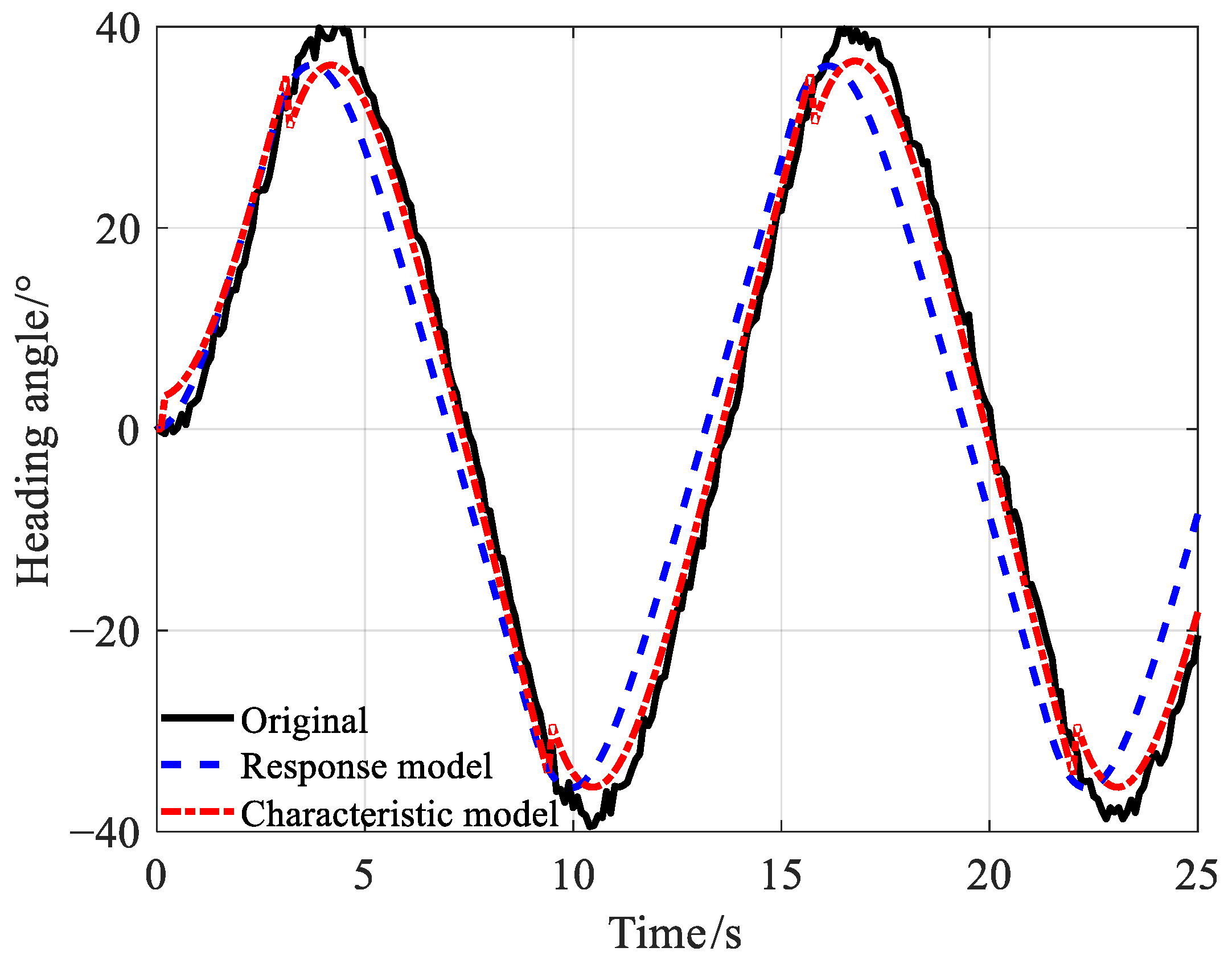
It is observed that from Figure 4, the characteristic model can better meet the identification demands. However, a leap occurs in the characteristic model’s identification result, which is mainly caused by the large data sampling interval. By the numerical analysis, it can be weakened in a short data sampling interval. Thus, the characteristic model can be used in the system identification of marine crafts.
Further, the RMSE and MAE are introduced to assess the accuracy, and the corresponding comparative results are shown in Table 1, which reveals that the characteristic model outperforms the response model in terms of accuracy. This indicates that the characteristic model can effectively capture the dynamics and characteristics of marine crafts and can provide more accurate and reliable identification results.

5.2. Comparison and Analysis of the Conventional LS-SVM Method and the CH-LS-SVM Method

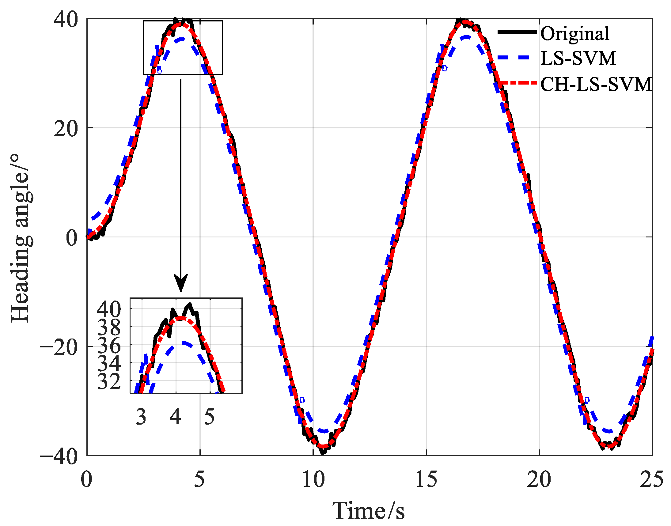
In order to densify and smooth the dataset, a data preprocessing strategy based on the CH interpolation algorithm is proposed. The results identified by the conventional LS-SVM method and the CH-LS-SVM method are shown in Figure 5.
As shown in Figure 5, the leap at the characteristic model’s identification result is weakened by the CH-based data preprocessing strategy, and the identification performance is further improved. It can be seen that the CH-based data preprocessing strategy is efficient for solving the problem of low identification accuracy due to long sampling intervals. Subsequently, the RMSEs and MAEs comparisons are listed in Table 2. Moreover, the deficiency of sensors-induced sampling limitation can be improved in the experiments. The results in Table 2 demonstrate the significant improvement in identification accuracy achieved with the CH-based approach in comparison to traditional methods. Overall, the CH-based data preprocessing strategy is a promising approach for enhancing the accuracy and efficiency of model identification and can be applied to a wide range of ocean engineering applications.

5.3. Validation of CH-WLS-SVM Method Improved by Multi-Kernel Function

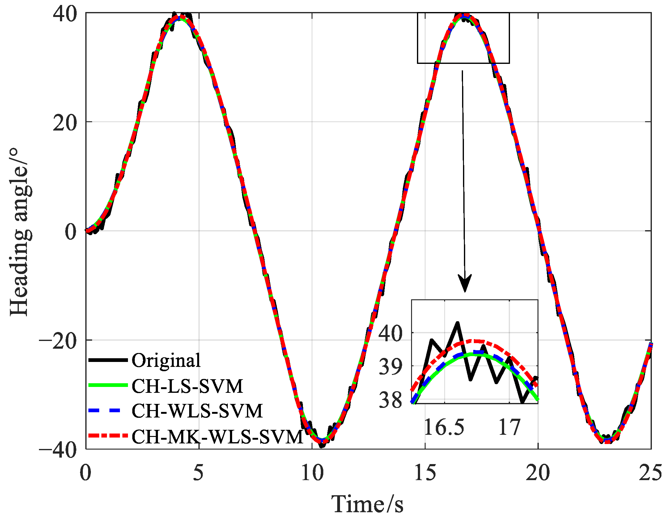
It is well known that the linear kernel function is a global kernel function, and the Gaussian kernel function is a local kernel function. Thus, the CH-MK-WLS-SVM method is designed to render the global and local performance improvements of the above WLS-SVM method. In the CH-MK-WLS-SVM method, the weighting control factor a in Equation (19) is chosen as 0.15 through numerical analysis, and the RMSE is 0.0938°. Specifically, the RMSE is 0.1432° and 0.1511° when a is 0 or 1, respectively. The identification results based on the characteristic model by using the CH-LS-SVM method, CH-WLS-SVM method, and CH-MK-WLS-SVM method are shown in Figure 6.
As can be seen from Figure 6, by adding the multi-kernel function into the CH-WLS-SVM method, the identification result of the CH-MK-WLS-SVM method is the most accurate, and it can fit well with the true values in the presence of sensor noise. And the performance improvements between these methods can be attributed to the validity of the proposed strategy that combines a novel weighting method with a multi-kernel function integration. Further, the RMSEs, MAEs, Root Mean Squared Log Error (RMSLE), and Adjusted R Squared (AR2) comparative results are listed in Table 3.
The tuning of the hyperparameters for the machine learning algorithms is very important and can seriously impact the performance of the algorithms. For the parameter selection of the study, the data are divided into the training and testing datasets. Besides, the hyperparameters are tuned within the set value through iterative optimization based on the RMSE of the testing dataset. For instance, in the tuning process for the LS-SVM, the hyperparameters (penalty factor C and RBF variable) are selected through iterative optimization, which aims to minimize the RMSE of the prediction results in the testing dataset. The C is tuned to 101–106, and the RBF variable is tuned to 0.1–5, which is shown in Figure 7.
Finally, the NN algorithm is selected as a comparative method to verify the superiority of the proposed strategy. In NN, the number of hidden Neurons is 10. The input variables are the heading angle and the rudder angle, in which the training data is 70% of the total, and others are used to test. The comparative result is shown in Figure 8. Through the numerical simulation of the 30° Zigzag test in MATLAB software, the RMSE is 0.0320. Compared to the CH-MK-MK-WLS-SVM (RMSE = 0.0087), the latter is superior in maneuvering prediction.

5.4. Experimental Study on a Marine Craft

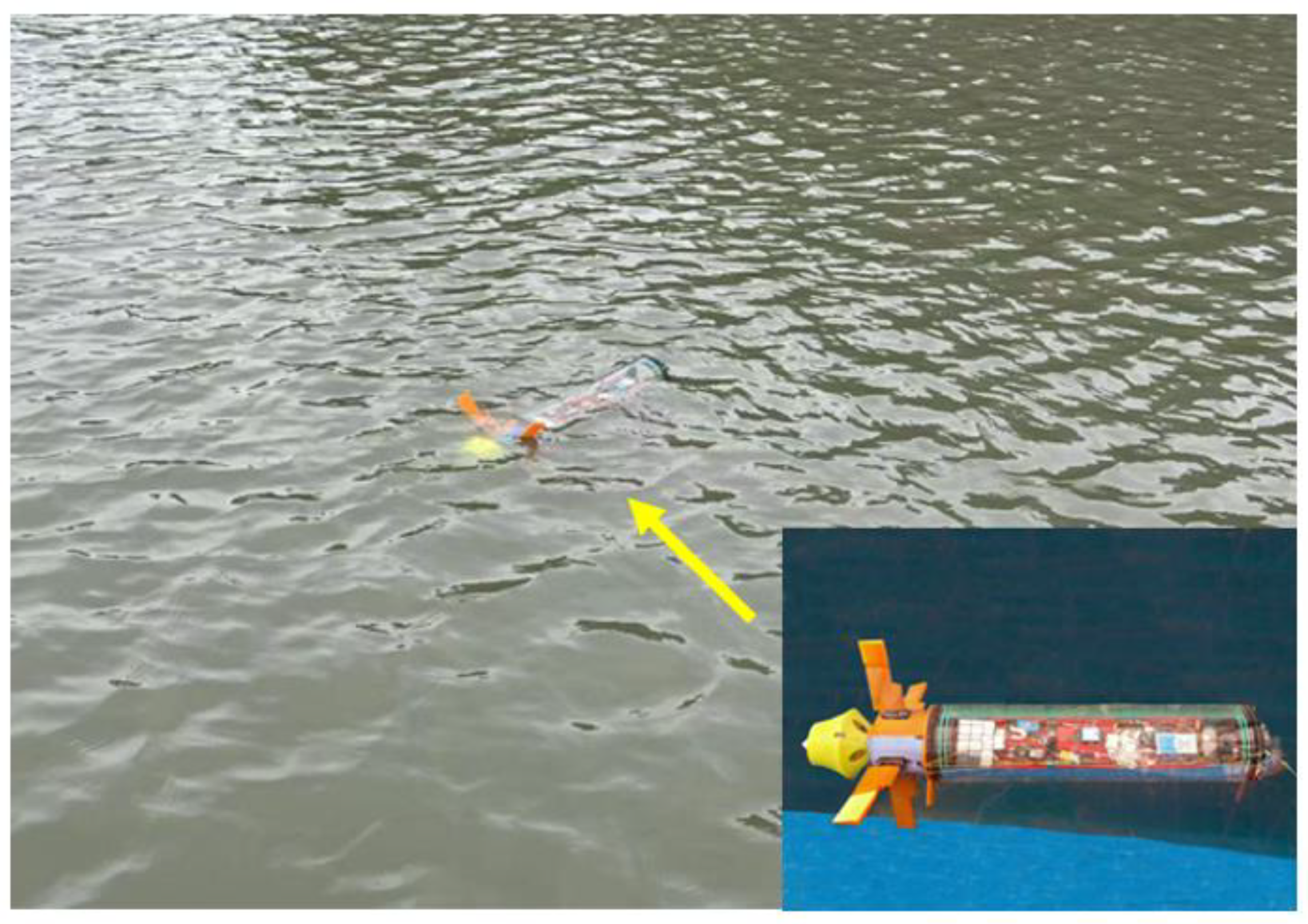
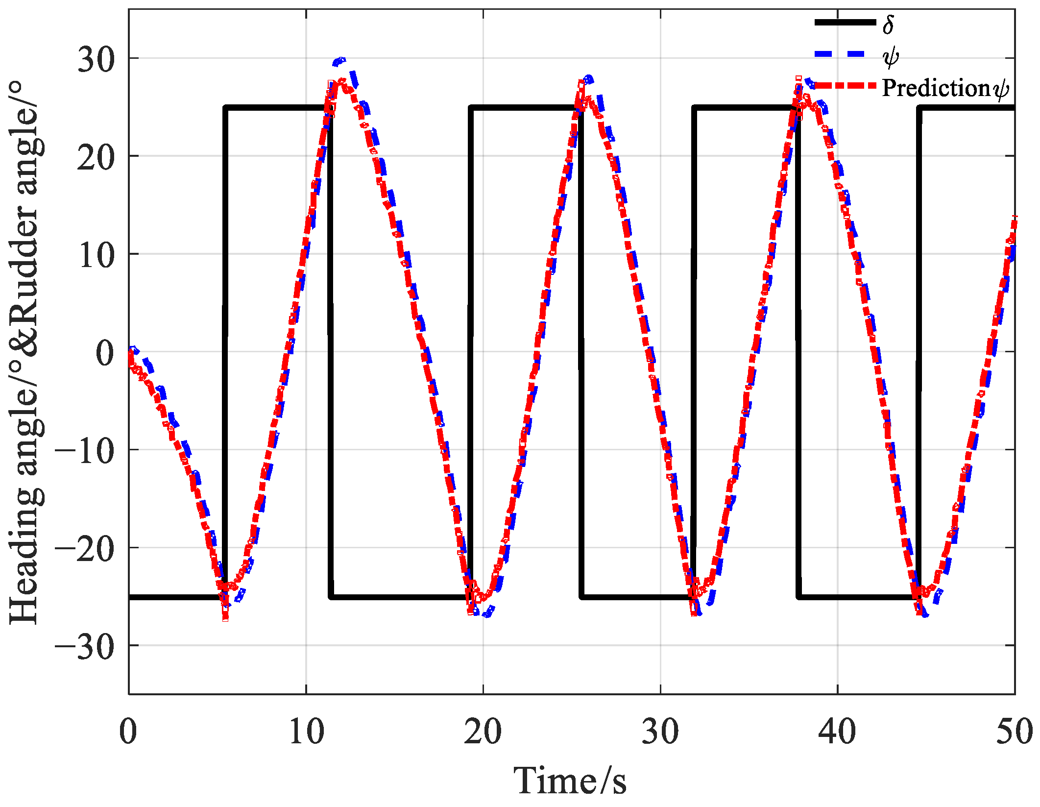
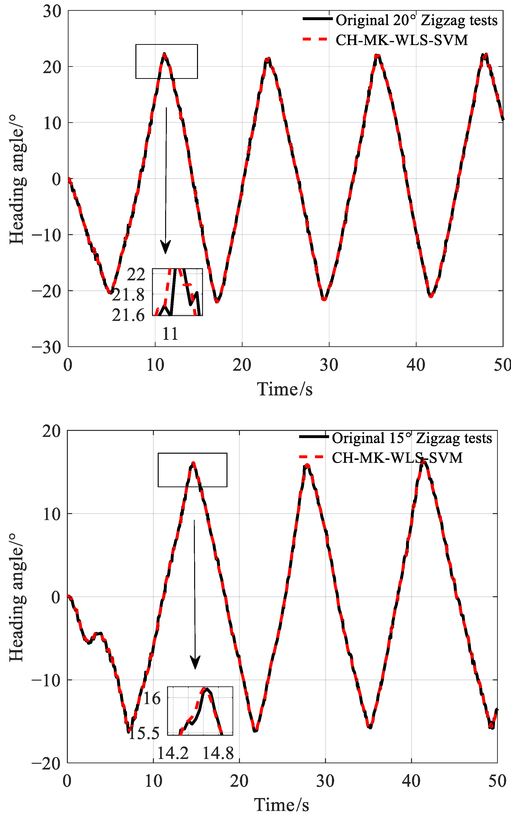
A marine craft shown in Figure 9 carried out a series of Zigzag maneuvering experiments in Zhi Yuan Lake at Shanghai Jiao Tong University under relatively calm water conditions. Table 4 illustrates the particulars of the marine craft for reference. Furthermore, modules such as a wireless transceiver unit, an attitude sensor (Angle resolution = 0.0055°), and an STM32F407 microcontroller are equipped on the marine craft. In this study, experimental studies are carried out under MATLAB 2018 environment and run at 2.3 GHz (CPU) and 24 GB memory (RAM). Then, a set of samples, including the actual rudder angle and heading angle, are collected. Finally, the 25° Zigzag maneuvering experiment is used as the training data; meanwhile, the 20° and 15° Zigzag maneuvering experiments provide the validation data to verify the predictive ability of the method. The training data and the identification result are shown in Figure 10.
To further evaluate the performance of the CH-MK-WLS-SVM method, additional experiments were conducted using different maneuvering angles. The prediction results of the 20° and 15° Zigzag maneuvering experiments based on the CH-MK-WLS-SVM method are shown in Figure 11, where the predictions are compared with the original data. The RMSE values obtained for the 20° and 15° maneuvers were 0.2497° and 0.1585°, respectively. These low RMSE values indicate that the CH-MK-WLS-SVM method is capable of providing highly accurate predictions of a marine craft’s heading angle during maneuvering operations.
Overall, the results of this study demonstrate that the CH-MK-WLS-SVM method is a promising approach for predicting a marine craft’s heading angle under various operating conditions. The proposed strategy is robust and accurate, making it a useful tool for marine engineers and operators concerned with vessel navigation and maneuvering. With further validation and refinement, this strategy could be widely deployed in the marine industry to improve safety, efficiency, and performance.

6. Conclusions

In this work, a hybrid system identification method based on the characteristic model named the CH-MK-WLS-SVM method is proposed for marine crafts, which provides an offline accurate identification method for marine crafts. The CH-MK-WLS-SVM method is verified by numerical simulation and experiments. The following advantages and features of the method can be summarized: Firstly, by introducing the CH-based interpolation algorithm, the data can be effectively densified and smoothed, which can improve the identification performance in the situation of missing data. Secondly, in order to further accurate identification, a novel weight method for the conventional WLS-SVM is designed. Thirdly, the linear kernel function and the Gaussian kernel function are combined to render global and local performance improvements of the method. Finally, the predictive capability of the CH-MK-WLS-SVM method is tested by using the data obtained from the 20° and 15° Zigzag maneuvering experiments. The results indicate that the CH-MK-WLS-SVM method is adequate to describe and predict the marine craft’s motion. Compared with the original identification result, the RMSE of the CH-MK-WLS-SVM method is reduced by an order of magnitude in the numerical simulation. Meanwhile, the good identification performance and predictive ability are verified through the experimental data.

7. Limitations and Future Studies

There are also some limitations of this study: (1) there are many parameters in the proposed multi-kernel WLS-SVM algorithm; hence, the selection of the parameters for the multi-kernel WLS-SVM algorithm is relatively time-consuming. (2) Although the proposed strategy has been verified by numerical simulation tests and experiments, experimental disturbances such as wind and wave disturbance are not considered. (3) The motion model only describes one direction in the horizontal plane, which is hard to predict other velocities in other DOFs.
In future studies, more work is needed to investigate techniques for choosing hyperparameters of the proposed method appropriately and conveniently, such as the penalty factor and the Gaussian kernel parameter. Moreover, verifying the proposed method in the multi-DoFs is also worthwhile to explore in the future.

Author Contributions

T.P.: Conceptualization, Methodology, Simulation, Writing—original draft; C.Y.: Conceptualization, Methodology, Writing—review & editing; Y.Z.: Methodology, Formal analysis; J.C.: Formal analysis, Supervision; L.L.: Supervision, Funding acquisition. All authors have read and agreed to the published version of the manuscript.

Funding

This research was supported in part by the National Natural Science Foundation of China under Grant 51909161, in part by the Natural Science Foundation of Shanghai under Grant 22ZR1434600, in part by the Oceanic Interdisciplinary Program of Shanghai Jiao Tong University under Grants SL2022MS016 and 2020QY10, and in part by the Shanghai Underwater Robot Engineering Technology Innovation Center under Grant 21DZ2221600.

Institutional Review Board Statement

Not applicable.

Informed Consent Statement

Not applicable.

Data Availability Statement

Not applicable.

Conflicts of Interest

The authors declare no conflict of interest.

References

  1. Shome, S.N.; Nandy, S.; Pal, D.; Das, S.K.; Vadali, S.R.K.; Basu, J.; Ghosh, S. Development of modular shallow water AUV: Issues & trial results. J. Inst. Eng. (India) Ser. C 2012, 93, 217–228. [Google Scholar]
  2. Morice, C.; Veres, S.; McPhail, S. Terrain referencing for autonomous navigation of underwater vehicles. In Proceedings of the Oceans 2009-Europe, Bremen, Germany, 11–14 May 2009; pp. 1–7. [Google Scholar]
  3. Allotta, B.; Costanzi, R.; Ridolfi, A.; Salvetti, O.; Reggiannini, M.; Kruusmaa, M.; Salumae, T.; Lane, D.M.; Frost, G.; Tsiogkas, N.; et al. The ARROWS project: Robotic technologies for underwater archaeology. IOP Conf. Ser. Mater. Sci. Eng. 2018, 364, 012088. [Google Scholar] [CrossRef]
  4. Kimura, R.; Choyekh, M.; Kato, N.; Senga, H.; Suzuki, H.; Ukita, M.; Kamezuka, K. Guidance and control of an autonomous underwater robot for tracking and monitoring spilled plumes of oil and gas from seabed. In Proceedings of the Twenty-third International Offshore and Polar Engineering Conference, Anchorage, AK, USA, 30 June–5 July 2013; pp. 366–371. [Google Scholar]
  5. Yu, C.; Xiang, X.; Lapierre, L.; Zhang, Q. Robust magnetic tracking of subsea cable by AUV in the presence of sensor noise and ocean currents. IEEE J. Ocean. Eng. 2018, 43, 311–322. [Google Scholar] [CrossRef]
  6. Włodarczyk-Sielicka, M.; Połap, D.; Prokop, K.; Połap, K.; Stateczny, A. Spatial visualization based on geodata fusion using an autonomous unmanned vessel. Remote Sens. 2023, 15, 1763. [Google Scholar] [CrossRef]
  7. Połap, D.; Wawrzyniak, N.; Włodarczyk-Sielicka, M. Side-scan sonar analysis using ROI analysis and deep neural networks. IEEE Trans. Geosci. Remote Sens. 2022, 60, 4206108. [Google Scholar] [CrossRef]
  8. Yu, C.; Zhong, Y.; Lian, L.; Xiang, X. Adaptive simplified surge-heading tracking control for underwater vehicles with thruster’s dead-zone compensation. Nonlinear Dyn. 2023. [Google Scholar] [CrossRef]
  9. Abkowitz, M.A. Measurement of hydrodynamic characteristics from ship maneuvering trials by system identification. SNAME Trans. 1980, 88, 283–318. [Google Scholar]
  10. Yoshimura, Y. Mathematical model for manoeuvring ship motion (MMG Model). In Proceedings of the Workshop on Mathematical Models for Operations involving Ship-Ship Interaction, Tokyo, Japan, 4–5 August 2005; pp. 1–6. [Google Scholar]
  11. Nomoto, K.; Taguchi, T.; Honda, K.; Hirano, S. On the steering qualities of ships. Int. Shipbuild. Prog. 1957, 4, 354–370. [Google Scholar] [CrossRef]
  12. Wu, H.; Wang, Y.; Xing, Y. Intelligent control based on intelligent characteristic model and its application. Sci. China Ser. F Inf. Sci. 2003, 46, 225. [Google Scholar] [CrossRef]
  13. Wen, Y.; Tao, W.; Zhu, M.; Zhou, J.; Xiao, C. Characteristic model-based path following controller design for the unmanned surface vessel. Appl. Ocean Res. 2020, 101, 102293. [Google Scholar] [CrossRef]
  14. Gokce, M.K.; Kinaci, O.K. Numerical simulations of free roll decay of DTMB 5415. Ocean Eng. 2018, 159, 539–551. [Google Scholar] [CrossRef]
  15. Perrault, D.; Bose, N.; O’Young, S.; Williams, C.D. Sensitivity of AUV response to variations in hydrodynamic parameters. Ocean Eng. 2003, 30, 779–811. [Google Scholar] [CrossRef]
  16. Hou, X.; Zou, Z.; Liu, C. Nonparametric identification of nonlinear ship roll motion by using the motion response in irregular waves. Appl. Ocean Res. 2018, 73, 88–99. [Google Scholar] [CrossRef]
  17. Holzhüter, T. Robust Identification scheme in an adaptive track-controller for ships. In Adaptive Systems in Control and Signal Processing; Elsevier: Amsterdam, The Netherlands, 1990; pp. 461–466. [Google Scholar]
  18. Zhong, Y.; Yu, C.; Wang, R.; Pei, T.; Lian, L. Adaptive anti-noise least-squares algorithm for parameter identification of unmanned marine vehicles: Theory, simulation, and experiment. Int. J. Fuzzy Syst. 2023, 25, 369–381. [Google Scholar] [CrossRef]
  19. Caccia, M.; Indiveri, G.; Veruggio, G. Modeling and identification of open-frame variable configuration unmanned underwater vehicles. IEEE J. Ocean. Eng. 2000, 25, 227–240. [Google Scholar] [CrossRef]
  20. Yin, J.; Zou, Z.; Xu, F. Parametric identification of Abkowitz model for ship maneuvering motion by using partial least squares regression. J. Offshore Mech. Arct. Eng. 2015, 137, 031301. [Google Scholar]
  21. Zhong, Y.; Yu, C.; Liu, C.; Liu, T.; Wang, R.; Lian, L. Recursive parameter identification for second-order K-T equations of marine robot in horizontal motion. Indian J. Geo-Mar. Sci. 2021, 50, 890–896. [Google Scholar]
  22. Sutulo, S.; Guedes Soares, C. An algorithm for offline identification of ship manoeuvring mathematical models from free-running tests. Ocean Eng. 2014, 79, 10–25. [Google Scholar] [CrossRef]
  23. Zhao, B.; Zhang, X.; Liang, C. A novel parameter identification algorithm for 3-DoF ship maneuvering modelling using nonlinear multi-innovation. J. Mar. Sci. Eng. 2022, 10, 581. [Google Scholar] [CrossRef]
  24. Golub, G.H.; Reinsch, C. Handbook series linear algebra singular value decomposition and least squares solutions. Numer. Math. 1970, 1970, 403–420. [Google Scholar] [CrossRef]
  25. Kalman, R.E. A new approach to linear filtering and prediction problems. J. Basic Eng. 1960, 82, 35–45. [Google Scholar] [CrossRef]
  26. Song, C.; Zhang, X.; Zhang, G. Nonlinear innovation-based maneuverability prediction for marine vehicles using an improved forgetting mechanism. J. Mar. Sci. Eng. 2022, 10, 1210. [Google Scholar] [CrossRef]
  27. Sabet, M.T.; Daniali, H.M.; Fathi, A.; Alizadeh, E. Identification of an autonomous underwater vehicle hydrodynamic model using the extended, cubature, and transformed unscented kalman filter. IEEE J. Ocean. Eng. 2018, 43, 457–467. [Google Scholar] [CrossRef]
  28. Dong, Z.; Yang, X.; Zheng, M.; Song, L.; Mao, Y. Parameter identification of unmanned marine vehicle manoeuvring model based on extended Kalman filter and support vector machine. Int. J. Adv. Robot. Syst. 2019, 16, 1–10. [Google Scholar] [CrossRef]
  29. Liu, Y.; Xue, Y.; Huang, S.; Xue, G.; Jing, Q. Dynamic model identification of ships and wave energy converters based on semi-conjugate linear regression and noisy input Gaussian process. J. Mar. Sci. Eng. 2021, 9, 194. [Google Scholar] [CrossRef]
  30. Vapnik, V. Universal learning technology: Support vector machines. NEC J. Adv. Technol. 2005, 2, 137–144. [Google Scholar]
  31. Luo, W.; Zou, Z.; Li, T. Application of support vector machine to ship steering. J. Shanghai Jiaotong Univ. (Sci.) 2009, 14, 462–466. [Google Scholar] [CrossRef]
  32. Luo, W.; Zou, Z. Parametric identification of ship maneuvering models by using support vector machines. J. Ship Res. 2009, 53, 19–30. [Google Scholar] [CrossRef]
  33. Pei, T.; Yu, C.; Zhong, Y.; Lian, L. Adaptive event-triggered mechanism-based online system identification framework for marine craft. Ocean Eng. 2023, 278, 114572. [Google Scholar] [CrossRef]
  34. Xu, H.; Hassani, V.; Guedes Soares, C. Truncated least square support vector machine for parameter estimation of a nonlinear manoeuvring model based on PMM tests. Appl. Ocean Res. 2020, 97, 102076. [Google Scholar] [CrossRef]
  35. Xu, H.; Hinostroza, M.A.; Wang, Z.; Guedes Soares, C. Experimental investigation of shallow water effect on vessel steering model using system identification method. Ocean Eng. 2020, 199, 106940. [Google Scholar] [CrossRef]
  36. Suykens, J.A.K.; De Brabanter, J.; Lukas, L.; Vandewalle, J. Weighted least squares support vector machines: Robustness and sparse approximation. Neurocomputing 2002, 48, 85–105. [Google Scholar] [CrossRef]
  37. Zhu, M.; Sun, W.; Hahn, A.; Wen, Y.; Xiao, C.; Tao, W. Adaptive modeling of maritime autonomous surface ships with uncertainty using a weighted LS-SVR robust to outliers. Ocean Eng. 2020, 200, 107053. [Google Scholar] [CrossRef]
  38. Xiang, G.; Xiang, X. 3D trajectory optimization of the slender body freely falling through water using cuckoo search algorithm. Ocean Eng. 2021, 235, 109354. [Google Scholar] [CrossRef]
  39. Zhang, S.; Zhang, X.; Hu, S. Characteristic model-based ship motion mathematical model. Navig. China 2012, 35, 63–65. [Google Scholar]
  40. Xia, Y.; Xu, K.; Huang, Z.; Wang, W.; Xu, G.; Li, Y. Adaptive energy-efficient tracking control of a X rudder AUV with actuator dynamics and rolling restriction. Appl. Ocean Res. 2022, 118, 102994. [Google Scholar] [CrossRef]
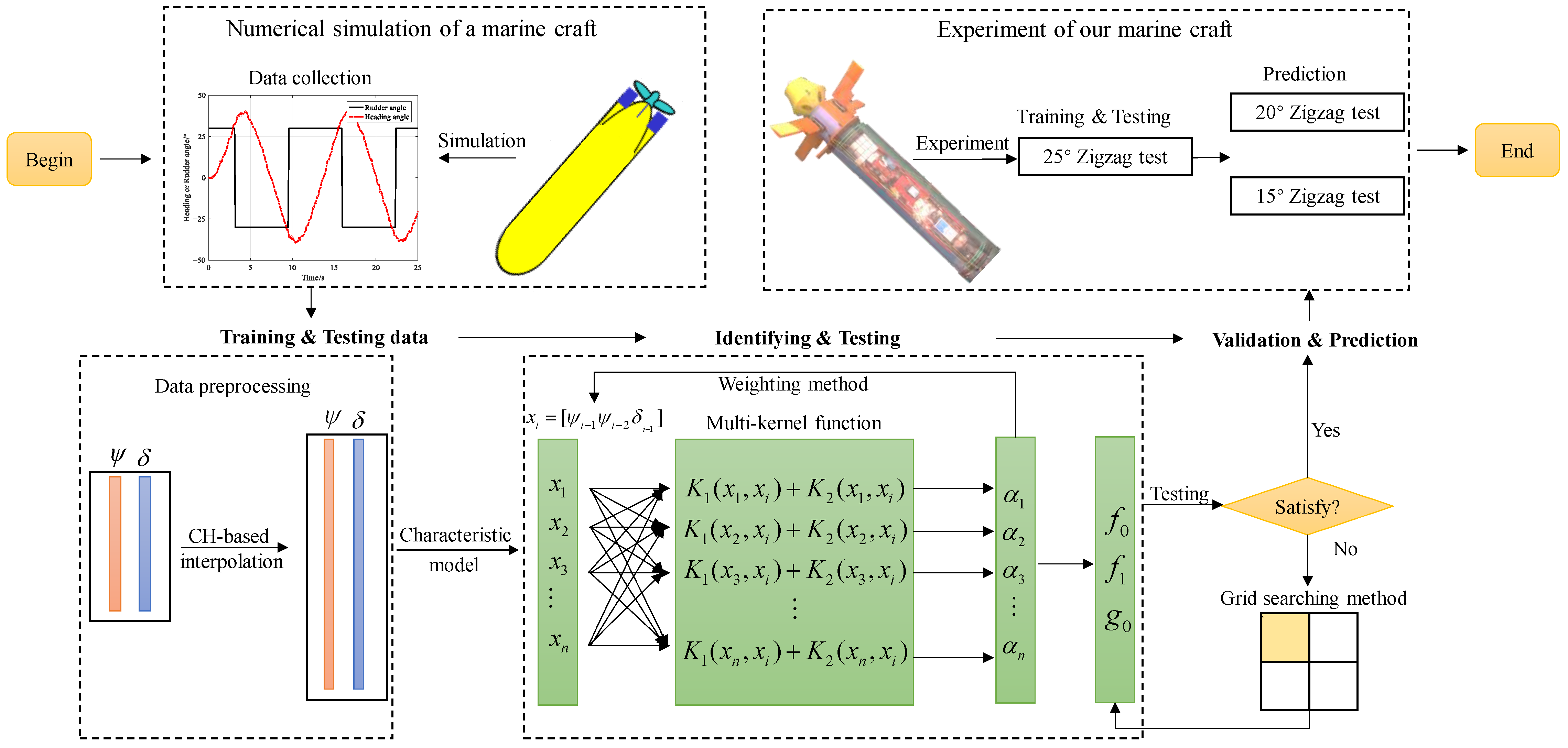
Figure 1. The flowchart of the identification process.
Jmse 11 01091 g001
Figure 2. The white noise in the data.
Jmse 11 01091 g002
Figure 3. The training data, including the heading and rudder angle (control input) from Zigzag tests.
Jmse 11 01091 g003
Figure 4. The comparison of the response model and the characteristic model.
Jmse 11 01091 g004
Figure 5. The comparison of the conventional LS-SVM method and the CH-LS-SVM method.
Jmse 11 01091 g005
Figure 6. The comparison of the CH-LS-SVM method, CH-WLS-SVM method, and CH-MK-WLS-SVM method.
Jmse 11 01091 g006
Figure 7. The tuning process of the hyperparameters.
Jmse 11 01091 g007
Figure 8. The tuning process of the hyperparameters.
Jmse 11 01091 g008
Figure 9. The marine craft.
Jmse 11 01091 g009
Figure 10. The identification result of the 25° Zigzag maneuvering experiment.
Jmse 11 01091 g010
Figure 11. Predictions of the 20° and 15° Zigzag maneuvering experiments.
Jmse 11 01091 g011
Table 1. The RMSEs and MAEs of the response model and the characteristic model.
Response ModelCharacteristic Model
RMSE (°)7.00562.6748
MAE (°)6.13862.6453
Table 2. The RMSEs and MAEs of the conventional LS-SVM method and the CH-LS-SVM method.
LS-SVMCH-LS-SVM
Sampling interval (s)0.50.17
RMSE (°)2.67980.2301
MAE (°)2.64530.1864
Table 3. The RMSEs and MAEs of the above methods.
CH-LS-SVM
(Linear Kernel Function)
CH-WLS-SVM
(Linear Kernel Function)
CH-WLS-SVM
(Gaussian Kernel Function)
CH-MK-WLS-SVM
(Multi-Kernel Function)
RMSE (°)0.20080.15110.14320.0938
MAE (°)0.18430.13060.12030.0781
RMSLE (°)0.35390.27070.21040.1655
AR20.99940.99950.99950.9996
Table 4. Main technical characteristics of the marine craft.
DescriptionValue
Length (m)0.85
Mass (kg)7.8
Rudder’s area (cm2)40
Attitude sensor’s resolution (°)0.0055
Servo’s maximum torque (kg·cm)40
Disclaimer/Publisher’s Note: The statements, opinions and data contained in all publications are solely those of the individual author(s) and contributor(s) and not of MDPI and/or the editor(s). MDPI and/or the editor(s) disclaim responsibility for any injury to people or property resulting from any ideas, methods, instructions or products referred to in the content.