Abstract
An effective path-following controller is a guarantee for stable sailing of underactuated unmanned surface vehicles (USVs). This paper proposes an event-triggered robust control approach considering an unknown model nonlinearity, external disturbance, and event-triggered mechanism. The proposed method consists of guidance and dynamic control subsystems. Based on the tracking error dynamics equations, the guidance subsystem is designed to achieve the guidance law. For the dynamic control subsystem, the radial basis function neural networks (RBFNNs) are designed to approximate the unknown model nonlinearity and external disturbances to improve the robustness of the proposed method. In addition, an event-triggered mechanism is constructed to reduce the triggering times. The closed-loop system is proven to be stable, and the effectiveness of the proposed method is illustrated through simulation results.
1. Introduction
An unmanned surface vehicle (USV) is a kind of autonomous waterborne platform that can autonomously complete tasks, such as environmental perception and target detection, and has autonomous identification, autonomous planning, and autonomous navigation capabilities [1,2,3]. It has the advantages of small size, low cost, good maneuverability, and no casualties [4]. The USV can independently perform tasks in areas where manned ships are not suitable for dispatch, thereby expanding the scope of water operations. Therefore, it has become an important tool in carrying out civilian and military tasks such as marine environmental monitoring, water search and rescue, ship escort, firepower strike, and anti-submarine tasks [5].
In complex marine environments, ensuring the safety, stability, and accuracy of autonomous navigation for USVs is a major challenge for USV control systems. The overall issues of motion control for USVs include set-point regulation, trajectory tracking, and path following [6].
In the motion control system of USVs, the existing propulsion system usually consists of the main thruster and rudder or the double thrusters at the stern of the ship, without side thrusters. This power configuration means that the USVs have only two control inputs. However, there are three degrees of freedom (DoF) for USVs, including surge, sway, and yaw, which means that the number of control inputs is less than the DoF of the USVs. This type of USV has underactuated characteristics. Because of the low maneuverability, it is more suitable to study the path following control of underactuated USVs.
Path following refers to USVs tracking a predetermined path. The USV does not need to reach a certain position on the path at the specified time, and the reference path is independent of time. In other words, the spatial constraints of path following problem take precedence over time constraints. As shown in Figure 1, the path following control of USVs divides the control system into two parts: the guidance subsystem and the control subsystem. Based on the path information and environmental information, the guidance subsystem generates the expected reference signals. Then, the control subsystem will track the reference signal generated by the guidance subsystem to achieve path tracking. Path tracking control is similar to the actual behavior of crew maneuvering ships, and the modular design concept allows it to directly apply mature guidance technology and heading maintenance control theory, which has strong practical application value and has become a commonly used solution for USV path following.
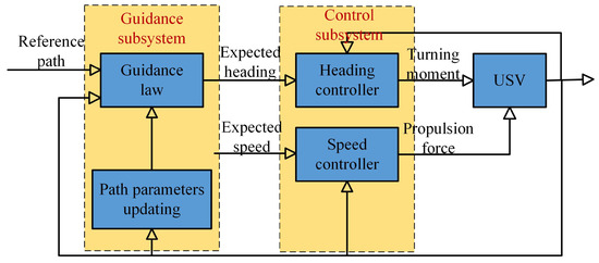
Figure 1.
Schematic diagram of path following control framework.
Over the last several years, promising results on the path following control of USVs have been proposed.
From the perspective of guidance subsystem, the commonly used guidance algorithms are line-of-sight (LOS)-based methods [7,8,9,10,11].
In [7], a LOS-based guidance law was designed for target enclosing control of an USV, and the effectiveness of the proposed method was verified by simulations and experiments. However, when the tracking error is large, the speed of LOS method converging to the desired path is relatively slow. In addition, when the USV is influenced by the environment disturbance, the sideslip angle will occur, which limits the application of the LOS method. In order to deal with the above-mentioned problem, Fossen et al. proposed an integral LOS in [8] using additional integral terms to offset the sideslip angle. Moreover, there are many improvement methods based on LOS. In [9], an adaptive LOS guidance law was proposed for the finite-time path following control of USVs, which can keep the tracking error within the constraint range. In [10], the fuzzy rules were used to determine the forward looking distance of the LOS guidance to increase the convergence speed. In [11], based on sliding mode theory, a robust LOS guidance law was designed for the underactuated ships. Except for LOS-based approaches, the vector field guidance is also widely used in USV control [12,13,14].
From the perspective of control subsystem, there are many approaches applied to the USV control field and that have achieved good control results. The approaches include proportional integration differentiation (PID) [15,16,17], trajectory linearization control (TLC) [18,19,20], sliding mode control (SMC) [21,22,23], backstepping [9,24,25,26], and intelligent control [27,28,29,30,31].
As a most widely used algorithm applied to USV path following control, PID controller has the advantages of simple structure, good economy, and high control accuracy. However, when external disturbances exist, such as wind, waves, and currents, the adaptability of the PID controller is insufficient and its control stability will decrease. Currently, researches on PID control method have mainly focused on its improvements. For instance, in [15] the authors proposed an improved PID control method by using optimization theory, and this method can obtain the optimal control parameters. In [16], the fuzzy rules were used to realize the self adjustment of PID parameters to improve its robustness. In [17], a modified incremental PID was proposed to deal with the influence of the marine currents. Trajectory linearization can simplify the problem of path following control. However, linearization processing will lead to system errors and reduce control accuracy. Similar to other algorithms, we can combine it with robust control approaches improve control performance. In [18], to improve the robust performance of the TLC approaches, the neural network (NN) is used to estimate the model uncertainties. In [19], the linear extended state observer was designed to approximate the unknown disturbances, and by combining with the TLC approach, a robust controller was proposed for USVs. In [20], a finite-time disturbance observer was designed to observe disturbance and uncertainties to improve the robustness of TLC method. SMC has robustness to parameter changes and external disturbances; however, it has the disadvantage of chattering. In [21], by using hyperbolic tangent function, a SMC-based path following controller was proposed for the USV, which can deal with the chattering problem. In [22], the SMC was used to structure an observer. Then, it was combined with the adaptive law, and a nonlinear surge controller was proposed. In [23], to achieve fast converge speed, a nonsingular terminal SMC was designed for the USV control in the present of model uncertainties. The backstepping method is greatly influenced by the motion model, and in order to achieve good control performance and robustness, it is necessary to establish an accurate model—which is difficult to obtain. Therefore, for the backstepping approach, combinations with other techniques (for instance, tracking error compensation [9], SMC [26]) to improve its robustness performance have been a research hotspot. Intelligence control methods have unique advantages in dealing with nonlinear and complex system problems. Fuzzy logic control converts expert knowledge into fuzzy rules, which can effectively deal with the impact of model uncertainty and interference in the path following control of USVs [27]. In addition, NN can be used to approximate the uncertainty and external interference terms of the USV model, so as to improve the anti-interference ability and robustness of the controller [28,29]. In recent years, machine learning theory has developed rapidly, and reinforcement learning has been widely applied in the field of USV control [30,31]. Reinforcement learning theory does not require the establishment of accurate mathematical models, and has a self-learning ability in unknown environments. Therefore, it has great research value for solving model uncertainty and unknown interference problems in USV control.
Although fruitful research results have been reported, we need to note that limitations and challenges still exist:
- The control methods in most existing works on path following control of USVs are time triggered (e.g., [15,26]), which means that the control signals should update at every sampling instance, and it is unnecessary from the perspective of resource allocation;
- The USV model is highly nonlinear and coupled, which poses great difficulties in the design of path following controllers. Currently, although there are many papers studying the nonlinear controller design of USVs, most methods still require knowledge of partial or complete model information (e.g., [9,25]).
Inspired by the existing literature discussed above, this paper proposes a event-triggered robust path following controller subject to unknown model nonlinearity and disturbances. Specifically, based on the relative position between the USV and the expected path, a dynamic equation for its path tracking error is established in the Serret–Frenet coordinate system. According to the backstepping technique and Lyapunov stability theory, the guidance law and control signals are achieved. Then, to deal with the unknown model nonlinearity and disturbances, radial basis function neural networks (RBFNNs) are designed. Finally, on the basis of the above mentioned control signals, an event-triggered mechanism is structured to obtain the final control inputs. The contributions of this paper are summarized as follows:
- An event-triggered based path following controller is proposed for the underactuated USVs. Because of the event-triggered mechanism, there is no need to update the control inputs at every sample instance. Therefore, this can decrease the computational burden;
- The RBFNNs are designed to approximate the model nonlinearity and disturbances, which makes the proposed controller not rely on the USV mathematical model and improves the robustness performance of the controller.
The organization of the rest is as follows. In Section 2, several useful lemmata are provided. In Section 3, the USV model and the control objectives are given. The guidance subsystem is presented in Section 4, and the design process of an event-triggered robust controller is proposed in Section 5. Then, the closed-loop system is proved to be stable in Appendix A. The effectiveness is verified in Section 6 by simulations. Finally, the conclusion and potential future studies are given in Section 7.
2. Preliminary
For the following nonlinear system,
where x is the system state, and the equilibrium point is .
Lemma 1.
Define as the Lyapunov function about state x of system (1), and it is radially bounded. If the following two conditions are satisfied: (1) ; (2) ; (3) is uniformly continuous, then, we can say that the system is globally asymptotically stable.
Lemma 2.
If the Lyapunov function about state x of system (1) meets with , where , then, we can say that the system is globally uniformly ultimately bounded (GUUB).
Lemma 3.
The nonlinear term of system (1) can be approximated by the RBFNN with arbitrary accuracy:
where ω is the weight vector of the RBFNN, is the vector consists of Gaussian function , and the approximation error δ and weight ω are all bounded.
3. Problem Formulation
In this section, the mathematical model of the USV and the control objectives are given.
3.1. USV Model
The kinematics model of the USV is
where is its position, is the yaw angle, u is its surge velocity, v is its sway velocity, and r is its yaw angular velocity.
The dynamics model of the underactuated USV is [4,6]
where and are the model parameters of the USV, is the force in the surge channel, is the yaw torque in the yaw channel, and , , and are the disturbances in each DoF.
3.2. Control Objectives
The purpose of this paper is to propose a path following control approach for underactuated USV considering unknown model nonlinearity, disturbances, and an event-triggered mechanism. The following conditions should be satisfied:
- The underactuated USV can converge to a desired path P, which means , where and are the position tracking errors defined in the following content;
- The underactuated USV can sail along the desired path at a predefined surge velocity , which means ;
- The controller can guarantee the USV moves stably under the influence of unknown model nonlinearity and disturbances;
- A suitable event-triggered mechanism should be designed.
4. Guidance Subsystem Design for Path Following Control of Underactuated USV
In this section, the tracking error dynamic equations are given, and the guidance law is derived.
As shown in Figure 2, is the position vector of the USV in the inertial coordinate system , and the velocity vector can be . The course angle can be calculated by
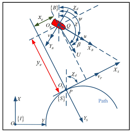
Figure 2.
Path following diagram of the underactuated USV.
From Figure 2, we have
where is the sideslip angle of the USV.
Therefore, the kinematics model of the USV can be re-expressed in a Serret–Frenet coordinate system as
where .
It is assumed that P is a point moving along the path at a designed velocity , where is the path parameter to be designed.
Then, the course error is
where is the course angle of point P.
The displacement vector between Q and P is ; therefore, the relative velocity can be calculated by . The angular velocity of P can be expressed as , where is the path curvature and is the parameter to be designed.
In the frame, we have
where is the rotation matrix, , , and
Then, we can obtain
The derivation of Equation (8) is
Therefore, the tracking error dynamic equations can be
To achieve objective 1 in Section 3.2, we define the following Lyapunov function as
where and .
Then, is presented as
The speed can be designed as
where .
Then, can be rewritten as
where and . We choose here, then .
Finally, the desired yaw angular velocity can be designed as
where , and .
Based on Lemma 1, the system is globally asymptotically stable.
To sum up, if the yaw angular velocity of the USV r changes according to Equation (17), and the path parameter and the velocity of guidance point P change according Equation (15), then the tracking errors , and will converge to zero, which means that objective 1 in Section 3.2 will be achieved.
5. Control Subsystem Design for Path Following Control of Underactuated USV
In this section, the dynamic controller is designed.
5.1. Backstepping-Based Dynamic Controller Design
Define the tracking error of the surge velocity as
where is the desired surge velocity.
To achieve objective 2 in Section 3.2, we define the following Lyapunov function as
Differentiating Equation (20), we can obtain
where , which contains the nonlinear term and the disturbance.
The control signal in the surge channel can be
where .
For yaw channel, to track the desired yaw angular velocity , we define the following Lyapunov function
where .
Differentiating Equation (23), we can obtain
where , and .
In the same way, the control signal in yaw channel can be
where .
Therefore, if the control inputs are given by the following equations, the underactuated USV can track the desired path P.
The objectives 1 and 2 in Section 3.2 can be achieved under control input given by Equation (26).
However, it should be noted that the control signals contains nonlinearities and disturbances where it is very difficult to obtain their accurate expressions. Therefore, to achieve objective 3 in Section 3.2, the RBFNNs are designed to approximate the nonlinear terms and disturbances in Equation (26).
Remark 1.
By using a backstepping approach, we can decompose the USV system into two subsystems, with one handling the position variable and the other handling the velocity variable. Virtual control laws are designed for each subsystem to achieve stability, and Lyapunov stability analysis is performed to ensure the overall system stability. Specifically, in Section 4, the position tracking of the USV is achieved by designing the desired velocity variables and . The control laws and are then designed in Section 5 to ensure the USV can navigate with the desired velocities.
5.2. Radial Basis Function Neural Networks Design
To estimate the term , we define the following RBFNN:
where is the ideal weight vector of the NN, is the vector consists of Gaussian functions, is the NN input, and is the error.
Because the ideal weights are very difficult to obtain, then we define the estimated value of as
where is the estimated value of , and is short for .
Then the control input Equation (22) can be
Define the following Lyapunov function as
where is the estimation error of the weights vector and is a positive defined matrix.
Differentiating Equation (30), we can obtain
Then, the updating law of can be
where .
In the same way, to estimate the term , we define the following RBFNN:
where is the ideal weight vector of the NN, is the vector consists of Gaussian functions, is the NN input, and is the error.
Because the ideal weights are very difficult to obtain, then we define the estimated value of as
where is the estimated value of , and is short for .
Then the control input Equation (25) can be
Define the following Lyapunov function as
where is the estimation error of the weights vector and is a positive defined matrix.
Differentiating Equation (36), we can obtain
Then, the updating law of can be
where .
Therefore, considering the unknown nonlinearity and disturbances, the control inputs below can guarantee the USV to track along the desired path P, which means that the control objectives 1 to 3 in Section 3.2 can be achieved under the control input given by Equation (39).
However, the controller is time triggered, which means the control input should update at every sampling instance. To deal with this problem, an event-triggered mechanism is designed in the following subsection.
5.3. Event-Triggered Mechanism Design
The event-triggered mechanism in surge channel can be designed as
where , , and is the ith triggered instance. is the virtual signal to be designed. During the period from to , the control signal will hold constant as . The next event will be triggered when , and the control signal will become .
Based on Equation (40), for , we have . Therefore, the following equation is obvious
where is a time-varying parameter satisfying , and .
Recalling Equation (30), we have
Then, the virtual control signal can be designed as
where and .
In the same way, for the yaw channel, the event-triggered mechanism can be designed as
where , , and is the jth triggered instance. is the virtual signal to be designed. During the period from to , the control signal will hold constant as . The next event will be triggered when , and the control signal will become .
Based on Equation (45), for , we have . Therefore, the following equation is obvious
where is a time-varying parameter satisfying , , and .
Recalling Equation (36), we have
Then, the virtual control signal can be designed as
where and .
Therefore, the proposed event-triggered RBFNN-based controller for the surge channel is as follows
The controller for the yaw channel is as follows
At this point, all the control objectives 1 to 4 in Section 3.2 are achieved.
Based on the above content, we can draw the following theorem.
Theorem 1.
The proof of Theorem 1 can be found in Appendix A.
6. Simulation Results
To verify the effectiveness of the proposed controller, simulations are carried out. The model parameters are listed in Table 1, which can also be found in [4,6].

Table 1.
Parameters of the USV.
Two cases are included in this section. In case 1, the control performances with different controller parameters are evaluated, which helps us choose appropriate controller parameters. In case 2, comparisons with other methods are made to reflect the superiority of the proposed method.
The simulation platform used in this paper is MATLAB and the equation solver is a fourth–fifth-order Runge–Kutta algorithm (ODE45).
6.1. Case 1: Performance with Different Controller Parameters
In this case, the desired path is given by
where .
The initial position of the USV is m m, its initial yaw angle rad, its initial surge velocity m/s, its initial lateral velocity m/s, its initial yaw angular velocity is rad/s, the simulation time is 120 s, the simulation step s, and no external disturbances are considered in this case.
The states m/s], m/s, 0.5 m/s], and rad/s, 0.2 rad/s] are selected as the input of the RBFNNs; the node number of each NN is 21; the Gaussian function width of the RBFNN in the surge channel is , the width of the RBFNN in the yaw channel is , and the center is uniformly distributed; and the initial weights are all .
The simulation results are shown in Figure 3, Figure 4, Figure 5 and Figure 6 (take , , neuron number, and for example). Please note that in these figures, R is set as 40 m.
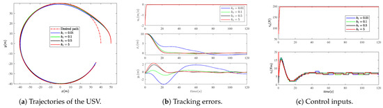
Figure 3.
Tracking results with different values ().
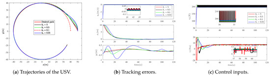
Figure 4.
Tracking results with different values ().
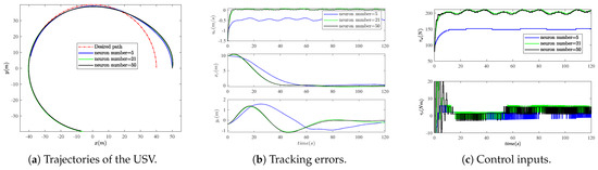
Figure 5.
Tracking results with different neuron numbers ().
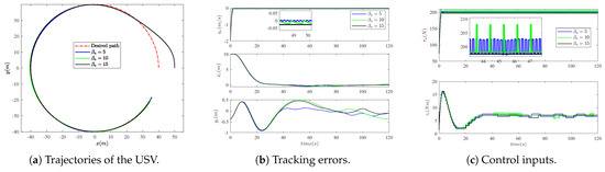
Figure 6.
Tracking results with different values ().
As shown in Figure 3a, we can see that even though the value of is different, the USV can still track the desired path with high accuracy. However, the smaller the value of , the slower the USV converges to the desired path, as illustrated in Figure 3b. It can be found that the event-triggered mechanism plays a role in the path-following of the USV, where the control inputs are only updated when the event is triggered as shown in Figure 3c. By comparison, the value of is ultimately chosen as .
From Figure 4a, it can be seen that the USV is still able to accurately tack the desired path even when different values of are selected. Different from , the value of not only affects the convergence speed to the desired path, but also affects the tracking accuracy of the surge velocity, which is illustrated in Figure 4b. The smaller the value of is, the smaller the surge velocity tracking error will be. However, the smaller the value of is, the slower the USV converges to the desired path. In addition, It can be found that the value of will also affect the number of event triggers. The larger the value of , the more times the event will be triggered as shown in Figure 4c. By comparison, the value of is ultimately chosen as .
The node number of the RBFNN is determined by comparing the control performance with different node numbers. As shown in Figure 5, we can find that when the number of neurons is five, although the USV can move along the desired path, it exhibits a significant forward velocity tracking error. However, when the number of neurons is 21 or 50, their control performances are similar. Since a larger number of neurons requires more computational time, the final number of neurons is chosen to be 21.
A illustrated in Figure 6a, it can be observed that the value of has little impact on the accuracy of path tracking for the USV. The value of primarily affects the event-triggered times in surge channel, which in turn affects the tracking precision of surge velocity. It is clear that the smaller the , the more times the event will be triggered. By comparison, the value of is ultimately chosen as 15.
Finally, all the controller parameters are listed in Table 2.
Table 2.
Controller parameters.
The simulation is carried out to verify the vehicle behavior for a smaller m. In this condition, four different initial states are selected: m, 0, rad], = [0, 15 m, rad], m, rad], and = [0, −15 m, 0]. The controller parameters are listed in Table 2. The results are shown in Figure 7.
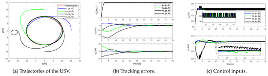
Figure 7.
Tracking results with different initial states ().
6.2. Case 2: Comparison with Other Approaches
In this case, other two approaches including backstepping and time triggered RBFNN-based backstepping are involved. The control laws of these two controllers are given by Equations (26) and (39).
The initial states of the USV, the desired path, the set of the RBFNNs are all the same as case 1. The desired surge velocity in this case is m/s, and the external disturbance is .
The simulation results are shown in Figure 8 and Figure 9, and the control performance comparisons are listed in Table 3.
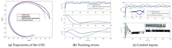
Figure 8.
Tracking results with different control methods ().
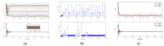
Figure 9.
Weights of the RBFNNs, triggering time intervals, and the estimated values of the RBFNNs. (a) Weights of the RBFNNs. (b) Triggering instants and time intervals in each channel. (c) Estimated value of the RBFNN in each channel.
Table 3.
Performance comparison.
Integral absolute error (IAE) can be calculated by , where and T is the simulation duration. Root mean square error (RMSE) can be calculated by .
Integrating the errors in IAE captures the cumulative effect of position tacking errors over the entire interval, providing a quantitative measure of the overall error. RMSE evaluates the root mean square of the errors, which measures the dispersion between the desired position and the true position of the USV, providing an overall understanding of the error distribution. Therefore, the selection of IAE and RMSE as evaluation metrics is aimed at comprehensively considering the cumulative effect and distribution characteristics of position tracking errors. They provide a thorough assessment of the differences between the desired position and the actual position of the USV and help compare the performance of the algorithms.
From Figure 8a,b, it can be observed that the control accuracy of the backstepping method tends to decrease significantly due to the external disturbances. However, for RBFNN-backstepping and the proposed method, due to the robustness of the NN, the USV can still track the desired path with high accuracy. As shown in Figure 8c, the control inputs only update when the event is triggered.
As shown in Figure 9a, each weight of the RBFNN in the surge and yaw channels is bounded. The triggering time intervals in each channel are illustrated in Figure 9b. It can be found that the maximum time intervals can reach up to s and s. Considering the unknown model nonlinearity and external disturbances, . Submitting the model parameters listed in Table 1, we can obtain . After the system stabilizes, the lateral velocity and yaw angular velocity of the USV are relatively small. Hence, the actual value of will also be small (taking the example at s, the actual value of is only ). Therefore, the weights of the RBFNN in the yaw channel are very small as shown in Figure 9c.
From Table 3, we can find that, for the backstepping method, the IAE and RMSE of position are much bigger than the ones of RBFNN-based backstepping approach or the proposed method (backstepping: , proposed method: , and RBFNN-based backstepping: ). The fundamental reason for this situation is that the traditional backstepping technique is a model-based method and its robustness is poor, while the RBFNN can improve the robustness of the other two approaches. Comparing the proposed method with RBFNN-based backstepping, the difference between the IAE and RSME of the proposed method and the ones of the RBFNN-based backstepping are very small. However, the triggering times of the proposed method in both the surge and yaw channels are much less than the ones of the RBFNN-based backstepping method (proposed method: 77 times in the surge channel and 293 times in the yaw channel; RBFNN-based backstepping: 12,000 times in both channels).
Above all, it is clear that the proposed method can guarantee the USV to track the desired path accurately even if the unknown model nonlinearity and disturbances exist. In addition, profiting from the designed event-triggered mechanism, which is different from the time-triggered control approaches, there is no need for the proposed method to update the control inputs at every sampling instant.
Although the control method proposed in this paper ensures stable navigation of the USV under the influence of unknown nonlinearity and external disturbances, there is still room for further improvement. For example, the method does not consider control input constraints, the neural network structure parameters are manually set without optimization, and it does not take into account the consideration of optimal performance criteria.
Remark 2.
In Appendix A, the closed-loop system is proven to be GUUB, and we obtain the following inequality:
By solving the above inequality, we can obtain the following results:
where denotes the initial value of .
Therefore, the tracking error satisfies:
where
Based on the above analysis, it can be concluded that the tracking error is bounded as time progresses. Therefore, it is possible that there are some errors that do not converge to zero.
7. Conclusions
In this paper, we proposed an event-triggered robust controller for underactuated USVs to enhance their path-following capabilities. The guidance law is derived based on the dynamic equations of the tracking error. To enhance the robustness of our approach, we employed RBFNNs to approximate unknown nonlinearities and external disturbances. Furthermore, we introduced event-triggered mechanisms that update control inputs only when specific events occur. The simulation results demonstrated the effectiveness of the proposed event-triggered robust controller and exhibited a strong robustness and a significant reduction in triggering times.
In future research, we aim to address additional challenges, such as actuator saturation, state constraints, and energy optimization. These aspects will be incorporated to further enhance the performance and applicability of the proposed controller.
Author Contributions
Conceptualization, W.Z.; methodology, W.Z.; software, W.Z.; validation, M.N., J.R. and J.X.; formal analysis, W.Z.; investigation, M.N.; resources, M.N.; data curation, J.R.; writing—original draft preparation, W.Z.; writing—review and editing, W.Z.; visualization, W.Z.; supervision, W.Z.; project administration, W.Z.; funding acquisition, W.Z. All authors have read and agreed to the published version of the manuscript.
Funding
This work was supported by National Natural Science Foundation of China (No. 62203293). It was also sponsored by the Shanghai Rising-Star Program (No. 22YF1416100).
Institutional Review Board Statement
Not applicable.
Informed Consent Statement
Not applicable.
Data Availability Statement
No new data were created or analyzed in this study. Data sharing is not applicable to this article.
Conflicts of Interest
The authors declare no conflict of interest.
Appendix A. Stability Analysis
Proof of Theorem 1.
Consider the following Lyapunov function:
By differentiating Equation (A1), we can obtain
Because
Equation (A4) can be re-expressed as
If , we can obtain
If , we can obtain
It should be noted that no matter what value takes, the value of . In the same way, .
Therefore, we have the following equation:
Note that
Therefore,
Based on Young’s inequality, it is clear that
Therefore,
Because
then we can obtain
where , and .
From Lemma 2, , , , and are all bounded; therefore, is bounded. Based on the above content, the closed-loop system is GUUB according to Lemma 3.
Remark A1.
Based on Lemma 2, to guarantee that the closed-loop system is GUUB, the Lyapunov function should meet with , where and are all positive constants. In this paper, is the minimum value among and . To ensure that is always a positive constant, the values of and should be positive. Therefore, both and should be greater than .
In addition, the event-triggered based controller should avoid the Zeno behavior.
For the surge channel, by recalling , we have
It is clear that , and are bounded; therefore, a positive constant exists, such that .
Because and , the time interval , which means the Zeno behavior is avoided.
In the same way, it is easy to prove that the Zeno behavior in the yaw channel can also be avoided.
At this point, the proof of Theorem 1 is completed. □
References
- Zhang, L.; Ji, X.; Jiao, Y.; Huang, Y.; Qian, H. Design and Control of the “TransBoat”: A Transformable Unmanned Surface Vehicle for Overwater Construction. IEEE/ASME Trans. Mechatron. 2023, 28, 1116–1126. [Google Scholar] [CrossRef]
- Cheng, P.; Zhang, C.; Xie, W.; Zhang, W.; He, S. Network-Based Adaptive Multievent-Triggered Fuzzy Dynamic Positioning Controller Design for Unmanned Surface Vehicles Against Denial-of-Service Attacks. IEEE Trans. Control Netw. Syst. 2023, 10, 612–624. [Google Scholar] [CrossRef]
- Peng, Z.; Jiang, Y.; Liu, L.; Shi, Y. Path-Guided Model-Free Flocking Control of Unmanned Surface Vehicles Based on Concurrent Learning Extended State Observers. IEEE Trans. Syst. Man Cybern. Syst. 2023, 53, 4729–4739. [Google Scholar] [CrossRef]
- Zhou, W.; Wang, Y.; Ahn, C.K.; Cheng, J.; Chen, C. Adaptive Fuzzy Backstepping-Based Formation Control of Unmanned Surface Vehicles with Unknown Model Nonlinearity and Actuator Saturation. IEEE Trans. Veh. Technol. 2020, 69, 14749–14764. [Google Scholar] [CrossRef]
- Ren, Y.; Zhang, L.; Ying, Y.; Li, S.; Tang, Y. Model-Parameter-Free Prescribed Time Trajectory Tracking Control for Under-Actuated Unmanned Surface Vehicles with Saturation Constraints and External Disturbances. J. Mar. Sci. Eng. 2023, 11, 1717. [Google Scholar] [CrossRef]
- Zhou, W.; Fu, J.; Yan, H.; Du, X.; Wang, Y.; Zhou, H. Event-Triggered Approximate Optimal Path-Following Control for Unmanned Surface Vehicles With State Constraints. IEEE Trans. Neural Networks Learn. Syst. 2023, 34, 104–118. [Google Scholar] [CrossRef] [PubMed]
- Jiang, Y.; Peng, Z.; Wang, D.; Chen, C.L.P. Line-of-Sight Target Enclosing of an Underactuated Autonomous Surface Vehicle With Experiment Results. IEEE Trans. Ind. Inform. 2020, 16, 832–841. [Google Scholar] [CrossRef]
- Fossen, T.I.; Pettersen, K.Y.; Galeazzi, R. Line-of-Sight Path Following for Dubins Paths With Adaptive Sideslip Compensation of Drift Forces. IEEE Trans. Control Syst. Technol. 2015, 23, 820–827. [Google Scholar] [CrossRef]
- Tong, H. An adaptive error constraint line-of-sight guidance and finite-time backstepping control for unmanned surface vehicles. Ocean Eng. 2023, 285, 115298. [Google Scholar] [CrossRef]
- Xiu, Y.; Li, D.; Deng, H.; Jiang, S.; Wu, E.Q. Path-Following Based on Fuzzy Line-of-Sight Guidance for a Bionic Snake Robot With Unknowns. IEEE-ASME Trans. Mechatron. 2023; Early Access. [Google Scholar] [CrossRef]
- Liu, C.; Guo, W.; Sun, T. RLOS-based path following with event-triggered roll motion control for underactuated ship using rudder. Ocean Eng. 2023, 269, 113592. [Google Scholar] [CrossRef]
- Wen, Y.; Tao, W.; Zhu, M.; Zhou, J.; Xiao, C. Characteristic model-based path following controller design for the unmanned surface vessel. Appl. Ocean Res. 2020, 101, 102293. [Google Scholar] [CrossRef]
- Gong, X.; Liu, L.; Peng, Z. Safe-critical formation reconfiguration of multiple unmanned surface vehicles subject to static and dynamic obstacles based on guiding vector fields and fixed-time control barrier functions. Ocean Eng. 2022, 250, 110821. [Google Scholar] [CrossRef]
- Wang, M.; Su, Y.; Wu, N.; Fan, Y.; Qi, J.; Wang, Y.; Feng, Z. Vector field-based integral LOS path following and target tracking for underactuated unmanned surface vehicle. Ocean Eng. 2023, 285, 115462. [Google Scholar] [CrossRef]
- Song, L.; Xu, C.; Hao, L.; Yao, J.; Guo, R. Research on PID Parameter Tuning and Optimization Based on SAC-Auto for USV Path Following. J. Mar. Sci. Eng. 2022, 10, 1847. [Google Scholar] [CrossRef]
- Yuan, J.; Zhang, W.; Liu, H.; Li, H. Heading and speed joint control of double-push USV based on fuzzy PID. Int. J. Robot. Autom. 2023, 38, 32–41. [Google Scholar] [CrossRef]
- Yu, P.; Zhou, Y.; Sun, X.; Sang, H.; Zhang, S. Adaptive path following control for wave gliders in ocean currents and waves. Ocean Eng. 2023, 284, 115251. [Google Scholar] [CrossRef]
- Qiu, B.; Wang, G.; Fan, Y.; Mu, D.; Sun, X. Robust path-following control based on trajectory linearization control for unmanned surface vehicle with uncertainty of model and actuator saturation. IEEJ Trans. Electr. Electron. Eng. 2019, 14, 1681–1690. [Google Scholar] [CrossRef]
- Qiu, B.; Wang, G.; Fan, Y.; Mu, D.; Sun, X. Adaptive LOS Path Following based on Trajectory Linearization Control for Unmanned Surface Vehicle with Multiple Disturbances and Input Saturation. Control Eng. Appl. Inform. 2019, 21, 76–87. [Google Scholar]
- Qiu, B.; Wang, G.; Fan, Y.; Mu, D.; Sun, X. Path Following of Underactuated Unmanned Surface Vehicle Based on Trajectory Linearization Control with Input Saturation and External Disturbances. Int. J. Control Autom. Syst. 2020, 18, 2108–2119. [Google Scholar] [CrossRef]
- Yan, Y.; Yu, S.; Gao, X.; Wu, D.; Li, T. Continuous and Periodic Event-Triggered Sliding-Mode Control for Path Following of Underactuated Surface Vehicles. IEEE Trans. Cybern. 2023. [Google Scholar] [CrossRef]
- Yan, Z.; Feng, W.; Wang, H. Adaptive surge control of variable-mass unmanned surface vehicle based on sliding mode observation. Ocean Eng. 2023, 269, 113576. [Google Scholar] [CrossRef]
- Wu, G.X.; Ding, Y.; Tahsin, T.; Atilla, I. Adaptive neural network and extended state observer-based non-singular terminal sliding modetracking control for an underactuated USV with unknown uncertainties. Appl. Ocean Res. 2023, 135, 103560. [Google Scholar] [CrossRef]
- Feng, Z.; Pan, Z.; Chen, W.; Liu, Y.; Leng, J. USV Application Scenario Expansion Based on Motion Control, Path Following and Velocity Planning. Machines 2022, 10, 310. [Google Scholar] [CrossRef]
- Li, Y.; Zhang, J.; Wang, H.; Li, Y.; Sui, B. Research on Heading Control of USV with the Lateral Thruster. Math. Probl. Eng. 2022, 2022, 8359227. [Google Scholar] [CrossRef]
- Zhao, Y.; Sun, X.; Wang, G.; Fan, Y. Adaptive Backstepping Sliding Mode Tracking Control for Underactuated Unmanned Surface Vehicle With Disturbances and Input Saturation. IEEE Access 2021, 9, 1304–1312. [Google Scholar] [CrossRef]
- Taghieh, A.; Zhang, C.; Alattas, K.A.; Bouteraa, Y.; Rathinasamy, S.; Mohammadzadeh, A. A predictive type-3 fuzzy control for underactuated surface vehicles. Ocean Eng. 2022, 266, 113014. [Google Scholar] [CrossRef]
- Wang, R.; Li, D.; Miao, K. Optimized Radial Basis Function Neural Network Based Intelligent Control Algorithm of Unmanned Surface Vehicles. J. Mar. Sci. Eng. 2020, 8, 210. [Google Scholar] [CrossRef]
- Liao, Y.; Chen, C.; Du, T.; Sun, J.; Xin, Y.; Zhai, Z.; Wang, B.; Li, Y.; Pang, S. Research on disturbance rejection motion control method of USV for UUV recovery. J. Field Robot. 2023, 40, 574–594. [Google Scholar] [CrossRef]
- Woo, J.; Yu, C.; Kim, N. Deep reinforcement learning-based controller for path following of an unmanned surface vehicle. Ocean Eng. 2019, 183, 155–166. [Google Scholar] [CrossRef]
- Wang, Y.; Cao, J.; Sun, J.; Zou, X.; Sun, C. Path Following Control for Unmanned Surface Vehicles: A Reinforcement Learning-Based Method With Experimental Validation. IEEE Trans. Neural Netw. Learn. Syst. 2023; Early Access. [Google Scholar] [CrossRef]
Disclaimer/Publisher’s Note: The statements, opinions and data contained in all publications are solely those of the individual author(s) and contributor(s) and not of MDPI and/or the editor(s). MDPI and/or the editor(s) disclaim responsibility for any injury to people or property resulting from any ideas, methods, instructions or products referred to in the content. |
© 2023 by the authors. Licensee MDPI, Basel, Switzerland. This article is an open access article distributed under the terms and conditions of the Creative Commons Attribution (CC BY) license (https://creativecommons.org/licenses/by/4.0/).