Analytical Solution of Time-Optimal Trajectory for Heaving Dynamics of Hybrid Underwater Gliders

Abstract

Underwater vehicles have capacity limits for control inputs, within which their time-optimal trajectories (TOTs) can be formulated. In this study, the fastest trajectory for the depth control of a hybrid underwater glider (HUG) was found using buoyancy engines and propellers individually, and the decoupled heave dynamics of the HUG were defined using quadratic hydrodynamic damping. Because buoyancy engines always run at slow speeds, the buoyancy force was formulated based on the constant force rate of the engine. It was assumed that the nominal value of the heave dynamics parameters could be estimated; therefore, the analytical solution of heave dynamics could be formulated using the thrusting saturation and constant buoyancy force rate. Then, the shortest trajectory for depth control of the HUG could be established while considering the actuator saturation. To verify the effectiveness of the TOT in HUG heave dynamics, extensive tracking control simulations following the TOT were conducted. It was found that the proposed TOT helps the HUG reach the desired depth in the shortest arrival time, and its robust depth control showed good tracking performance in the presence of external bounded disturbances.

1. Introduction

With the advancement of oceanography research and marine resource exploration, underwater mobile platforms have gained prominence, assuming a pivotal role in various underwater missions including resource exploration, ocean observation, environmental monitoring, and sea area investigations [1,2,3]. These platforms come in various types, such as remotely operated vehicles (ROVs) [4,5,6], autonomous underwater vehicles (AUVs) [7,8,9], and underwater gliders (UGs) [10,11,12]. Among these, the underwater glider (UG) stands out as a buoyancy-driven autonomous robot capable of converting vertical motion into horizontal movement using airfoil technology, allowing it to move forward with minimal power consumption over extended periods [13]. Utilizing fixed wings, internal masses, a ballast pump, and a rudder, this glider controls its attitude and depth by adjusting buoyancy levels, gliding effortlessly through the water column. Due to its exceptional performance, traditional cylindrical UGs have garnered significant research attention [14,15].

UGs like the Slocum [16,17], Spray [18], Seaglider [19,20], and Deepglider [21,22] were originally developed for oceanographic applications. While these buoyancy-driven gliders have demonstrated impressive endurance and energy efficiency, they suffer from limitations in speed and maneuverability due to their restricted propulsion capabilities and external control surfaces. Hence, enhancing the efficiency of gliders necessitates a reconfiguration of their design [23,24,25]. One innovative approach to address these limitations involves the hybrid-driven UG equipped with a propeller, independently adjustable wings, and a controllable rudder. This innovative design incorporates a dual-mode propulsion system, augmenting the glider’s speed significantly. Moreover, the integration of controllable wings and a rudder enhances the glider’s maneuverability, thereby enhancing its overall versatility.

Trajectories play a pivotal role in governing the motion of autonomous systems, and their meticulous design is necessary for attaining high performance. Each underwater vehicle has a capacity limit for control inputs, including the maximum thrust of the propeller or the maximum net buoyancy force of the buoyancy engine. Time-optimal trajectories (TOTs) for these vehicles can be formulated within these constraints. Previous studies have focused on the TOT problem, such as the singular extremals of underwater vehicle systems in [26] and the design of time-efficient trajectories with constant thrust arcs in [27]. However, the latter algorithm required significant computational time for practical implementation. Rhoads et al. [28] presented a numerical method for minimum time heading control of an UG in known and time-varying flow fields. Meanwhile, Vu et al. [29] developed an energy-efficient trajectory for depth motion control in underwater vehicle systems. Their approach addressed uncertainties in bounded parameters and disturbances, utilizing a global optimal sliding mode controller with limited control input. Duc et al. [30] derived an analytical solution for the second-order nonlinear differential equation governing the heading motion of underwater vehicles. However, this research exclusively formulated the analytical solution for heading motion using propeller thrust saturation.

Achieving precise trajectory tracking amidst disturbances and uncertainties poses a significant challenge, particularly for nonlinear systems and notably in robotic systems [31,32,33]. Numerous control strategies have been proposed to address this issue, including sliding mode control [34,35], adaptive control [36,37], neural network control [38], backstepping control [39,40], dynamic surface control [41,42], etc. Among these approaches, sliding mode control (SMC) offers an effective approach to attain robust control for underactuated underwater vehicles. Its inherent discontinuity, characterized by switching characteristics, renders SMC a fitting choice for governing underactuated systems. Furthermore, SMCs exhibit well in handling-system parameter uncertainties and disturbances [43,44]; thus, SMC demonstrates remarkable robustness when applied to systems with uncertainties. The depth controller is imperative for an underwater vehicle to execute its mission successfully under the influence of environmental loads. Consequently, validating the performance of the designed controller through simulations becomes an indispensable step before any real-world trials. The HUG’s ability to track the desired depth is hindered by two major barriers, namely steady-state error and non-zero pitch angle. Inaccurate trim and ballasting conditions were found to be the cause of this issue in a previous study by Claus et al. [45], where the depth control of a HUG using a buoyancy engine and internal moving mass was described. However, this method resulted in considerable overshoot and steady-state error in depth-keeping control, with suboptimal settling time. To overcome these issues, this study aims to design an efficient trajectory for depth control of a HUG using a buoyancy engine and thruster, with the objective of eliminating overshoot and steady-state error while maintaining the desired depth.

In this study, the goal is to design a TOT for depth control in the HUG system using buoyancy-driven propulsion and a thruster individually. A closed-form solution is presented for the pure heave dynamics under each constraint of buoyancy and thrusting force. The control input is designed based on the limits of buoyancy force, buoyancy force rate, and thruster force, and the TOT for depth control is defined to satisfy the constraints of heave dynamics and actuator saturation. To track the TOT under the presence of external bounded disturbance, an SMC algorithm is designed, and its performance along with the proposed TOT will be verified through computer simulations.

The rest of this paper is organized as follows. The concept of TOTs for depth control of a HUG is presented in Section 2, followed by the closed-form solution of pure heave dynamics in Section 3, where maximum buoyancy force, maximum rate of buoyancy force, and minimum propeller force are considered. Section 4 defines the time-optimal trajectory, and Section 5 presents the design of robust tracking control using SMC. The robust tracking control with the proposed TOT will be simulated in Section 6 while considering the bounded disturbance. Finally, the conclusion presents the effectiveness of the proposed TOT and highlights the merits of the closed-form solution.

2. Heave Dynamics of Hybrid Underwater Glider and TOT Definition

2.1. Assumptions

In this paper, the motion of the HUG is simplified to focus solely on its heave motion. Some simplifications have been applied to enable feasible simulations of the HUG. These simplifications are outlined as follows:

• The HUG is assumed to have neutral buoyancy, with its body-fixed coordinate system centered at its mass center;
• The HUG is deeply submerged in a homogeneous, unbounded fluid, far removed from the free surface and devoid of surface effects;
• The HUG exhibits three planes of symmetry;
• To simplify the problem, only the depth motion of the HUG is considered in this paper;
• The hydrodynamic coefficients of the HUG remain constant and do not vary.

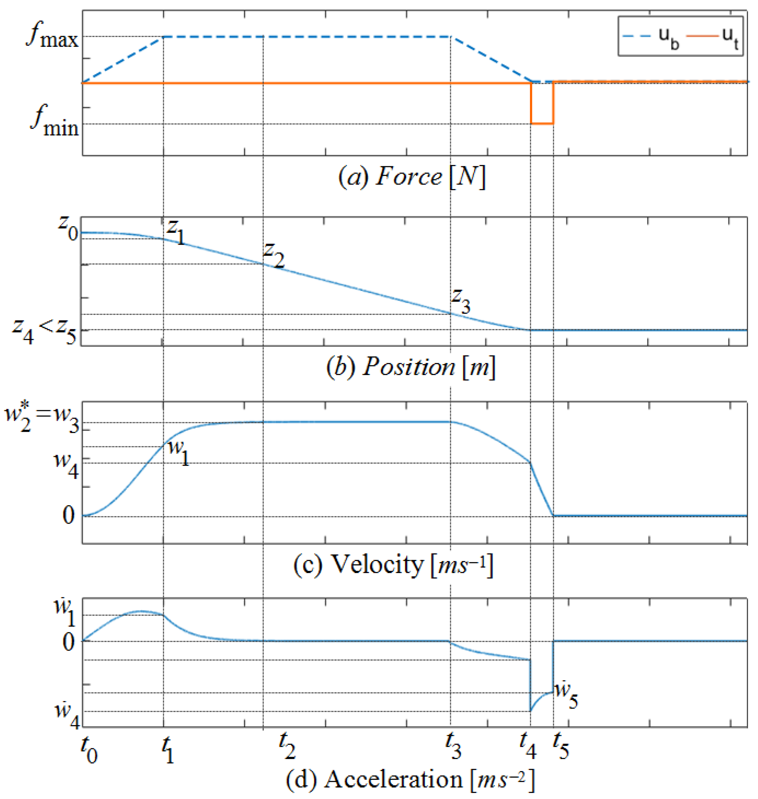
2.2. Heave Motion of HUG and TOT Definition

In this section, we propose a TOT for the heave control of HUGs, which is a challenging task due to the slow speed of the buoyancy engine. The TOT is based on the limitations of the buoyancy engine speed and saturation, as well as the thruster saturation. The six degrees-of-freedom (DOF) nonlinear equations of motion for an underwater vehicle are detailed in Fossen [46,47]. However, this paper specifically concentrates on depth control. Thus, we present the nonlinear second-order differential equation that characterizes the pure depth-plane motion of the HUG as follows:

$$\begin{array}{l}(m-Z_{\dot{w}})\dot{w}-Z_{w\left|w\right|}w\left|w\right|=(W-B)+Z_{prop}\\ \dot{z}=w\end{array}$$

(1)

where m, Z_ẇ, w, Z_w|w|, W, B, and Z_prop are the mass of the HUG, added mass coefficient, instantaneous velocity, cross-flow drag coefficient, weight of the HUG, buoyancy force, and thrust force, respectively.

The heave dynamics of HUGs, described by two first-order differential systems, can be represented by Equation (2), where $a=m-Z_{\dot{w}}$, $b=-Z_{\left|w\right|w}$, and f represent the control force acting on the vehicle, d is the external disturbance, $Z_{\dot{w}}$ is the added mass, and $Z_{\left|w\right|w}$ is the damping coefficient.

$$\begin{array}{l}a\dot{w}+b\left|w\right|w=f+d\\ \dot{z}=w\end{array}$$

(2)

This paper employs an analytical approach, distinct from numerical methods, to derive TOTs. These TOTs are represented as explicit functions within unchanged closed-form expressions, enhancing the controller’s autonomous capabilities. The proposed trajectory-tracking controller ensures optimal time performance when its references (inputs) align with the TOTs, even in the presence of uncertainties. The concept of a TOT is grounded in formulating the solution of the given dynamics as a time-dependent function for a specific control input. In this context, maintaining the control input at both maximum and minimum values during acceleration and deceleration times yields the closed-form time function representing the fastest or TOT for the given dynamics.

Table 1. Some variables used in the TOT.

Variables	Description
$f_{max}$	The maximum force applied to HUG
$f_{min}$	The minimum force applied to HUG
$z_0$	Initial depth of HUG
$z_5$	Desired depth of HUG
$w_{d1}$	The velocity profile of HUG in the 1st segment
$w_{d2}$	The velocity profile of HUG in the 2nd segment
$w_{d3}$	The velocity profile of HUG in the 3rd segment
$w_{d4}$	The velocity profile of HUG in the 4th segment
$w_{d5}$	The velocity profile of HUG in the 5th segment
$z_{d1}$	The position profile of HUG in the 1st segment
$z_{d2}$	The position profile of HUG in the 2nd segment
$z_{d3}$	The position profile of HUG in the 3rd segment
$z_{d4}$	The position profile of HUG in the 4th segment
$z_{d5}$	The position profile of HUG in the 5th segment
${\dot{w}}_{d1}$	The acceleration profile of HUG in the 1st segment
${\dot{w}}_{d2}$	The acceleration profile of HUG in the 2nd segment
${\dot{w}}_{d3}$	The acceleration profile of HUG in the 3rd segment
${\dot{w}}_{d4}$	The acceleration profile of HUG in the 4th segment
${\dot{w}}_{d5}$	The acceleration profile of HUG in the 5th segment

provides a definition of the terms used in the proposed TOT.

The HUG system utilizes two types of control forces: the net buoyancy force $u_b$ produced by the buoyancy engine and the thruster force $u_t$ generated by the thruster depicted in Figure 1. The buoyancy engine is employed for descent, requiring low energy consumption, while the thruster force is used sparingly when the vehicle approaches the desired depth and to maintain the HUG at that depth. By switching between these two forces, the HUG can be precisely controlled to reach the desired depth. To minimize the use of thruster force, it should only be applied once the vehicle attains neutral buoyancy.

The control strategy for the heaving motion of the HUG system is depicted in Figure 2a, which shows the buoyancy force of the buoyancy engine as a dashed blue line. The up slope and down slope represent the compression and expansion rates of air in the cylinder, respectively. The designed thruster force is represented by the solid orange line.

In order to control the depth of the HUG system, the constant rate of the buoyancy force needs to be considered. This constant rate of the buoyancy force can be expressed as $c_{max}$ and $c_{min}$ for the maximum and minimum speeds, respectively. Thus, the buoyancy force can be formulated as $c_{max}\left(t-t_0\right)$ and $c_{min}\left(t-\alpha \right)$, where $t_0$ and α are the initial times for the descending motion and neutral condition, respectively. To ensure precise depth control, it is necessary to define five different time periods, as described in Figure 2. The first segment is from $t_0$ to $t_1$, and the dynamics of this period can be deduced from Equation (3). It is important to note that $t_1=t_0+\frac{f_{max}}{c_{max}}$ plays a key role in this period. The dynamics equations for the second and third segments, which are from $t_1$ to $t_2$ and from $t_2$ to $t_3$, respectively, can be defined as Equation (4). Similarly, the dynamics of the fourth and fifth segments can be established as Equations (5) and (6), respectively. By solving all these dynamics, the TOT for the pure depth plant of the HUG system can be defined. However, it should be noted that this concept is only applicable during deep operation, as the HUG should reach maximum heaving velocity as depicted in Figure 2d, which can be expressed by the condition $z_5\ge \left(z_2-z_0\right)+\left(z_4-z_3\right)$. This concept is effective in achieving precise depth control at depths of several hundred meters.

$$a{\dot{w}}_d+b{w}_d^2=c_{max}\left(t-t_0\right)$$

(3)

$$a{\dot{w}}_d+b{w}_d^2=f_{max}$$

(4)

$$a{\dot{w}}_d+b{w}_d^2=c_{min}\left(t-\alpha \right)$$

(5)

$$a{\dot{w}}_d+b{w}_d^2=f_{min}$$

(6)

3. Analytical Solution of TOT in Heave Dynamics of HUG Using Buoyancy and Thruster Force Individually

3.1. TOT in the 1st Segment with Positive Force Rate from Buoyancy Engine

The heave dynamics in this segment can be described by Equation (7), which can be rewritten as Equation (8) by defining the variable $w_{d1}$ as $\frac{a}{b}\frac{\dot{y}}{y}$. The solution to Equation (8) involves the use of the Airy function, which can be solved using an alternative function y, as presented in Equation (9).

$$a{\dot{w}}_{d1}+b{w}_{d1}^2=c_{max}\left(t-t_0\right)$$

(7)

$$\begin{gathered} \frac{a^2}{b}\left(\frac{\ddot{y}}{y}-\frac{{\dot{y}}^2}{y^2}\right)+\frac{a^2{\dot{y}}^2}{b{y}^2}=c_{max}\left(t-t_0\right) \\ \iff \frac{a^2}{b}\frac{\ddot{y}}{y}=c_{max}\left(t-t_0\right) \end{gathered}$$

(8)

$$y\left(t\right)=a_0{y}_0\left(t\right)+a_1{y}_1\left(t\right)$$

(9)

To define the components of function $y\left(t\right)$, we can use the following equations:

$$y_0\left(t\right)=1+\frac{{\sigma }_1{\left(t-t_0\right)}^3}{6}+\frac{{\sigma }_1^2{\left(t-t_0\right)}^6}{180}+\frac{{\sigma }_1^3{\left(t-t_0\right)}^9}{12960}$$

(10)

$$y_1\left(t\right)=\left(t-t_0\right)+\frac{{\sigma }_1{\left(t-t_0\right)}^4}{12}+\frac{{\sigma }_1^2{\left(t-t_0\right)}^7}{504}+\frac{{\sigma }_1^3{\left(t-t_0\right)}^{10}}{45360}$$

(11)

$${\sigma }_1=\frac{b{c}_{max}}{a^2}$$

(12)

Having the function $y\left(t\right)$ defined, its first and second derivatives can be calculated as follows:

$$\dot{y}\left(t\right)=a_0{\dot{y}}_0\left(t\right)+a_1{\dot{y}}_1\left(t\right)$$

(13)

$$\ddot{y}\left(t\right)=a_0{\ddot{y}}_0\left(t\right)+a_1{\ddot{y}}_1\left(t\right)$$

(14)

Subsequently, the velocity trajectory can be represented as Equation (15) using the alternative function $y$, while the acceleration trajectory can be obtained by taking the derivative of the velocity trajectory, as presented in Equation (16). Finally, the position trajectory can be derived by integrating the velocity trajectory and is given by Equation (17), with $C_0$ defined as Equation (18).

$$w_{d1}=\frac{a}{b}\frac{\dot{y}}{y}$$

(15)

$${\dot{w}}_{d1}=\frac{a}{b}\left(\frac{\ddot{y}}{y}-\frac{{\dot{y}}^2}{y^2}\right)$$

(16)

$$z_{d1}=\frac{a}{b}ln\left|y\right|+C_0$$

(17)

$$C_0=z_0-\frac{a}{b}ln\left|a_0{p}_1+a_1{p}_2\right|$$

(18)

where $p_1=y_0\left(t_0\right)$, $p_2=y_1\left(t_0\right)$, $p_3={\dot{y}}_0\left(t_0\right)$, $p_4={\dot{y}}_1\left(t_0\right)$, $a_0=1$, and $a_1=-\frac{p_3}{p_4}{a}_0$.

3.2. TOT in the 2nd Segment with Maximum Force from Buoyancy Engine

The second segment’s dynamics are calculated using the maximum input, as shown in Equation (19). In [29], a closed-form solution was derived for these dynamics, which can be expressed as Equations (20)–(22) in this work.

$$a{\dot{w}}_{d2}+b{w}_{d2}^2=f_{max}$$

(19)

$$w_{d2}=\frac{2\sqrt{f_{max}/b}}{1+e^{\frac{2}{a}\sqrt{b{f}_{max}}\left(t+C_1\right)}}-\sqrt{\frac{f_{max}}{b}}$$

(20)

$${\dot{w}}_{d2}=\frac{4f_{max}}{a}\frac{e^{-\frac{2}{a}\sqrt{b{f}_{max}}\left(t+C_1\right)}}{{\left(1+e^{-\frac{2}{a}\sqrt{b{f}_{max}}\left(t+C_1\right)}\right)}^2}$$

(21)

$$z_{d2}=\frac{a}{b}ln\left(1+e^{\frac{2}{a}\sqrt{b{f}_{max}}\left(t+C_1\right)}\right)-\sqrt{\frac{f_{max}}{b}}t+C_2$$

(22)

The values of the constants $C_1$ and $C_2$ in this work are obtained through a different approach than that used in [29] due to the variation in input geometries. These constants can be calculated at time $t_1$, and their formulas are given in Equations (23) and (24), respectively.

$$C_1=\frac{-a}{2\sqrt{b{f}_{max}}}ln\left(\frac{2\sqrt{f_{max}/b}}{w_1+\sqrt{f_{max}/b}}-1\right)-t_1$$

(23)

$$C_2=z_1-\frac{a}{b}ln\left(1+e^{\frac{2}{a}\sqrt{b{f}_{max}}\left(t_1+C_1\right)}\right)+\sqrt{\frac{f_{max}}{b}}{t}_1$$

(24)

3.3. TOT in the 3rd Segment with Constant Velocity

The typical desired depth for an underwater glider is usually several hundred meters, which means that the constant velocity in the heave motion will be attained for deep-sea HUGs. As a result, the dynamics of the third segment are always present, as defined in Equation (25), and the constant velocity in this segment equals $w_2^{*}$ or $w_3=w_2^{*}$. By using Equation (26), the position trajectory can be determined, and the boundary constant $C_3$ can be obtained as Equation (27).

$$a{\dot{w}}_{d3}+b{w}_{d3}^2=f_{max}$$

(25)

$$z_{d3}=w_{3}t+C_3$$

(26)

$$C_3=z_2-w_2{t}_2$$

(27)

3.4. TOT in the 4th Segment with Negative Force Rate from Buoyancy Engine

In this segment, the net buoyancy force begins to decrease to zero, and its delay is defined in Equation (29). To compute the trajectory, we will use the alternative function $k\left(t\right)$.

$$a{\dot{w}}_{d4}+b{w}_{d4}^2=c_{min}\left(t-\alpha \right)$$

(28)

$$\alpha =t_3-\frac{f_{max}}{c_{min}}$$

(29)

The velocity trajectory of this segment can be solved using Equation (30), and its derivative gives the acceleration trajectory, as shown in Equation (31). Finally, the position trajectory can be found using Equation (32) with the boundary condition given in Equation (33).

$$w_{d4}=\frac{a}{b}\frac{\dot{k}}{k}$$

(30)

$${\dot{w}}_{d4}=\frac{a}{b}\left(\frac{\ddot{k}}{k}-\frac{{\dot{k}}^2}{k^2}\right)$$

(31)

$$z_{d4}=\frac{a}{b}ln\left|k\right|+C_4$$

(32)

$$C_4=z_0-\frac{a}{b}ln\left|a_0{p}_1+a_1{p}_2\right|$$

(33)

where

$$\begin{array}{l}k\left(t\right)=n_0{k}_0\left(t\right)+n_1{k}_1\left(t\right);y_0\left(t\right)=1+\frac{{\sigma }_4{\left(t-\alpha \right)}^3}{6}+\frac{{\sigma }_4^2{\left(t-\alpha \right)}^6}{180}+\frac{{\sigma }_4^3{\left(t-\alpha \right)}^9}{12960};\\ y_1\left(t\right)=\left(t-\alpha \right)+\frac{{\sigma }_1{\left(t-\alpha \right)}^4}{12}+\frac{{\sigma }_1^2{\left(t-\alpha \right)}^7}{504}+\frac{{\sigma }_1^3{\left(t-\alpha \right)}^{10}}{45360};{\sigma }_4=\frac{b{c}_{min}}{a^2};\\ \dot{k}\left(t\right)=n_0{\dot{k}}_0\left(t\right)+n_1{\dot{k}}_1\left(t\right);\ddot{k}\left(t\right)=a_0{\ddot{k}}_0\left(t\right)+a_1{\ddot{k}}_1\left(t\right).\end{array}$$

3.5. TOT in the 5th Segment with Minimum Input from the Thruster

The thruster is employed at the end of the TOT in the HUG system since it has a quicker response compared to the buoyancy force. Although the thruster consumes more power, it is still a feasible option for the HUG system as it is utilized for only a brief duration in the TOT. Unlike the buoyancy force that requires a relatively longer time to change its effect, the thruster can quickly adjust the glider’s position, making it the preferred choice for maintaining the desired depth during the final segment of the TOT.

$$a{\dot{w}}_{d5}+b{w}_{d5}^2=f_{min}$$

(34)

The fifth segment is crucial for the HUG system to reach the desired depth as quickly as possible, and the thruster force is used for this purpose. The dynamics of this segment can be expressed as Equation (34), which is a solution presented in a previous work [29]. By rewriting the solution, the velocity, acceleration, and position trajectories can be obtained as Equations (35)–(37), respectively.

$$w_{d5}=\sqrt{\frac{-f_{min}}{b}}tan\left(-\frac{\sqrt{-b{f}_{min}}}{a}\left(t+C_5\right)\right)$$

(35)

$${\dot{w}}_{d5}=\frac{f_{min}}{a}\frac{1}{co{s}^2\left(-\frac{\sqrt{-b{f}_{min}}}{a}\left(t+C_5\right)\right)}$$

(36)

$$z_{d5}=\frac{a}{b}ln\left|cos\left(-\frac{\sqrt{-b{f}_{min}}}{a}\left(t+C_5\right)\right)\right|+C_6$$

(37)

At the time instant $t_4$, the values of the constants $C_5$ and $C_6$ are calculated using the expressions given in Equations (38) and (39), respectively.

$$C_5=\frac{-a}{\sqrt{-b{f}_{min}}}arctan\left(\frac{w_4}{\sqrt{\frac{-f_{min}}{b}}}\right)-t_4$$

(38)

$$C_6=z_4-\frac{a}{b}ln\left|cos\left(-\frac{\sqrt{-b{f}_{min}}}{a}\left(t_4+C_5\right)\right)\right|$$

(39)

4. Closed-Form Solution for TOT in Heave Dynamics of HUG

The assumptions made for the forces and rates in the HUG system are critical for its operation. Specifically, it is assumed that the maximum force generated by the buoyancy engine is $f_{max}$, while the thruster’s minimum force is $f_{min}$. Additionally, the maximum and minimum rates of the net buoyancy force generated by the buoyancy engine are $c_{max}$ and $c_{min}$, respectively.

A solution for the TOT can be obtained by solving the heave dynamics at specific time instances, namely $t_1$, $t_2$, $t_3$, $t_4$, and $t_5$, for the individual dynamics of buoyancy engines and thrusters. Here, $t_1=t_0+\frac{f_{max}}{c_{max}}$ and $t_4-t_3=\frac{f_{min}}{c_{min}}$ due to the delay in the buoyancy force. The problem is defined with the given information such as the initial conditions $t_0=0$, $w_0=0$, ${\dot{w}}_0=0$, and $z_0$ and the final conditions $w_5$, ${\dot{w}}_5$, and $z_5$.

4.1. Find $z_1$, $w_1$ and ${\dot{w}}_1$

First, we define some parameters as $p_1=y_0\left(t_0\right)$; $p_2=y_1\left(t_0\right)$; $p_3={\dot{y}}_0\left(t_0\right)$; $p_4={\dot{y}}_1\left(t_0\right)$; $p_5={\ddot{y}}_0\left(t_0\right)$; $p_6={\ddot{y}}_1\left(t_0\right)$; $q_1=y_0\left(t_1\right)$; $q_2=y_1\left(t_1\right)$; $q_3={\dot{y}}_0\left(t_1\right)$; $q_4={\dot{y}}_1\left(t_1\right)$; $q_5={\ddot{y}}_0\left(t_1\right)$; $q_6={\ddot{y}}_1\left(t_1\right)$; $l_1=k_0\left(t_3-t_4\right)$; $l_2=k_1\left(t_3-t_4\right)$; $l_3={\dot{k}}_0\left(t_3-t_4\right)$; $l_4={\dot{k}}_1\left(t_3-t_4\right)$; $l_5={\ddot{k}}_0\left(t_3-t_4\right)$; $l_6={\ddot{k}}_1\left(t_3-t_4\right)$;$h_1=k_0\left(0\right)$; $h_2=k_1\left(0\right)$; $h_3={\dot{k}}_0\left(0\right)$; $h_4={\dot{k}}_1\left(0\right)$; $h_5={\ddot{k}}_0\left(0\right)$; $h_6={\ddot{k}}_1\left(0\right)$; $t_3-t_4=\frac{f_{max}}{c_{min}}$.

$$\begin{gathered} \left\{\begin{array}{c}{w}_{d1}\left(t_0\right)=w_0\\ {\dot{w}}_{d1}\left(t_0\right)={\dot{w}}_0\\ z_{d1}\left(t_0\right)=z_0\end{array}\right. \\ \iff \left\{\begin{array}{c}{\dot{y}}_0\left(t_0\right)=0\\ {\ddot{y}}_0\left(t_0\right)=0\\ \frac{a}{b}ln\left|y\left(t_0\right)\right|+C_0=z_0\end{array}\right. \\ \iff \left\{\begin{array}{c}{a}_0{p}_3+a_1{p}_4=0\\ a_0{p}_5+a_1{p}_6=0\\ C_0=z_0-\frac{a}{b}\mathit{ln}\left|a_0{p}_1+a_1{p}_2\right|\end{array}\right. \\ \iff \left\{\begin{array}{c}{a}_1=-\frac{p_3}{p_4}{a}_0\\ a_0{p}_5+a_1{p}_6=0\\ C_0=z_0-\frac{a}{b}\mathit{ln}\left|a_0{p}_1+a_1{p}_2\right|\end{array}\right. \end{gathered}$$

(40)

Based on the above equations, constraints on the initial conditions of $w_0$, ${\dot{w}}_0$, and $z_0$ can be defined as Equation (40). Solving these constraints yields the constant $C_0$ and enables the relationship between $a_0$ and $a_1$ to be established.

Assuming the parameter $a_0=0$, the set of constraints defined in Equation (40) can be solved as follows.

$$a_1=-\frac{p_3}{p_4}{a}_0$$

(41)

$$C_0=z_0-\frac{a}{b}\mathit{ln}\left|a_0{p}_1+a_1{p}_2\right|$$

(42)

$$z_1=\frac{a}{b}\mathit{ln}\left|a_0{q}_1+a_1{q}_2\right|+C_0$$

(43)

$$w_1=\frac{a}{b}\left(\frac{a_0{q}_3+a_1{q}_4}{a_0{q}_1+a_1{q}_2}\right)$$

(44)

$${\dot{w}}_1=\frac{a}{b}\left(\frac{a_0{q}_5+a_1{q}_6}{a_0{q}_1+a_1{q}_2}-\frac{{\left(a_0{q}_3+a_1{q}_4\right)}^2}{{\left(a_0{q}_1+a_1{q}_2\right)}^2}\right)$$

(45)

The calculation of the remaining unknowns can be computed in subsequent steps once the first boundary is solved.

4.2. Find $t_2$, $z_2$, $w_2$, and ${\dot{w}}_2$

Based on the given time ${\mathrm{t}}_1$ and the previously obtained value of $w_1$, the boundary constants $C_1$ and $C_2$ can be determined using the following equations.

$$C_1=\frac{-a}{2\sqrt{b{f}_{max}}}ln\left(\frac{2\sqrt{f_{max}/b}}{w_1+\sqrt{f_{max}/b}}-1\right)-t_1$$

(46)

$$C_2=z_1-\frac{a}{b}ln\left(1+e^{\frac{2}{a}\sqrt{b{f}_{max}}\left(t_1+C_1\right)}\right)+\sqrt{\frac{f_{max}}{b}}{t}_1$$

(47)

The logarithmic function requires a non-zero argument; therefore, we define $w_{2c}$ as Equation (48), which is then used to calculate $t_2$ in Equation (49) instead of using $w_2$. It is worth noting that a slight error in this conversion is considered acceptable.

$$w_{2c}=\epsilon \sqrt{\frac{f_{max}}{b}}\left(\epsilon \approx 1\right)$$

(48)

$$t_2=t_{2c}=\frac{-a}{2\sqrt{b{f}_{max}}}ln\left(\frac{2\sqrt{f_{max}/b}}{w_{2c}+\sqrt{f_{max}/b}}-1\right)-C_1$$

(49)

After calculating the time $t_2$ using the expression in Equation (49), the trajectories at this time can be obtained as Equations (50)–(52).

$$z_2=\frac{a}{b}ln\left(1+e^{\frac{2}{a}\sqrt{b{f}_{max}}\left(t_{2c}+C_1\right)}\right)-\sqrt{\frac{f_{max}}{b}}{t}_{2c}+C_2$$

(50)

$$w_2=\frac{2\sqrt{f_{max}/b}}{1+e^{\frac{2}{a}\sqrt{b{f}_{max}}\left(t_{2c}+C_1\right)}}-\sqrt{\frac{f_{max}}{b}}$$

(51)

$${\dot{w}}_2=\frac{4f_{max}}{a}\frac{e^{-\frac{2}{a}\sqrt{b{f}_{max}}\left(t_{2c}+C_1\right)}}{{\left(1+e^{-\frac{2}{a}\sqrt{b{f}_{max}}\left(t_{2c}+C_1\right)}\right)}^2}$$

(52)

4.3. Find $w_3$, $z_4$ and $w_4$

The order of solving the TOTs cannot follow a sequential approach from the first to the fifth segment. As such, it is necessary to define trajectories for the fourth segment before the third and fifth segments. Constant $C_3$ can be calculated using information from the second segment and is given by Equation (53). The constant velocity in the third segment can then be obtained using Equation (54).

$$C_3=z_2-w_2{t}_2$$

(53)

$$w_3=\sqrt{\frac{f_{max}}{b}}$$

(54)

The velocity at time $t_4$ can be obtained using Equation (55).

$$w_4=\frac{-\frac{a}{b}{l}_3+l_1{w}_3}{l_4-\frac{b}{a}{l}_2{w}_3}$$

(55)

To estimate the position trajectory at time $t_4$, we approximate $\chi \approx 0,\chi >0$. This allows us to estimate the arbitrary constants $n_0$ and $n_1$ of the Airy solution in the function $k\left(t\right)$, which can be obtained using Equations (57) and (58).

$$\beta =\frac{b}{a}{w}_4$$

(56)

$$\begin{gathered} n_0=\frac{\sqrt{\chi }}{\sqrt{l_1{l}_5+\beta l_2{l}_5+\beta l_1{l}_6+{\beta }^2{l}_2{l}_6-l_3^2-{\beta }^2{l}_4^2-2\beta l_3{l}_4}} \\ (\chi \approx 0, \chi >0) \end{gathered}$$

(57)

$$n_1=\beta n_0$$

(58)

The computation of the distance from $t_3$ to $t_4$ is then obtained by Equation (59) in the following.

$$\Delta z_{43}=\frac{a}{b}ln\left|\frac{n_0{h}_1+n_1{h}_2}{n_0{l}_1+n_1{l}_2}\right|$$

(59)

The distance travelled from $t_4$ to $t_5$ can be determined by using Equation (60).

$$\Delta z_{54}=\frac{a}{b}ln\sqrt{1-\frac{w_4^2}{f_{min}/b}}$$

(60)

Finally, based on the distance $\Delta z_{54}$, the position trajectory at time $t_4$ can be determined using Equation (61).

$$z_4=z_5-\Delta z_{54}$$

(61)

4.4. Find $z_3$, $t_3$, and $t_4$

Once the position at time $t_4$, $z_4$, is known, we can compute the constant $C_4$ and the position at time $t_3$ as Equations (62) and (63), respectively.

$$C_4=z_4-ln\left|n_0{h}_1+n_1{h}_2\right|$$

(62)

$$z_3=\frac{a}{b}ln\left|n_0{l}_1+n_1{l}_2\right|+C_4$$

(63)

Based on the information of $z_3$ and $C_3$, time $t_3$ can be determined using Equation (64).

$$t_3=\frac{z_3-C_3}{w_3}$$

(64)

Subsequently, time $t_4$ can be obtained as the sum of time $t_3$ and the delay caused by the buoyancy engine, as expressed in Equation (65).

$$t_4=t_3+\frac{f_{max}}{c_{max}}$$

(65)

4.5. Find $\alpha$ and $t_5$

Using time $t_3$, the constant $\alpha$ in the fourth segment can be determined as Equation (66). Subsequently, time $t_5$ can be calculated based on the boundary constant $C_5$, which is derived in Equations (67)–(69).

$$\alpha =t_3-\frac{f_{max}}{c_{min}}$$

(66)

$$C_5={\frac{-a}{\sqrt{-b{f}_{min}}}}_{3}arctan\left(\frac{w_4}{\sqrt{-f_{min}/b}}\right)-t_4$$

(67)

$$C_6=z_5$$

(68)

$$t_5=-C_5$$

(69)

The TOT times, namely $t_2$, $t_3$, $t_4$, and $t_5$, are presented in Equations (49), (64), (65), and (69), respectively. Therefore, if the TOT is chosen as the reference for depth control, the input required will be identical to the design input displayed in Figure 2.

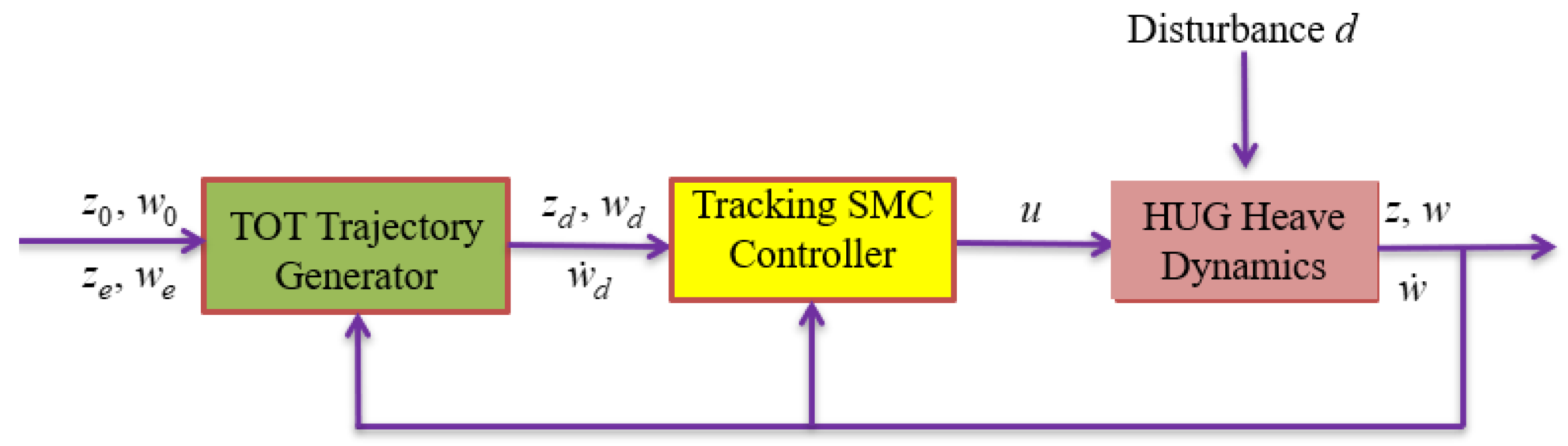
5. Design the Tracking Controller Using the SMC Algorithm

In this section, we introduce the design of a tracking controller for the proposed TOT of the HUG’s depth motion, utilizing the SMC algorithm. The depth trajectory tracking control is depicted in the control system block diagram illustrated in Figure 3. Employing this control strategy ensures the HUG is efficiently guided to the desired depth.

The heave dynamics can be reviewed as follows:

$$\begin{gathered} a\dot{w}+b\left|w\right|w=f+d \\ \dot{z}=w \end{gathered}$$

(70)

where $f$ denotes the control input and $d$ represents the bounded disturbance. It is assumed that the nominal values of the hydrodynamic coefficients for the heave dynamics are known, which allows the controller to focus on dealing with the bounded disturbance $d$. To achieve this, an SMC with a saturation function was developed for the heave dynamics, as shown below.

The sliding surface $\mathrm{s}$ is created as a function of depth error and heave velocity error, represented by Equation (71). The weight $\lambda$ is a positive value that determines the relative importance of position and velocity error in the control design.

$$s=\left(w-w_d\right)+\lambda \left(z-z_d\right)$$

(71)

The expression for the control input $f$ is obtained as follows.

$$f=\widehat{b}w\left|w\right|+\widehat{a}{\dot{w}}_d-\lambda \widehat{a}\left(w-w_d\right)-Ksat\left(\frac{s}{\varphi }\right)$$

(72)

where $\widehat{a}$ and $\widehat{b}$ are the assumed nominal values for the system parameters $a$ and $b$, respectively. The boundary layer for the sliding surface is denoted by $\varphi$, and $K$ is a positive gain that affects the rate of convergence to the sliding surface.

$$K={\Delta }_b{w}^2+{\Delta }_a\left|{\dot{w}}_d-\lambda \left(w-w_d\right)\right|+D+\eta a_{max}$$

(73)

where the controller assumes that the magnitude of uncertainty in the parameters $a$ and $b$, represented by ${\Delta }_a$ and ${\Delta }_b$, respectively, is zero. Additionally, $D$ represents the bound of the external disturbance $d$, $\eta$ is a small positive scalar, and $a_{max}$ is the maximum possible value of $a$.

By utilizing the SMC, the TOT tracking control can be designed to be robust against the effects of external bounded disturbance. The subsequent section aims to demonstrate the effectiveness of combining the TOT and SMC approaches in verifying the tracking performance.

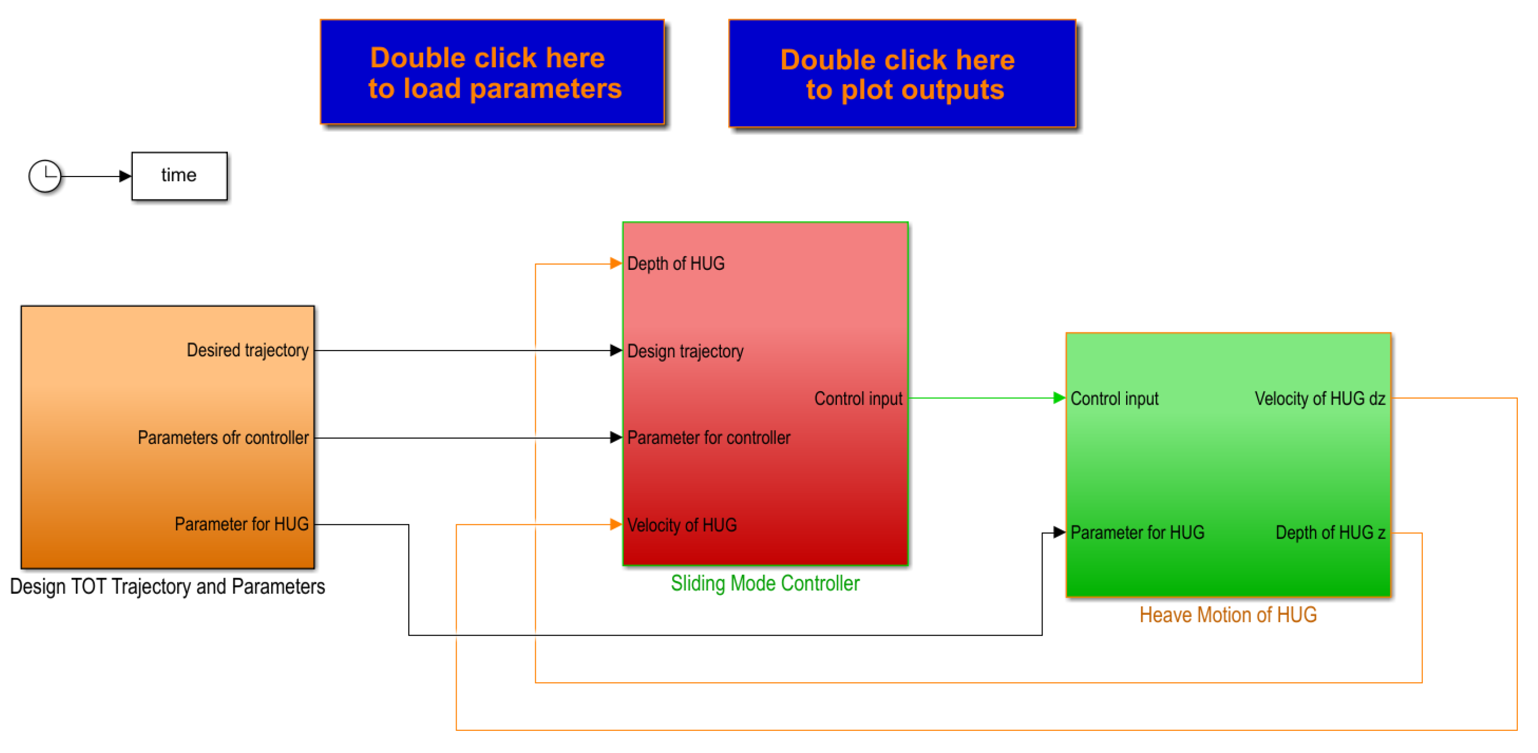
6. Simulation and Discussion

To assess the TOT’s performance and its control input, we conduct a tracking control analysis for the HUG using the SMC algorithm and develop a simulator based on a HUG model. The simulation is implemented using a Matlab-Simulink model comprising three subsystems: one for the designed TOTs and parameters, another for the SMC algorithm, and the third for the heave motion dynamics of the HUG, as illustrated in Figure 4.

Table 2. Parameters for simulation.

$\mathit{D}$ (N)	$\mathit{\eta }$ (m∙s−2)	$\mathit{\lambda }$ (s−1)	$\mathit{\varphi }$ (m∙s−1)	${\mathit{Z}}_{\left|\mathit{w}\right|\mathit{w}}$ (kgm2)	${\mathit{Z}}_{\dot{\mathit{w}}}$ (kgm2)	$\mathit{m}$ (kg)	$\mathit{a}$ (kg)	$\mathit{b}$ (kg)	${\mathit{f}}_{\mathbf{max}}$ (N)	${\mathit{f}}_{\mathbf{min}}$ (N)
2	0.01	2	0.1	0.0356	−0.0119	50.48	50.5	10	3.43	−10

presents the simulation parameters. Simulating the vehicle’s depth control with the proposed TOT and SMC strategy requires utilizing hydrodynamic coefficients and vehicle variables from Vu et al. [29], typically estimated through the CFD method. The values of $a$, $b$, $f_{max}$ (net buoyancy force), and $f_{min}$ (including the thruster force and pitch angle) were set to 50.5 kg, 10 kg, 3.43 N, and −10 N, respectively. Additionally, the rate of buoyancy force, an essential parameter of the buoyancy engine, was assumed to be $c_{max}=-c_{min}=\frac{f_{max}}{20}\mathrm{N}/\mathrm{s}$, and it takes 20 s to reach the maximum force from zero. To further observe the simulation’s performance, we added a disturbance to the dynamics as d = 0.2 sin (2t/π). This disturbance enabled us to test the TOT control input’s ability to oscillate around the predefined input with the same disturbance magnitude. The SMC, which uses a saturation function, was employed in this depth control simulation.

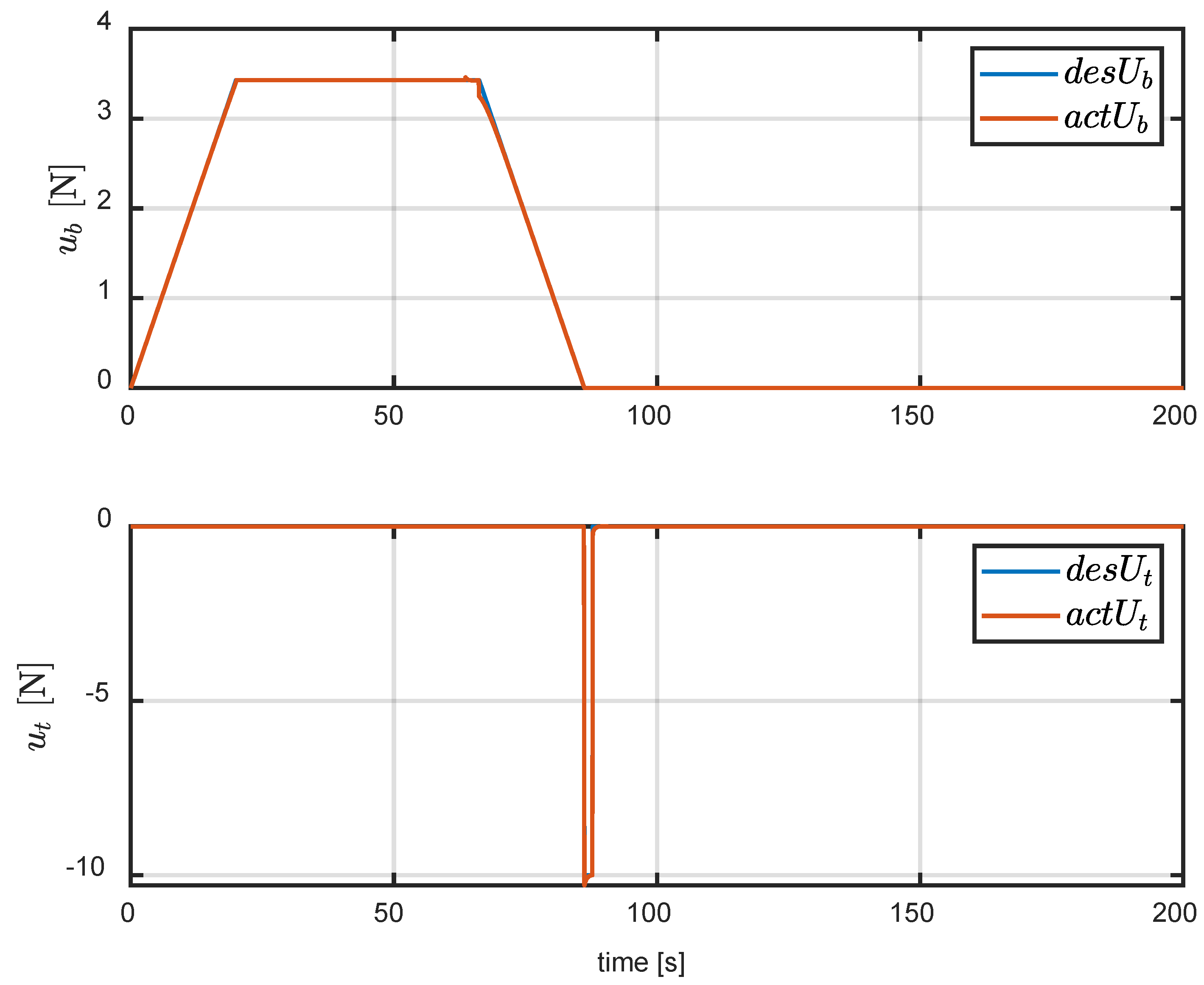
6.1. Simulation 1: Tracking Control of TOT Using SMC Controller without Disturbance

The desired depth for the simulation was set to 40 m, with $z_0=0$ as the water surface and $z_5=40$ m as the target depth. To determine the TOT profile, the times $t_2$, $t_3$, $t_4$, and $t_5$ were obtained using Equations (49), (64), (65), and (69), respectively, resulting in $t_2=63.5238$, $t_3=66.1899$, $t_4=86.1899$, and $t_5=87.7597$. In practical scenarios, the depth $z_3$ at which the buoyancy force must be reversed is crucial to approach the desired depth $z_5$ in a neutral buoyancy condition. By using Equation (63), depth $z_3$ was computed as 30.1475 m for this simulation. Hence, by reversing the buoyancy force at $z_3=30.1475$ m, the HUG vehicle could achieve the target depth $z_5=40$ m in the neutral buoyancy condition.

According to the results depicted in Figure 5, the TOT was accurately tracked by the actual position, velocity, and acceleration. The heave velocity, as illustrated in Figure 5, achieved its maximum value of 0.587 m/s at $t_2$. Meanwhile, the heave acceleration initially increased from zero to 0.031 m/s² and then decreased to zero at $t_2$. From $t_2$ to $t_4$, the net buoyancy force declined to zero to achieve neutral buoyancy, and the thruster was utilized from $t_4$ to $t_5$. During this period, the buoyancy force decreased from 3.43 N to 0 N in 20 s, resulting in a reduction in heave velocity and heave acceleration to 0.32 m/s and −0.22 m/s², respectively. The thruster was responsible for reducing the velocity and acceleration to zero at $t_5$, as shown in Figure 5. After a brief period of operation, the control input of the thruster was set to zero and remained so. As a result, the vehicle’s depth was maintained at 40 m using a 3.43 N buoyancy force and −10 N thrust, with a minimum time of 87.8 s. This simulation can be utilized by designers to verify if their buoyancy engine and thruster force capacity designs meet specific requirements for settling time.

Between time points $t_4$ and $t_5$, the sudden shift in acceleration and velocity trajectories led to a notable spike in the tracking error. Specifically, the position error and velocity error reached levels of $5\times {10}^{-4}$ m and $2\times {10}^{-3}$ m/s, respectively. However, toward the end of the TOT period, all tracking errors gradually subsided and eventually reached zero, as depicted in Figure 6.

As illustrated in Figure 7, the implemented control input closely resembled the pre-planned input. Assuming that the heave dynamics parameters of the actual system match those used in the experiment, utilizing the TOT for control input would push the buoyancy engines and thrusters to their operational limits. By utilizing the full force of these components, it was possible to achieve the shortest possible arrival time for depth control.

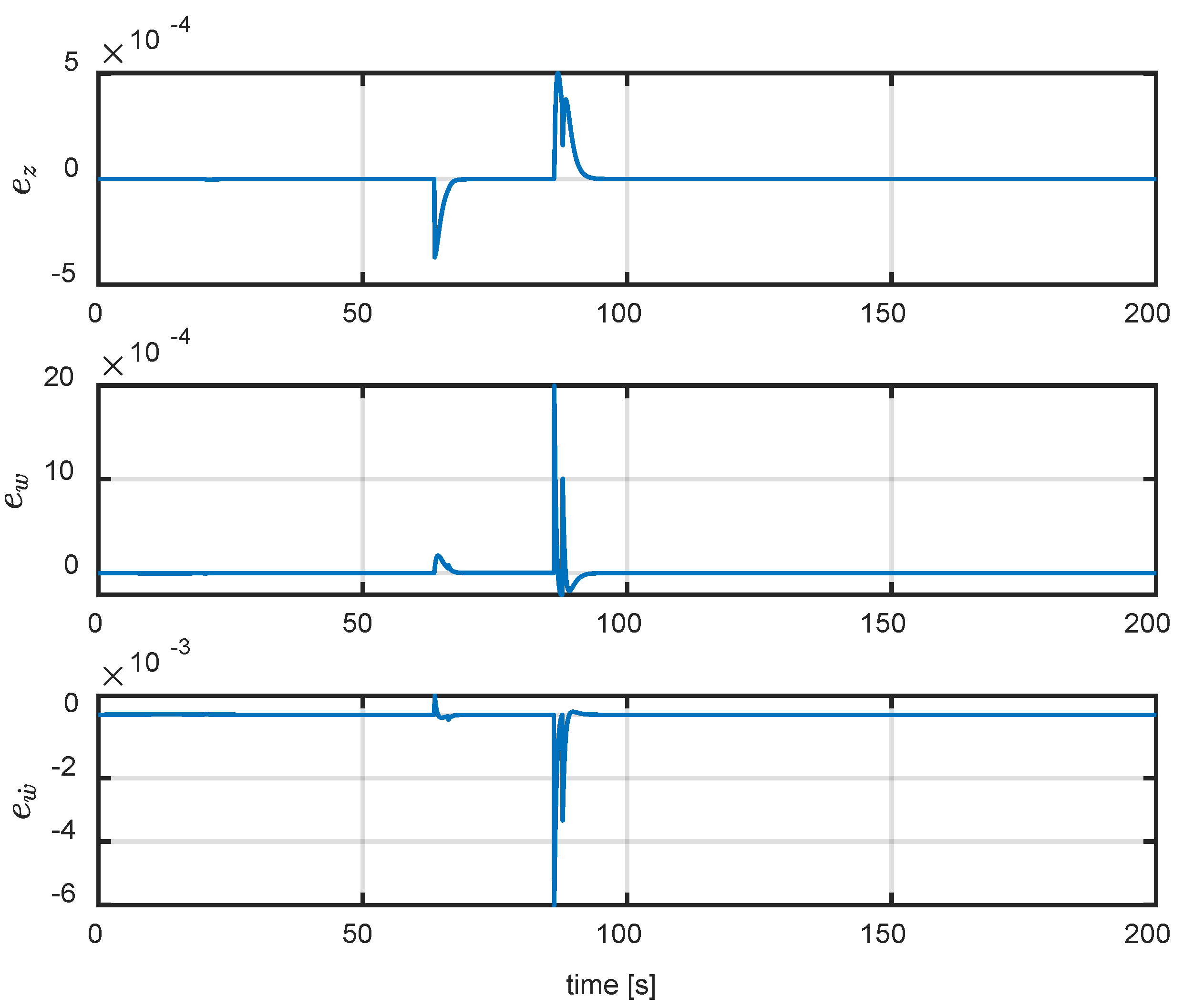
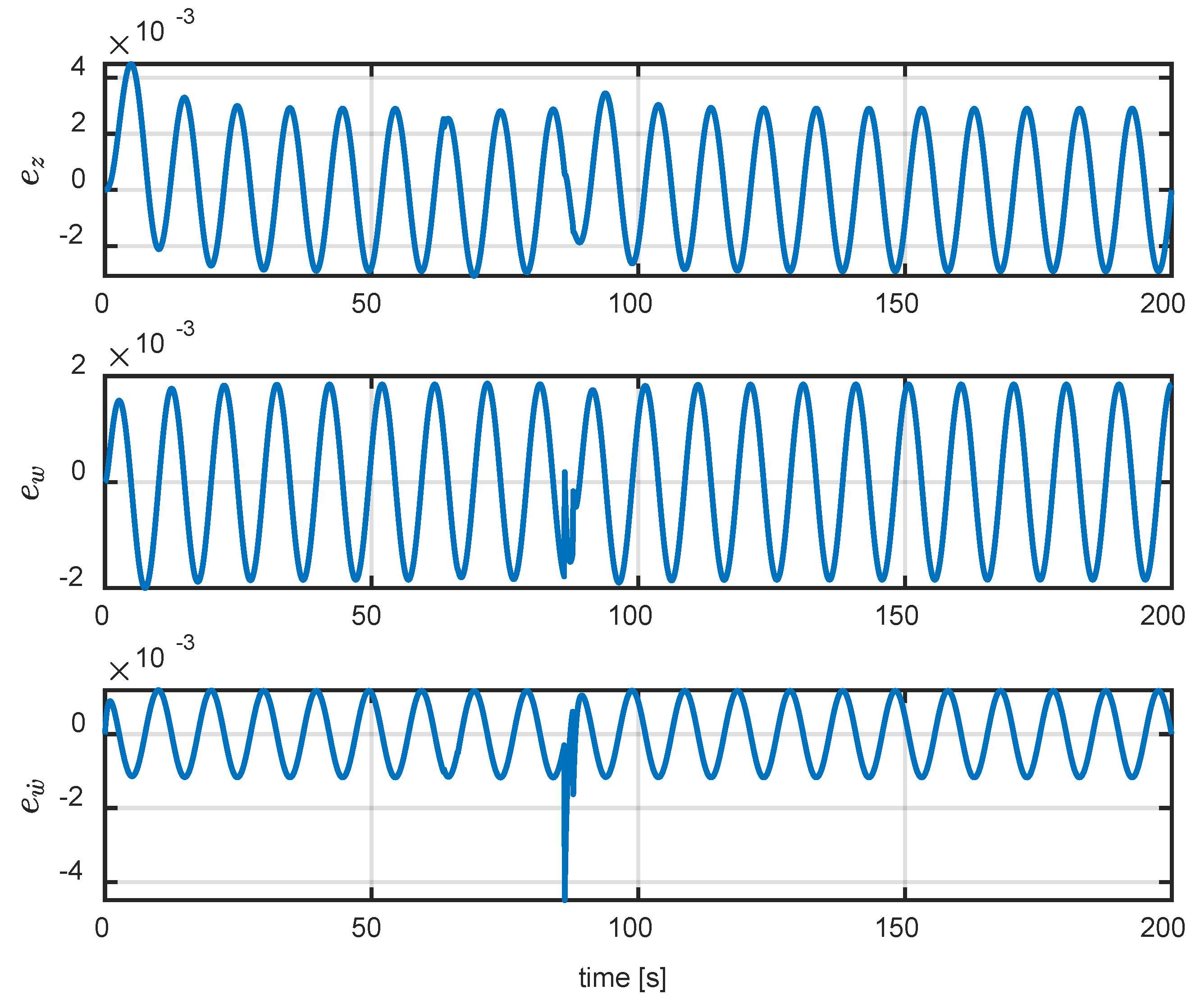
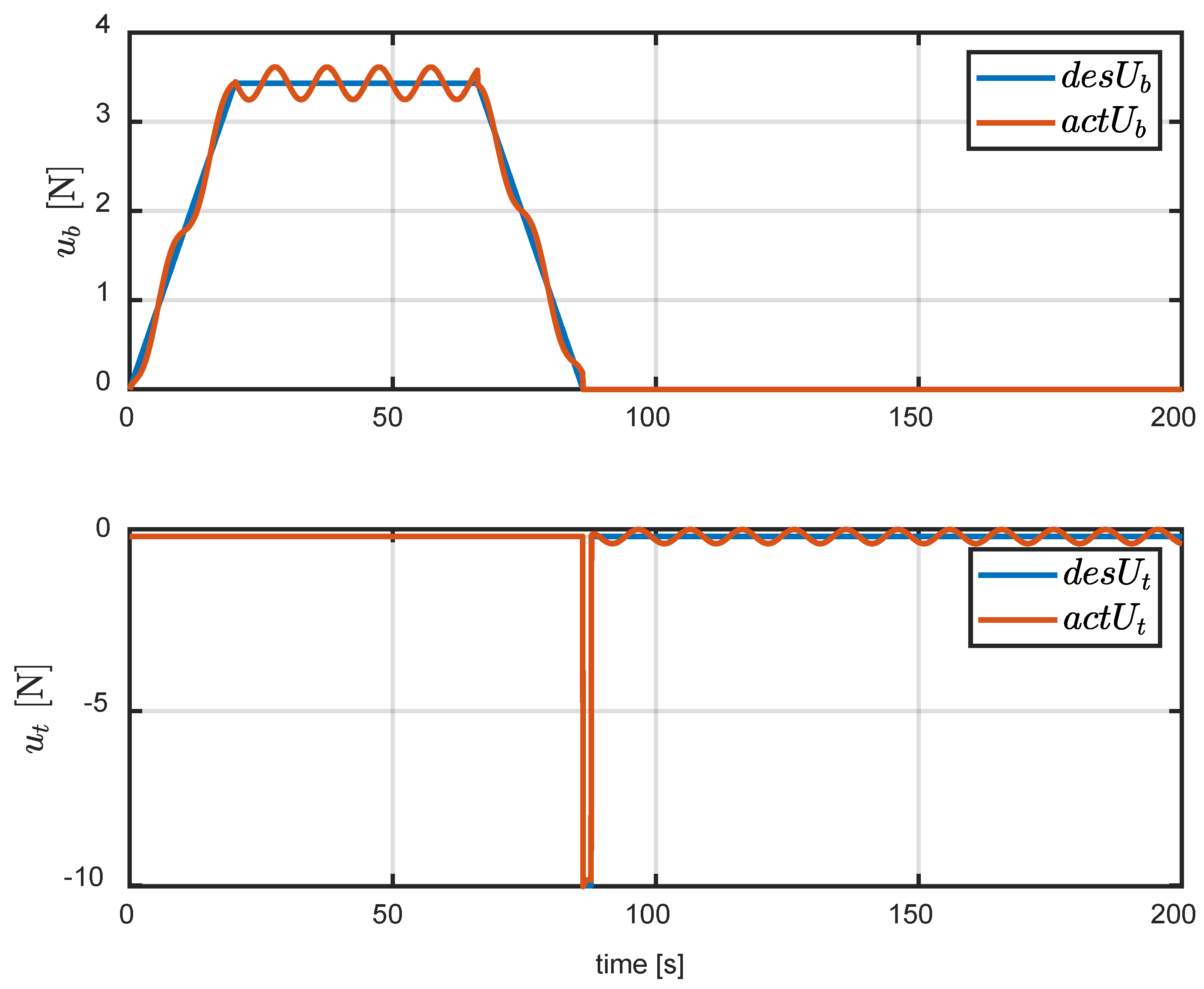
6.2. Simulation 2: Tracking Control of TOT Using SMC Controller under External Disturbance

To evaluate the system’s resilience to external disturbances, we introduced a sinusoidal disturbance (d = 0.2 sin (2t/π)) into the heave dynamics via Equation (2). Despite the presence of the disturbance, the TOT tracking performance remained satisfactory, as depicted in Figure 8. However, due to the chattering elimination using the saturation function in SMC, the tracking error deteriorated slightly, as shown in Figure 9. Even so, the position error remained within 0.002 m, while the velocity error and acceleration error were both controlled below 0.002 m/s and 0.006 m/s², respectively.

Figure 10 illustrates the most crucial result of the simulation, where the control input oscillated around the pre-defined input for the TOT due to the disturbance. Moreover, the magnitude of the actual input deviation was equivalent to that of the disturbance. Specifically, the buoyancy force in this simulation fluctuated between 3.22 N and 3.64 N, while the desired input was 3.43 N, as depicted in Figure 10. However, the average value of the actual buoyancy force was estimated to be 3.43 N, which corresponded to the pre-defined input, with a deviation of 0.2 N, equivalent to the magnitude of the disturbance d = 0.2 sin (2t/π). Figure 10 shows the same phenomenon for the thrusting force after completing the TOT. These results suggest that the magnitude of the disturbance must be factored into the buoyancy engine’s design capacity to ensure proper functioning.

The proposed TOT-based depth control algorithm demonstrated robustness against external bounded disturbances, as shown in simulations. This was achieved through the implementation of a robust SMC strategy, incorporating a saturation function to keep the tracking error minimal under such conditions. The control effort closely followed the desired input, and its deviation was equivalent to the disturbance bound. Overall, the TOT-based approach offers a promising solution for robust depth control in the presence of disturbances.

7. Conclusions

The study developed an analytical solution for the TOT in heave dynamics by utilizing a hybrid actuation scheme that incorporated individual buoyancy and thruster forces. It was assumed that the nominal value of the heave dynamics parameters could be estimated; therefore, the analytical solution of heave dynamics could be formulated using the thrusting saturation and constant buoyancy force rate. Then, the shortest trajectory for depth control of a HUG could be established while considering the actuator saturation. The results of the closed-form heave dynamics solution for the buoyancy engine not only shows the TOT for depth control but also provides a formula to compute the depth for reversing the buoyancy force in practical applications. Once the nominal value of the vehicle mass, added mass, and damping coefficients are defined, the proposed TOT helps the HUG reach the desired depth within the shortest arrival time.

The proposed TOT-based robust depth control algorithm was validated in simulations and demonstrated excellent tracking performance even in the presence of bounded disturbances. According to the simulation results, buoyancy and thruster force were used at the maximum and minimum values; therefore, the consuming time in the depth control was the fastest at around 88 s from 0 m to 40 m depth under the assumption that the system parameters and actuator saturations are defined.

The focus of this study was to design the TOT for the HUG system using the buoyancy engine and thruster. Parameter uncertainties were not taken into account in this analysis. However, if the estimation errors of uncertain system parameters are defined as bounded disturbances, the TOT’s application can be extended to uncertain HUG systems. This aspect will be the focus of our future work. Also, to further validate the proposed TOT and robust control algorithm, some experiments will be conducted on a physical HUG system.

References

1. Cui, R.; Zhang, X.; Cui, D. Adaptive sliding-mode attitude control for autonomous underwater vehicles with input nonlinearities. Ocean Eng. 2016, 123, 45–54. [Google Scholar] [CrossRef]
2. Vasilijevic, A.; Bremnes, J.E.; Ludvigsen, M. Remote Operation of Marine Robotic Systems and Next-Generation Multi-Purpose Control Rooms. J. Mar. Sci. Eng. 2023, 11, 1942. [Google Scholar] [CrossRef]
3. Lu, C.; Yang, J.; Leira, B.J.; Chen, Q.; Wang, S. Three-Dimensional Path Planning of Deep-Sea Mining Vehicle Based on Improved Particle Swarm Optimization. J. Mar. Sci. Eng. 2023, 11, 1797. [Google Scholar] [CrossRef]
4. Von Benzon, M.; Sørensen, F.F.; Uth, E.; Jouffroy, J.; Liniger, J.; Pedersen, S. An Open-Source Benchmark Simulator: Control of a BlueROV2 Underwater Robot. J. Mar. Sci. Eng. 2022, 10, 1898. [Google Scholar] [CrossRef]
5. Vu, M.T.; Thanh, H.L.N.N.; Huynh, T.T.; Do, Q.T.; Do, T.D.; Hoang, Q.D.; Le, T.H. Station-Keeping Control of a Hovering Over-Actuated Autonomous Underwater Vehicle Under Ocean Current Effects and Model Uncertainties in Horizontal Plane. IEEE Access 2021, 9, 6855–6867. [Google Scholar] [CrossRef]
6. Tang, S.; Xue, N.; Lui, K.; Wang, D.; Ye, J.; Fan, T. Motion control for an open-frame work-class ROV in current using an adaptive super-twisting disturbance observer. Ocean Eng. 2023, 280, 114723. [Google Scholar] [CrossRef]
7. Vu, M.T.; Choi, H.S.; Thieu, Q.M.N.; Nguyen, N.D.; Lee, S.D.; Le, T.H.; Sur, J. Docking assessment algorithm for autonomous underwater vehicles. Appl. Ocean Res. 2020, 100, 102180. [Google Scholar] [CrossRef]
8. Lv, T.; Wang, Y.; Liu, X.; Zhang, M. Command-Filter-Based Region-Tracking Control for Autonomous Underwater Vehicles with Measurement Noise. J. Mar. Sci. Eng. 2023, 11, 2119. [Google Scholar] [CrossRef]
9. Zhang, J.; Ning, X.; Ma, S. An improved particle swarm optimization based on age factor for multi-AUV cooperative planning. Ocean Eng. 2023, 287, 115753. [Google Scholar] [CrossRef]
10. Deutsch, C.; Kuttenkeuler, J.; Melin, T. Glider performance analysis and intermediate-fidelity modelling of underwater vehicles. Ocean Eng. 2020, 210, 107567. [Google Scholar] [CrossRef]
11. Du, X.; Liu, X.; Song, Y. Analysis of the Steady-Stream Active Flow Control for the Blended-Winged-Body Underwater Glider. J. Mar. Sci. Eng. 2023, 11, 1344. [Google Scholar] [CrossRef]
12. Wu, Q.; Wu, H.; Jiang, Z.; Tan, L.; Yang, Y.; Yan, S. Multi-objective optimization and driving mechanism design for controllable wings of underwater gliders. Ocean Eng. 2023, 286, 115534. [Google Scholar] [CrossRef]
13. Shen, X.R.; Wang, Y.H.; Yang, S.Q.; Liang, Y.; Li, H. Development of underwater gliders: An overview and prospect. J. Unmanned Undersea Syst. 2018, 26, 89–106. [Google Scholar]
14. Yang, M.; Wang, Y.; Chen, Y.; Wang, C.; Liang, Y.; Yang, S. Data-driven optimization design of a novel pressure hull for AUV. Ocean Eng. 2022, 257, 111562. [Google Scholar] [CrossRef]
15. Yang, Y.; Liu, Y.; Wang, Y.; Zhang, H.; Zhang, L. Dynamic modeling and motion control strategy for deep-sea hybrid-driven underwater gliders considering hull deformation and seawater density variation. Ocean Eng. 2017, 143, 66–78. [Google Scholar] [CrossRef]
16. Webb, D.C.; Simonetti, P.J.; Jones, C.P. SLOCUM: An underwater glider propelled by environment energy. IEEE J. Ocean. Eng. 2001, 26, 447–452. [Google Scholar] [CrossRef]
17. Wang, Y.; Bulger, C.; Thanyamanta, W.; Bose, N. A Backseat Control Architecture for a Slocum Glider. J. Mar. Sci. Eng. 2021, 9, 532. [Google Scholar] [CrossRef]
18. Sherman, J.; Davis, R.E.; Owens, W.B.; Valdes, J. The autonomous underwater glider “Spray”. IEEE J. Ocean. Eng. 2001, 26, 437–446. [Google Scholar] [CrossRef]
19. Eriksen, C.C.; Osse, T.J.; Light, R.D.; Wen, T.; Lehman, T.W.; Sabin, P.L.; Ballard, J.W.; Chiodi, A.M. Sea glider: A long range autonomous underwater vehicle for oceanographic research. IEEE J. Ocean. Eng. 2001, 26, 424–436. [Google Scholar] [CrossRef]
20. Anderlini, E.; Harris, C.; Phillips, A.B.; Lopez, A.L.; Woo, M.; Thomas, G. Towards autonomy: A recommender system for the determination of trim and flight parameters for Seagliders. Ocean Eng. 2019, 189, 106338. [Google Scholar] [CrossRef]
21. Osse, T.J.; Eriksen, C.C. The deep glider: A full ocean depth glider for oceanographic research. In Proceedings of the Oceans’07, Vancouver, BC, Canada, 29 September–4 October 2007; pp. 1–12. [Google Scholar]
22. Wang, P.; Wang, X.; Wang, Y.; Niu, W.; Yang, S.; Sun, C.; Luo, C. Dynamics Modeling and Analysis of an Underwater Glider with Dual-Eccentric Attitude Regulating Mechanism Using Dual Quaternions. J. Mar. Sci. Eng. 2023, 11, 5. [Google Scholar] [CrossRef]
23. Jenkins, S.A.; Humphreys, D.E.; Sherman, J.; Osse, J.; Jones, C.; Leonard, N.; Graver, J.; Bachmayer, R.; Clem, T.; Carroll, P.; et al. Underwater Glider System Study (Technical Report 53); Scripps Institution of Oceanography: San Diego, CA, USA, 2003. [Google Scholar]
24. Tian, X.; Zhang, L.; Zhang, H. Research on Sailing Efficiency of Hybrid-Driven Underwater Glider at Zero Angle of Attack. J. Mar. Sci. Eng. 2022, 10, 21. [Google Scholar] [CrossRef]
25. Wu, X.; Yu, P.; Zhang, C.; Wang, Q.; Zhu, Z.; Wang, T. Shape optimization of underwater glider for maximum gliding range with uncertainty factors considered. Ocean Eng. 2023, 287, 115869. [Google Scholar] [CrossRef]
26. Chyba, M.; Leonard, N.E.; Sontag, E.D. Time-Optimal Control for Underwater Vehicles. IFAC Proc. Vol. 2000, 33, 117–122. [Google Scholar] [CrossRef]
27. Chyba, M.; Haberkorn, T.; Smith, R.N.; Choi, S.K. Design and implementation of time efficient trajectories for autonomous underwater vehicles. Ocean Eng. 2008, 35, 63–76. [Google Scholar] [CrossRef]
28. Rhoads, B.; Mezić, I.; Poje, A.C. Minimum time heading control of underpowered vehicles in time-varying ocean currents. Ocean Eng. 2013, 66, 12–31. [Google Scholar] [CrossRef]
29. Vu, M.T.; Choi, H.S.; Kang, J.I.; Ji, D.H.; Joong, H. Energy efficient trajectory design for the underwater vehicle with bounded inputs using the global optimal sliding mode control. J. Mar. Sci. Technol. 2017, 25, 705–714. [Google Scholar]
30. Nguyen, N.D.; Vu, M.T.; Nguyen, P.; Huang, J.; Jung, D.W.; Cho, H.; Phan, H.N.A.; Choi, H.-S. Time-Optimal Trajectory Design for Heading Motion of the Underwater Vehicle. J. Mar. Sci. Eng. 2023, 11, 1099. [Google Scholar] [CrossRef]
31. Koubaa, Y.; Boukattaya, M.; Damak, T. Adaptive sliding mode control for nonholonomic mobile robot with uncertain kinematics and dynamics. Appl. Artif. Intell. 2018, 32, 924–938. [Google Scholar] [CrossRef]
32. Vu, M.T.; Van, M.; Bui, D.H.P.; Do, Q.T.; Huynh, T.T.; Lee, S.D.; Choi, H.S. Study on Dynamic Behavior of Unmanned Surface Vehicle-Linked- Unmanned Underwater Vehicle System for Underwater Exploration. Sensors 2020, 20, 1329. [Google Scholar] [CrossRef]
33. Vu, M.T.; Le, T.H.; Thanh, H.L.N.N.; Huynh, T.T.; Van, M.; Hoang, Q.D.; Do, Q.T. Robust Position Control of an Over-actuated Underwater Vehicle under Model Uncertainties and Ocean Current Effects Using Dynamic Sliding Mode Surface and Optimal Allocation Control. Sensors 2021, 21, 747. [Google Scholar] [CrossRef] [PubMed]
34. Zhang, X.; Zhou, H.; Fu, J.; Wen, H.; Yao, B.; Lian, L. Adaptive integral terminal sliding mode based trajectory tracking control of underwater glider. Ocean Eng. 2023, 269, 113436. [Google Scholar] [CrossRef]
35. Zhang, W.; Wu, W.; Li, Z.; Du, X.; Yan, Z. Three-Dimensional Trajectory Tracking of AUV Based on Nonsingular Terminal Sliding Mode and Active Disturbance Rejection Decoupling Control. J. Mar. Sci. Eng. 2023, 11, 959. [Google Scholar] [CrossRef]
36. Sahu, B.K.; Subudhi, B. Adaptive tracking control of an autonomous underwater vehicle. Int. J. Autom. Comput. 2015, 11, 299–307. [Google Scholar] [CrossRef]
37. Li, J.H.; Lee, P.M. Design of an adaptive nonlinear controller for depth control of an autonomous underwater vehicle. Ocean Eng. 2005, 32, 2165–2181. [Google Scholar] [CrossRef]
38. Park, B.S.; Kwon, J.-W.; Kim, H. Neural network-based output feedback control for reference tracking of underactuated surface vessels. Automatica 2017, 77, 353–359. [Google Scholar] [CrossRef]
39. Chiman, K.; Lewis, F.L. Robust backstepping control of nonlinear systems using neural networks. IEEE Trans. Syst. Man. Cybernetics 2000, 30, 753–766. [Google Scholar]
40. Thanh, H.L.N.N.; Vu, M.T.; Mung, N.X.; Nguyen, N.P.; Phuong, N.T. Perturbation Observer-Based Robust Control Using a Multiple Sliding Surfaces for Nonlinear Systems with Influences of Matched and Unmatched Uncertainties. Mathematics 2020, 8, 1371. [Google Scholar] [CrossRef]
41. Li, J.; Du, J.; Chang, W.-J. Robust time-varying formation control for underactuated autonomous underwater vehicles with disturbances under input saturation. Ocean Eng. 2019, 179, 180–188. [Google Scholar] [CrossRef]
42. Liang, X.; Qu, X.; Wang, N.; Zhang, R.; Li, Y. Three-dimensional trajectory tracking of an underactuated AUV based on fuzzy dynamic surface control. IET. Intell. Transp. Syst. 2019, 14, 364–370. [Google Scholar] [CrossRef]
43. Zhong, Y.; Yang, Y.; He, K.; Chen, C. Fast terminal sliding-mode control based on unknown input observer for the tracking control of underwater vehicles. Ocean Eng. 2022, 264, 112480. [Google Scholar] [CrossRef]
44. Rojsiraphisal, T.; Mobayen, S.; Asad, J.H.; Vu, M.T.; Chang, A.; Puangmalai, J. Fast Terminal Sliding Control of Underactuated Robotic Systems Based on Disturbance Observer with Experimental Validation. Mathematics 2021, 9, 1935. [Google Scholar] [CrossRef]
45. Claus, B.; Bachmayer, R.; Cooney, L. Analysis and development of a buoyancy-pitch based depth control algorithm for a hybrid underwater glider. In Proceedings of the 2012 IEEE/OES Autonomous Underwater Vehicles (AUV), Southampton, UK, 24–27 September 2012; pp. 1–6. [Google Scholar]
46. Fossen, T.I. Guidance and Control of Ocean Vehicles; John Wiley & Sons: New York, NY, USA, 1994. [Google Scholar]
47. Fossen, T.I. Handbook of Marine Craft Hydrodynamics and Motion Control; John Wiley & Sons: Hoboken, NJ, USA, 2011. [Google Scholar]
Figure 1. Buoyancy engine and thruster location in the HUG system.
Jmse 11 02216 g001
Figure 2. The profile of the proposed TOT: (a) force, (b) position, (c) velocity, and (d) acceleration.
Jmse 11 02216 g002
Figure 3. HUG depth control scheme sliding mode control algorithm.
Jmse 11 02216 g003
Figure 4. Simulation program.
Jmse 11 02216 g004
Figure 5. Tracking control performance of TOT using SMC controller without disturbance.
Jmse 11 02216 g005
Figure 6. Tracking error of TOT using SMC controller without disturbance.
Jmse 11 02216 g006
Figure 7. Control input of buoyancy engine and thruster for tracking the TOT without disturbance.
Jmse 11 02216 g007
Figure 8. Tracking control performance of TOT using SMC controller with disturbance.
Jmse 11 02216 g008
Figure 9. Tracking error of TOT using SMC controller with disturbance.
Jmse 11 02216 g009
Figure 10. Control input of buoyancy engine and thruster for tracking the TOT with disturbance.
Jmse 11 02216 g010