Developing Functional Recharge Systems to Control Saltwater Intrusion via Integrating Physical, Numerical, and Decision-Making Models for Coastal Aquifer Sustainability

Abstract

Controlling the hydraulic heads along a coastal aquifer may help to effectively manage saltwater intrusion, improve the conventional barrier’s countermeasure, and ensure the coastal aquifer’s long-term viability. This study proposed a framework that utilizes a decision-making model (DMM) by incorporating the results of two other models (physical and numerical) to determine proper countermeasure components. The physical model is developed to analyze the behavior of saltwater intrusion in unconfined coastal aquifers by conducting two experiments: one for the base case, and one for the traditional vertical barrier. MODFLOW is used to create a numerical model for the same aquifer, and experimental data are used to calibrate and validate it. Three countermeasure combinations, including vertical barrier, surface, and subsurface recharges, are numerically investigated using three model case categories. Category (a) model cases investigate the hydraulic head’s variation along the aquifer to determine the best recharge location. Under categories (b) and (c), the effects of surface and subsurface recharges are studied separately or in conjunction with a vertical barrier. As a pre-set of the DMM, evaluation and classification ratios are created from the physical and numerical models, respectively. The evaluation ratios are used to characterize the model case results, while the classification ratios are used to classify each model case as best or worst. An analytical hierarchy process (AHP) as a DMM is built using the hydraulic head, salt line, repulsion, wedge area, and recharge as selection criteria to select the overall best model case. According to the results, the optimum recharging location is in the length ratio (LR) from 0.45 to 0.55. Furthermore, the DMM supports case3b (vertical barrier + surface recharge) as the best model case to use, with a support percentage of 48%, implying that this case has a good numerical model classification with a maximum repulsion ratio (R_r) of 29.4%, and an acceptable wedge area ratio (WAR) of 1.25. The proposed framework could be used in various case studies under different conditions to assist decision-makers in evaluating and controlling saltwater intrusion in coastal aquifers.

1. Introduction

Due to the natural effects of long-term climate change, such as sea level change and tidal intensity fluctuations, seawater flows toward freshwater aquifers. In addition, increased water demands accompanied by anthropogenic activities such as excessive pumping of freshwater in coastal areas cause the lowering of water tables as well as saltwater intrusion [1,2]. Saltwater intrusion lowers the availability and quality of freshwater in coastal regions, as reported at many locations all over the world [3,4,5,6,7,8,9,10,11]. Therefore, it is important to control saltwater intrusion with efficient countermeasures to achieve sustainable freshwater sources.

1.1. Traditional Saltwater Intrusion Countermeasures

Traditional methods for controlling saltwater intrusion include reducing pumping rates, relocating pumping wells, changing pumping patterns, constructing physical subsurface barriers, and saltwater abstraction [10,12,13,14,15,16]. The limitations and high costs of the aforementioned methods pose substantial challenges to their implementation.

1.2. Artificial Groundwater Recharge

Artificial recharge techniques can be used for establishing hydraulic barriers to mitigate saltwater intrusion while recovering SGD [17,18,19]. These techniques have several advantages compared to traditional methods, including low cost, no inundation storage space, less water evaporation, and improved water quality [20]. Although artificial recharge has numerous advantages, it also has disadvantages, including groundwater contamination from surface water, difficulty in implementation due to a lack of understanding of aquifer hydrogeological properties, the potential for environmental damage and soil disturbance, and high maintenance costs [21]. Surface recharge systems include ditches and furrows, recharge basins, stream augmentation, and runoff conservation structures (terracing, contour bunds, percolation tanks, gully plugs, Nalah bunds, and check dams) [22,23,24]. On the other hand, subsurface recharge systems include subsurface injection wells, borewells, and recharging pits and shafts [24,25,26]. Combining traditional and artificial recharge techniques is one way to overcome the disadvantages of both. Although many studies investigate saltwater intrusion in coastal aquifers, only a limited number study the control methods of saltwater intrusion [27,28].

1.3. Integrating Physical and Numerical Models

Physical and numerical models have not only proven to be more effective tools for selecting the optimum solutions for controlling saltwater intrusion but they can also be used to reduce the need for expensive hydrogeological and environmental investigations before constructing a full-scale project [1,29,30,31,32,33,34,35].

Although physical and numerical models are useful in determining the optimum solutions for controlling saltwater intrusion, deficiencies in the acquisition of appropriate evidence to support the final decision are discovered. Since the scenarios of hydrogeological models for a specific aquifer cannot agree on minimizing intrusion, improving groundwater availability, being environmentally friendly, and being cost-effective, it is necessary to use decision models in conjunction with physical and numerical models to guide stakeholders toward sustainable resource management based on a set of criteria.

1.4. Analytical Hierarchy Process (AHP)

The analytical hierarchy process (AHP) is a decision-making method that has been used alone or in conjunction with other techniques such as GIS and fuzzy logic in a variety of groundwater-related fields. Based on a broader set of criteria, this technique is used to guide stakeholders involved in groundwater development and sustainable resource management [36,37]. The applications of AHP in the field of groundwater include assessing groundwater vulnerability by developing indices based on hydrogeological parameters and mapping groundwater potential zones [38,39,40,41,42,43,44,45,46,47,48]. In the field of saltwater intrusion, a GIS-based AHP weighted index overlay analysis technique has been demonstrated to determine the distribution of groundwater vulnerability [49,50]. A fuzzy-AHP evaluation model is developed for analyzing the level of seawater intrusion in long-term monitoring data from multiple river basins [50]. The AHP is also used to compute weights for the GALDIT parameters, which are used to assess the vulnerability of coastal aquifers to saltwater intrusion [51].

In the study, according to the preceding overview, both traditional and artificial techniques of controlling seawater intrusion have limitations, and using physical, numerical, and decision-making models is crucial. The unconfined coastal aquifer is investigated in this study, and physical, numerical, and decision-making models are utilized to investigate surface and subsurface recharge methods, either alone or in combination with typical vertical barriers. On the other hand, the behaviors of saltwater intrusion, groundwater flow, and hydraulic head are numerically investigated using three categories of model cases: categories (a), (b), and (c). Category (a) model cases explore the variation in hydraulic head along the aquifer in order to determine the appropriate recharging location. The impacts of surface and subsurface recharges are explored separately or in conjunction with a vertical barrier in categories (b) and (c). The aims of this study are: (i) To examine experimentally the behavior of saltwater intrusion via coastal unconfined aquifers with and without vertical barrier countermeasures; (ii) To develop a validated numerical model regarding the experimental findings of transitory saltwater intrusion; (iii) To identify the optimal recharging location utilizing the location of the minimum hydraulic head; (v) To determine the optimal vertical barrier depth for saltwater intrusion management; (iv) To identify the components of an effective countermeasure system, such as a vertical barrier, surface recharge, and subsurface recharge, either alone or in combination; (vi) To develop a DMM model to aid decision-makers in the selection among several saltwater countermeasures and picking the most appropriate one depending on various demanding scenarios.

2. Materials and Methodologies

Although it is challenging to identify specific locations with entirely homogeneous coastal aquifers, some regions may exhibit relatively homogeneous aquifers compared to others. The Florida Keys in the United States are primarily composed of limestone, which can exhibit more uniform hydrogeological properties compared to other types of geological formations [52,53]. The coastal aquifers in parts of Senegal, West Africa, are known for their relatively uniform properties, owing to the prevalence of specific geological formations, such as sand and sandstone, which contribute to more consistent hydrogeological behavior [54]. The Eastern Shore of Maryland has been recognized for its relatively homogeneous aquifers due to the prevalence of sedimentary formations, particularly the Columbia and Calvert aquifers, which are known for their relatively uniform properties [55]. Certain areas along the northern coast of the Black Sea in Russia are known for their relatively homogeneous coastal aquifers, largely attributed to the dominance of specific sedimentary formations and the uniformity of underlying geological structures [56].

In this study, saltwater intrusion is investigated experimentally by developing a laboratory physical model of a homogeneous unconfined coastal aquifer. Two experiments are carried out in this part, and dimensionless quantities are formed, namely evaluation ratios. These evaluation ratios are used to analyze and characterize the saltwater line and hydraulic head variations of the numerical model cases, as forthcoming later. A numerical finite difference model is created, and the validation and calibration processes are carried out using the experimental results. Following that, numerical methods are utilized to investigate how to control saltwater intrusion, taking into account the combined effect of using vertical barriers with surface or subsurface recharge systems, as demonstrated by model cases divided into three categories (a, b, and c), each with seven cases. Category (a) model cases are used to determine the location of the minimal hydraulic heads, which are suggested to be the locations of the indicated artificial recharge systems. Categories (b) and (c) investigate the impacts of surface and subsurface recharges on saltwater intrusion at the indicated locations, either alone or in conjunction with a vertical barrier. A classification process is then implemented to classify model cases in each category as the best or worst model case using a developed set of ratios, namely classification ratios. Because each model case is expected to have benefits and drawbacks, as well as several criteria governing the model cases, the benefits and drawbacks of each model case should be quantified in order to identify the most effective one. Following that, the most effective model case is decided on using a new DMM model based on the AHP technique. To make the final decision, two selection levels (levels 1 and 2) are considered. Level 1 is used to select the best model case from each category (three model cases), while level 2 is utilized for selecting the best overall model case. Figure 1 illustrates a flow chart for the framework of the study.

2.1. Experimental Setup

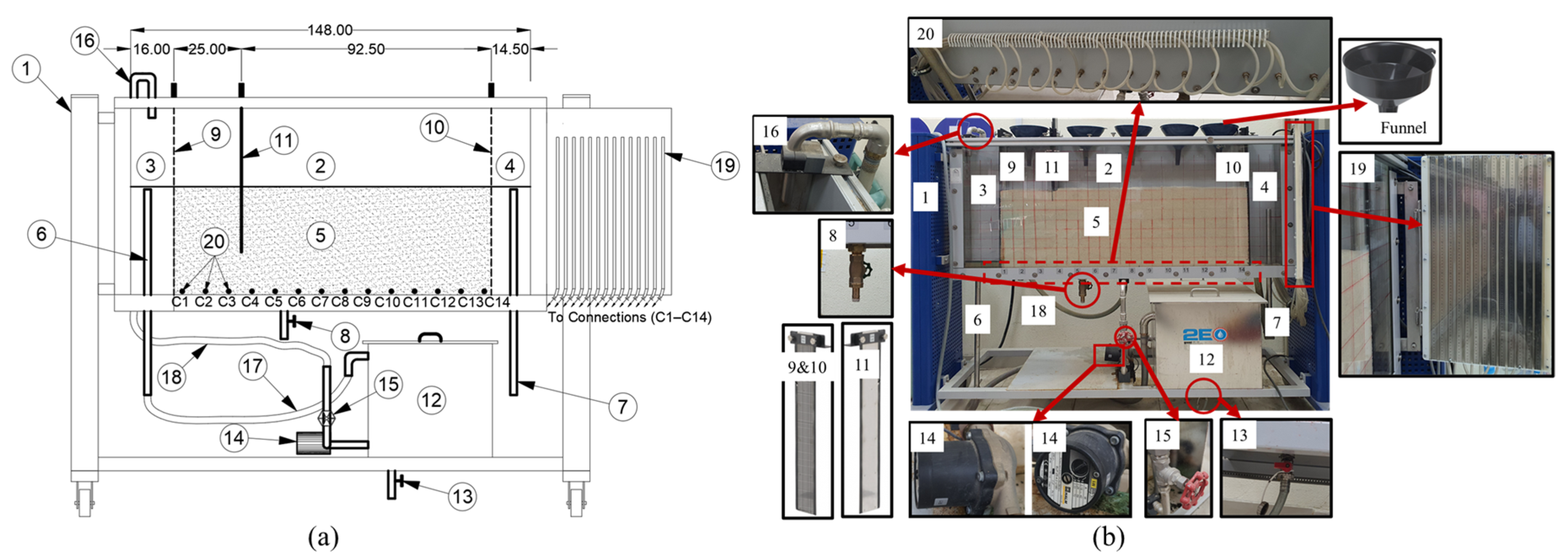
2.1.1. Drainage and Seepage Tank (DS Tank)

The DS Tank is used in this study to visualize groundwater flow through permeable porous media. The model of the DS tank that is used in the current study is HM 169 GUNT HAMBURG [57]. The DS tank consists of a porous media container, a lower water tank as a water source, a pump for the water flow, a valve to adjust the water supply, and measuring connections in the experimental section, which are connected to 14 glass tube manometers to display and measure hydraulic heads along the DS Tank. The sand container consists of an aluminum rectangular tank with a transparent front side (methacrylate material) to visualize groundwater flow and optimize observation of the experiments through the porous media. In the DS Tank, two fine mesh screens are used to create feed and discharge chambers and to separate the experimental section from these two chambers. There are two adjustable overflow pipes in the DS Tank for adjusting the water levels in the mentioned chambers and measuring the water flow. To prevent seawater intrusion, an aluminum sheet pile is used as a vertical barrier. As a result, the DS Tank has a closed water circuit with a storage tank and pump. The DS Tank and its components are depicted in Figure 2 and

Table 1. DS Tank components and descriptions.

No.	Component Name	Description	No.	Component Name	Description
1	Steel frame	The DS Tank’s frame	11	Vertical aluminum sheet pile	Vertical barrier to control saltwater intrusion
2	Experimental section	Tank with porous media for monitoring saltwater intrusion	12	Storage tank	The primary source of seawater
3	Feed Chamber	Source of saltwater	13	Draining pipe2	Before the next experiment, drain the saltwater from the storage tank.
4	Discharge Chamber	Source of freshwater	14	Pump	Pumping saltwater to the feed chamber
5	Porous media	Silica sand (0.71–1.18 mm)	15	Pump valve	Pump flow rate adjustment
6	Outflow pipe1	Changing the saltwater level in the feed chamber	16	Saltwater inflow pipe	Connecting with a pump to allow saltwater to flow from the pump to the feed chamber
7	Outflow pipe2	Changing the level of freshwater in the discharge chamber	17	Hose1	Connecting the outflow pipe1 to the storage tank
8	Draining pipe1	Before beginning a new experiment, drain the water from the experimental section.	18	Hose2	Linking the saltwater inflow pipe to the pump
9	Vertical screen1	Separating the feed chamber from the experimental section	19	14 glass manometer tubes	Hydraulic head monitoring along the experimental section
10	Vertical screen2	Separating the discharge chamber from the experimental section	20	Measuring connections	Linked to the 14 glass manometer tubes

.

2.1.2. Configuration and Experimental Set

The DS tank and the associated materials, including saltwater, freshwater, and porous media, are pre-set for the experiments. A horizontal and vertical scale of 5 cm × 5 cm is drawn on the transparent front side of the DS tank, as shown in Figure 3. The left chamber is configured as a saltwater feed chamber with a width of 16 cm. The right chamber is configured as a freshwater discharge chamber with a width of 14.5 cm. Vertical screen barriers separate the experimental section of the DS tank (length 117.5 cm) from the feed and discharge chambers. The experimental section is filled to a depth of 40 cm with porous media soil (graded silica sand with grain sizes ranging from 0.71 to 1.18 mm (see Figure 3). The filling process is done in layers of 5 cm each, with a falling height of 50 cm for each layer, to ensure a homogeneous hydrogeological property of the media sand. In the filling process, funnels are used, which are distributed along the experimental section as shown in Figure 2b.

The seawater used in the experiments is collected from the Red Sea, and its density, as well as that of the freshwater, is calibrated using a sensitive scale and a standard flask (see Figure 4). According to the calibration, the densities of saltwater and freshwater are 0.99 and 1.022 g/cm³, respectively. In saltwater, a 0.15 g/L concentration of green food dye is used to easily visualize the saltwater line and measure the intrusion distance inside the media sand (see Figure 3).

2.1.3. Experimental Procedures

The experiment procedures include the following five steps:

• Freshwater saturation of the media sand: At the start of the experiment, the outflow pipes1 and 2 for both the feed and discharge chambers are set to be at the same level as the media sand surface (40 cm from the DS Tank bed). Following that, freshwater is discharged at a constant rate into both chambers until the media sand in the experimental section is saturated. The hydraulic heads along the experimental section are monitored by the 14 glass tube manometers until the water level reaches the sand surface in all the manometers to verify the saturation condition.
• Feeding the experiment with colored saltwater: In the feed chamber, an aluminum sheet pile is used to block water seepage through the experimental section. Following that, the feed chamber’s outflow pipe1 is moved to the DS Tank bed level to empty it of freshwater. The outflow pipe is then returned to its previous level (media sand surface level), and the storage tank is subsequently emptied and filled with the green-dyed saltwater. When the pump is turned on and the pump valve is opened, saltwater begins to fill the feed chamber all the way to the top of the outflow pipe1. Following that, the pump valve is manually adjusted to maintain the saltwater level at the surface of the media sand.
• Adjusting the water levels in the feed and discharge chambers: The first step in this process is to remove the aluminum sheet pile from the feed chamber. Furthermore, to achieve a suitable flow through the media sand, the difference in water levels between the feed and discharge chambers is tested several times and finally adjusted to 10 cm, resulting in a hydraulic gradient of 0.085. To accomplish this, the outflow pipe2 for the discharge chamber is adjusted to be 10 cm below the media sand surface.
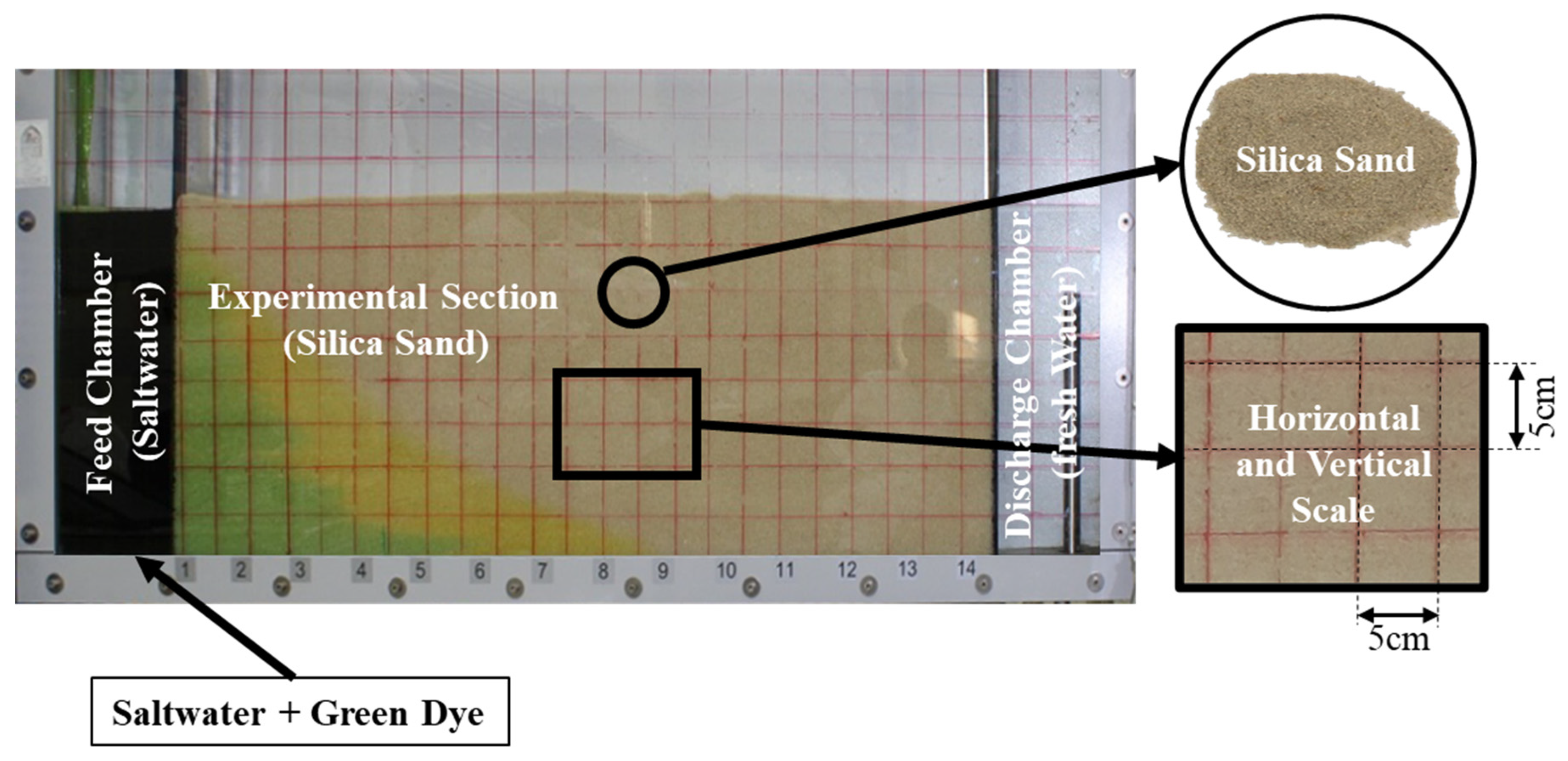
• Monitoring of saltwater intrusion: In the experimental section, saltwater begins to infiltrate through the media sand and can be observed through the transparent front side of the DS Tank. The temporal saltwater intrusion could be measured using the horizontal and vertical scales drawn on the transparent front side. The saltwater intrusion is measured at 30 min intervals. Photos for each time interval are taken with a high-resolution digital camera and used to validate the observed saltwater lines with AutoCAD software (Version S.51.0.0 AutoCAD 2022). During the experiment, the freshwater level inside the discharge chamber rises until it reaches its maximum level by adjusting the outflow pipe2 level above the media sand surface level until it reaches a steady state.

This experimental part of the study considers two experiments:

Experiment 1 (Base Case): This is the case in which the saltwater intrusion through the media sand is studied without any countermeasures. In this case, the procedures from steps 1 to 4 are carried out.

Experiment 2 (using a vertical barrier): Through this experiment, the media sand is removed from the experimental section. Then, the vertical aluminum sheet pile (vertical barrier) is used as a countermeasure against saltwater intrusion and placed in the experimental section, 25 cm from the feed chamber. Hereafter, media sand is refilled in the experimental section. The penetration depth of the vertical aluminum sheet pile is set below the silica sand surface by a depth of 30 cm. Then, the steps from 1 to 4 are implemented.

2.2. Evaluation Ratios

Based on the geometry and experiment design given in the preceding section, Figure 5 and

Table 2. Definition of the geometric characteristics of the experiments.

No.	Quantity	Type			Definition
		Constant	Parameter	Variable
1	Hsw	√			Hydraulic head of the saltwater boundary
2	D	√			Sand media depth
3	Lmedia	√			Sand media length (experimental section length)
4	max.L(in)	√			Maximum length of saltwater intrusion (attained for experiment 1 (base case))
5	Db		√		Vertical barrier depth
6	X			√	Horizontal distance from the saltwater boundary measured for any embedded point in the media sand
7	Y			√	Vertical distance measured from the experimental section bed for any embedded point in the media sand
8	Y(sw)			√	Observed saltwater intrusion depth at any X distance at a specific time (t).
9	Hh			√	Observed hydraulic head at any X distance at a specific time (t).
10	L(in)			√	The observed length of saltwater intrusion at a specific time (t)

Taking into account the characteristics listed in Table 2, the dimensionless quantities that will be used in this study as evaluation ratios, conditional and geometric parameters for examining the output findings are presented in Table 3.

list variables, parameters, and constants that affect saltwater intrusion. Following that, three dimensionless quantities are proposed for evaluating the results (see

Table 3. Suggested evaluation ratios, conditional parameters, and geometric parameters.

	Quantities	Definition (Abbreviation)	Physical Meaning
Evaluation Ratios	L(in)/max.L(in)	Intrusion Ratio (IR)	Variation in intrusion length over time (t) with reference to the maximum intrusion length (base case)
	Y(sw)/Hsw	Salt Line Ratio (SLR)	A function demonstrates the variation in intrusion depth as a function of distance X and time (t) due to saltwater boundary head. In the comparative analysis of the results, the average SLR value (SLRavg) will be used.
	Hh/Hsw	Hydraulic Head Ratio (HHR)	A function demonstrates the variation in the hydraulic head due to the influence of the saltwater boundary head at a particular distance X and time (t). In the comparative analysis of the results, the minimum value of HHR and its location will be taken into account.
Conditional Parameter	Db/Hsw	Barrier Depth Ratio (BDR)	The ratio of barrier depth to saltwater boundary head depth. This ratio operates as an experimental run constraint.
Geometric Parameters	X/Lmedia	Length Ratio (LR)	The horizontal distance X for a certain location in the experimental section to the length of the sand media.
	Y/D	Depth Ratio (DR)	The vertical distance Y for a certain location in the experimental section to the total media sand depth.

):

(1)

Three variables, namely evaluation ratios, will be used to analyze the output results.

(2)

One parameter that operates as experimental run constraints is referred to as a conditional parameter.

(3)

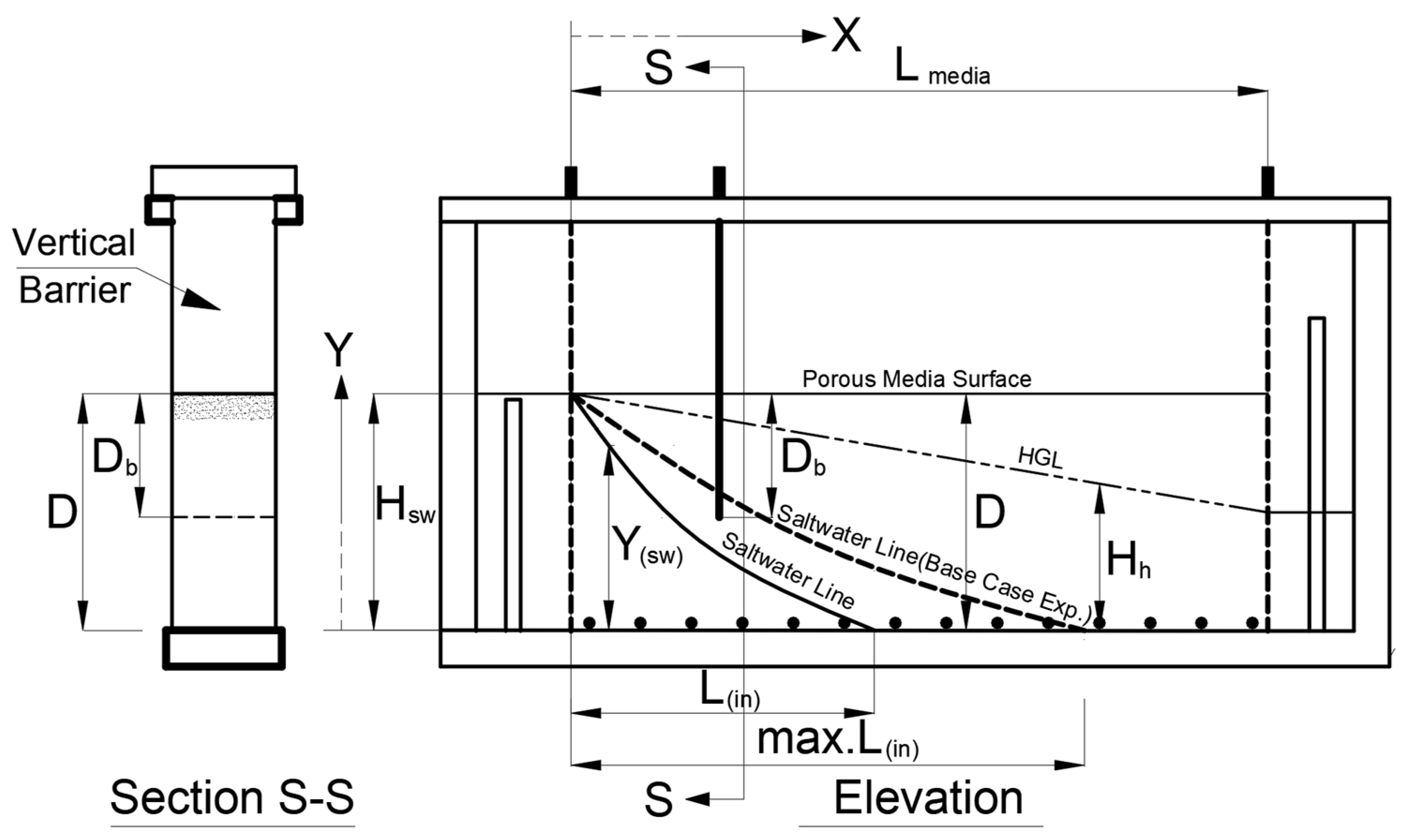
Two geometric parameters are used to assign the hydraulic gradient and saltwater profile.

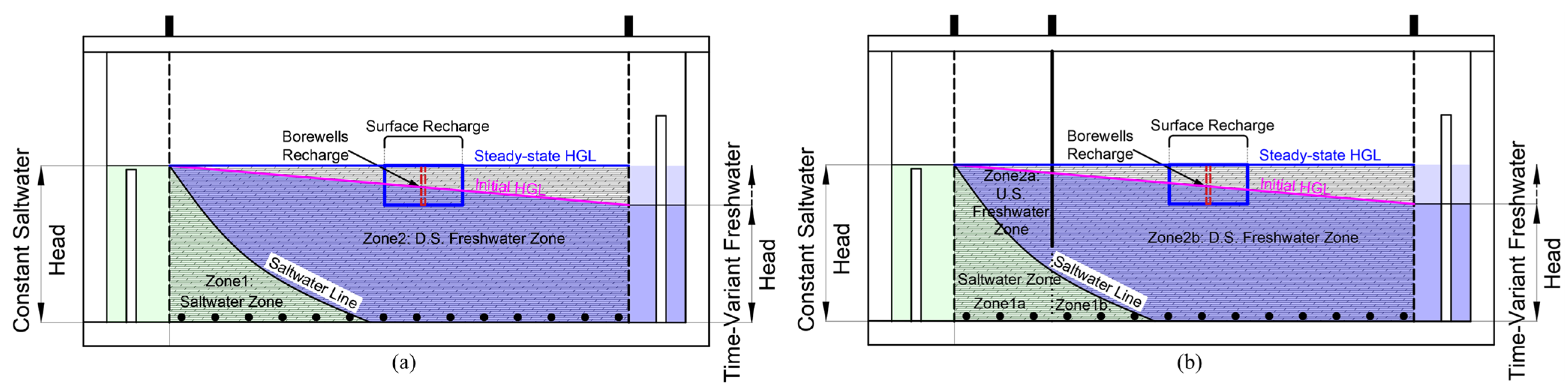
2.3. Conceptual Model

A proper conceptual model could be provided as a pre-set for developing a numerical model based on the experimental set and procedures previously presented in Section 2.1 and Section 2.2. The numerical investigation of saltwater intrusion will be conducted using either a traditional vertical barrier or artificial recharge approaches. To control seawater intrusion using a vertical barrier, various penetration depths will be simulated. Surface and subsurface recharge systems will be used as artificial recharge methods. To determine their effectiveness in controlling the saltwater intrusion problem, each of the management techniques is evaluated independently and in combination with vertical barrier.

Table 4. The studied cases using numerical simulation.

Category (a): Using Vertical Barrier
Model Cases	Description
Case1a	Base Case (Verification of experiment 1)
Case2a	BDR = 0.875
Case3a	BDR = 0.75 (Verification of experiment 2)
Case4a	BDR = 0.625
Case5a	BDR = 0.50
Case6a	BDR = 0.375
Case7a	BDR = 0.125
Category (b): using vertical barrier and surface recharge
Model Cases	Conditional Parameters
Case1b	Case1a + Surface Recharge
Case2b	Case2a + Surface Recharge
Case3b	Case3a + Surface Recharge
Case4b	Case4a + Surface Recharge
Case5b	Case5a + Surface Recharge
Case6b	Case6a + Surface Recharge
Case7b	Case7a + Surface Recharge
Category (c): using vertical barrier and subsurface recharge
Model Cases	Conditional Parameters
Case1c	Case1a + borewells Recharge
Case2c	Case2a + borewells Recharge
Case3c	Case3a + borewells Recharge
Case4c	Case4a + borewells Recharge
Case5c	Case5a + borewells Recharge
Case6c	Case6a + borewells Recharge
Case7c	Case7a + borewells Recharge

shows the numerical model cases being explored under different constraints. The suggested conceptual system is presented in Figure 6, taking into account the boundary heads, initial hydraulic grade line (HGL), barrier depth and location, and artificial recharge methods. When there is no vertical barrier, two water zones can be identified: zone 1 (saltwater zone) and zone 2 (freshwater zone), as shown in Figure 6a. After using a vertical barrier, zones 1 and 2 are further partitioned into two zones: zone 1a and zone 1b for saltwater and zone 2a and zone 2b for freshwater, as shown in Figure 6b. The key features of the conceptual system are outlined below.

• A constant-head saltwater boundary.
• A time-variant head freshwater boundary that advances from the initial head to equilibrium with the saltwater boundary in the steady-state condition.
• A vertical barrier of variable depths at a certain location.
• A source of surface and subsurface artificial recharge.

2.4. Numerical Model Development

MODFLOW-2005, in conjunction with the SWI2 package, through the ModelMuse software (version 4.3.0.0), is used in this study for numerical modeling of saltwater intrusion [58]. SWI2 is a ModelMuse software package used to analyze three-dimensional groundwater flow and model saltwater intrusion, and calculate hydraulic heads [59]. The main advantage of using the SWI2 package is that it requires fewer cells for the simulation process than variable-density groundwater flow packages like SEAWAT. The ability of SWI2 to represent each aquifer as a single layer of cells results in significant model run-time savings.

MODPATH is a ModelMuse post-processing package for particle tracking that computes and displays three-dimensional pathlines based on MODFLOW output [60]. The MODPATH packages are used to visualize the flow behavior of both freshwater and saltwater through the sand media by visualizing the expert transport trajectories coming from the saltwater boundary, the freshwater boundary, and the flow path from the recharge area for the cases defined in Table 4. The particle tracking in the MODPATH package is simulated in the forward tracking direction using cylinder particle placement, as illustrated in Figure 7b.

On the basis of the conceptual model, the saltwater boundary cells are represented by the General-Head Boundary (GHB) package. The Time-Variant Specified-Head (CHD) package is applied to the model freshwater boundary cells to obtain the same results as the experiments, with an initial hydraulic gradient of 0.085. The recharge value for each recharge type will be relevant to the flow across the saltwater boundary for each model case b, with the constraint that the hydraulic heads do not exceed the medium sand level as a maximum value. Various discretization systems are also examined in order to provide an accurate assessment of discrepancies in head drawdowns and water balances. In this study, 8 model layers with 2320 cell discretization are used, as shown in Figure 7a. Furthermore, as shown in Figure 7b, the flow direction will be characterized as +^veY, −^veY, +^veX, and −^veX.

2.4.1. Calibration and Verification Processes

Many factors contribute to groundwater model inconsistency, including hydrogeological properties, discretization, potential spatial discretization, time step, and solver parameters. Using the experimental results, many trials are carried out by the means of sensitivity analysis to calibrate the model using various hydrogeological properties, with reference to [61,62]. The transient stress period, on the other hand, will be assigned to be more than that needed for the experiment, with a proper equal interval time step. The impact of the heads on the cells and the accumulated volume water balance are evaluated. Following that, a verification procedure is implemented for:

• Confirming the time when a steady-state condition occurs based on the results of experiment 1.
• Fitting the observed saltwater line in experiments 1 and 2 for the transient and steady-state conditions.

2.4.2. Classification Ratios

As a starting point for selecting the best model case for controlling saltwater intrusion, four ratios are suggested to classify the model cases included in categories (a), (b), and (c). These ratios are calculated using the numerical results of the models. Each ratio is calculated for each model case and then classified by its value into best or worst. These ratios are the increase in saltwater ratio (SLR_i), repulsion ratio (R_r), wedge area ratio (WAR), and recharge ratio (RER). The four ratios are computed using the Equations (1)–(4), respectively, with the RER ratio computed only for cases in categories (b) and (c). The criteria for classifying the best model cases are that they have low values of SLR_i, WAR, and RER, as well as the maximum value of R_r. On the other hand, cases with high values of SLR_i, WAR, and RER, as well as the lowest value of R_r, are classified as the worst model cases and are not recommended for controlling saltwater intrusion. Because of the difficulty of having a model case have all the best or worst values of classification ratios to be classified as the best or worst model case (unclassified model case), it is important to use the DMM models to use the values of these classification ratios to make the final decision.

$${\mathrm{SLR}}_{\mathrm{i}}={\mathrm{SLR}}_{\mathrm{avg}}^{\mathrm{case}\mathrm{k}}-{\mathrm{SLR}}_{\mathrm{avg}}^{\mathrm{case}1\mathrm{a}}$$

(1)

$${\mathrm{R}}_{\mathrm{r}}={\mathrm{IR}}_{\mathrm{case}1\mathrm{a}}-{\mathrm{IR}}_{\mathrm{casek}}$$

(2)

$$\mathrm{WAR}=\frac{{\mathrm{Wedge}\mathrm{Area}}_{\mathrm{case}\left(\mathrm{k}\right)}}{{\mathrm{Wedge}\mathrm{Area}}_{\mathrm{case}1\mathrm{a}}}$$

(3)

$$\mathrm{RER}=\frac{{\mathrm{Recharge}}_{\mathrm{case}\left(\mathrm{j}\right)}}{{\mathrm{Saltwater}\mathrm{boundary}\mathrm{Recharge}}_{\mathrm{case}\left(\mathrm{j}\right)}}$$

(4)

where Wedge Area_case(k) is the wedge area for any case included at any category (a, b, and c), and Wedge Area_case(j) is the wedge area for the cases included at category (b) and category (c).

2.5. Decision-Making Model (AHP Technique)

The AHP technique is commonly employed in decision-making systems designed to aid in decision-making and rate options [63]. Actual metrics such as pricing, headcount, or subjective opinions are used as inputs into a numerical matrix in AHP. Ratio scales and consistency indices derived from eigenvalues and eigenvectors are among the results. The AHP model is a decision-making framework that assumes decision levels have a unidirectional hierarchical relationship [64]. AHP can study the interrelationships among all criteria using the hierarchical approach [65].

According to [66], there are three processes that go into creating AHP: model structure (decomposition), comparative judgment of alternatives and criteria, and priority synthesis. These methods can be broken down into four stages.

In the first stage, AHP divides a complex multi-criteria decision problem into a hierarchy of interrelated elements (criteria, decision alternatives). The criteria and alternatives are arranged in a family tree-like hierarchical structure. The next stage, after the problem has been decomposed and a hierarchy has been established, is to begin the comparison judgment process to evaluate the relative importance of the criteria within the grade. The criteria are compared pairwise at each grade based on their degrees of influence and the criteria provided at the higher grade. Pairwise comparisons are based on a nine-point scale, with 1 indicating “equal importance”, 3 indicating “slightly more important”, 5 indicating “much more important”, 7 indicating “highly more important”, and 9 indicating “extremely more important” [67,68]. These alternatives and criteria are evaluated based on the subjective opinions of experts represented by a point scale, including any intermediate value (2, 4, 6, and 8).

As demonstrated in Equation (5), the result of a pairwise comparison on n criteria can be summarized in a ${\left[\mathrm{X}\right]}_{\left(\mathrm{n}\ast \mathrm{n}\right)}$ evaluation matrix.

$$\begin{gathered} {\mathrm{C}}_1 {\mathrm{C}}_2\dots {\mathrm{C}}_{\mathrm{j}} \\ \left[\begin{array}{cccc}{\mathrm{x}}_{11}& {\mathrm{x}}_{12}& \cdots & {\mathrm{x}}_{1\mathrm{j}}\\ {\mathrm{x}}_{21}& {\mathrm{x}}_{22}& \cdots & {\mathrm{x}}_{2\mathrm{j}}\\ ⋮& ⋮& \ddots & ⋮\\ {\mathrm{x}}_{\mathrm{i}1}& {\mathrm{x}}_{\mathrm{j}2}& \cdots & {\mathrm{x}}_{\mathrm{ij}}\end{array}\right]\begin{array}{c}{C}_1\\ C_2\\ C_i\end{array} \end{gathered}$$

(5)

where: ${\mathrm{c}}_{\mathrm{j}}$ = 1, 2, 3… n—the set of criteria; ${\mathrm{x}}_{\mathrm{ij}}$ (ij = 1, 2, 3… n)—the weight quotient of the criteria; ${\mathrm{x}}_{\mathrm{ij}}$ = 1; ${\mathrm{x}}_{\mathrm{ji}}$= 1/${\mathrm{x}}_{\mathrm{ij}}$; ${\mathrm{x}}_{\mathrm{ij}}$≠ 0

The third stage, which comes after the dual comparison matrices, is to calculate the eigenvector, which shows the importance of each element in the relevant matrix with respect to the others [66].

In Equations (6) and (7), the % importance distribution of criteria is computed as follows:

$${\mathrm{b}}_{\mathrm{ij}}=\frac{{\mathrm{x}}_{\mathrm{ij}}}{{{\displaystyle \sum }}_{\mathrm{i}=1}^{\mathrm{n}}{\mathrm{x}}_{\mathrm{ij}}}$$

(6)

$${\mathrm{w}}_{\mathrm{i}}=\frac{{{\displaystyle \sum }}_{\mathrm{j}=1}^{\mathrm{n}}{\mathrm{b}}_{\mathrm{ij}}}{\mathrm{n}}$$

(7)

where: ${\mathrm{b}}_{\mathrm{ij}}$ the values of the normalized matrices; $\left[{\mathrm{w}}_{\mathrm{i}}\right]{}_{\mathrm{n}\ast 1}$ the percentage importance distribution of criteria; n—the number of criteria.

The fourth step is to ensure that the consistency ratio (CR) for each comparison matrix does not exceed 10% at the most.

A CR greater than 10% indicates inconsistency in the decision-maker’s judgments. The judgments in this case should be improved. Equations (8) and (9) are used to compute the CR value:

$${\left[{\mathrm{D}}_{\mathrm{i}}\right]}_{\mathrm{n}\ast 1}={\left[{\mathrm{x}}_{\mathrm{ij}}\right]}_{\mathrm{n}\ast \mathrm{n}}\times {\left[{\mathrm{w}}_{\mathrm{i}}\right]}_{\mathrm{n}\ast 1}$$

(8)

$${\mathsf{\lambda }}_{\max }=\frac{{{\displaystyle \sum }}_{\mathrm{i}=1}^{\mathrm{n}}\frac{{\mathrm{d}}_{\mathrm{i}}}{{\mathrm{w}}_{\mathrm{i}}}}{\mathrm{n}}$$

(9)

where: ${\mathsf{\lambda }}_{\max }$ is the matrix’s largest eigenvector and ${\left[D_i\right]}_{n\ast 1}$ is the weighted matrix.

Random Index (RI) is another value required to calculate CR. Provided by [69], the data include the RI values, which are constant numbers determined by the N value. Equation (10) specifies the calculation of the CR value based on this information.

$$\mathrm{CR}=\frac{{\mathsf{\lambda }}_{\max }-\mathrm{n}}{\left(\mathrm{n}-1\right)\times \mathrm{RI}}$$

(10)

where CR is the consistency ratio, ${\mathsf{\lambda }}_{\max }$ is the matrix’s largest eigenvector, RI is the random index, and n is the number of criteria.

In this study, it is suggested that an AHP-based model be used on two levels to find the best model case by comparing these model cases with the help of many ratios as a selection criterion. Through the AHP analysis, the model cases will be named as alternatives. The three alternatives (cases1a, 1b, and 1c) with no vertical barrier countermeasure will be eliminated from the total number of alternatives (21 alternatives), reducing the total number of alternatives to 18 alternatives (6 cases in each category). Level (1) involves the model dealing with three categories (a, b, and c) in order to select the best alternative from each. There are four criteria in category (a) (R_r, SLR_i, Minimum HHR, and WAR), and five in categories (b) and (c), with RER which is indicating the artificial recharge, and is exclusively utilized in categories (b) and (c). The top three alternatives from each of the three categories that emerged from level (1) can be used to create the final choice for the best alternative at level (2). Pairwise comparisons with other criteria aid in determining the relative importance of each criterion in the hierarchical structuring of the problem. The model’s first level consists of one matrix (4 × 4) for category (a) alternatives and one matrix (5 × 5) for categories (b) and (c) alternatives, reflecting the relative weights of the criteria as outputs. Moreover, five matrices (6 × 6) show the relative weight among the alternatives in the case of each criterion. The model, on the other hand, takes the same matrix for criteria weights and five matrices, each of which is (3 × 3), and expresses the relative weight among the final three alternatives for each criterion in its second level.

3. Results and Discussion

3.1. Senstivity Analysis, Calibration and Verification of the Numerical Model

The steady-state condition in experiment 1 (the base case) occurs 90 min after the experiment begins. To calibrate the numerical model, sensitivity analysis is implemented for the hydrogeological parameters, which include hydraulic conductivities in X, Y, and Z directions (k_x, k_y, k_z), specific yield (S_y), specific storage (S_s), and effective porosity (ŋ), as illustrated in Figure 8. Figure 8b,c demonstrate that the effect of both k_y and k_z on the intrusion length and average salt line elevation is negligible. Conversely, k_x, S_y, and S_s exhibit a directly proportional effect on the saltwater intrusion; however, they have a negligible impact on the average salt line elevation. In contrast, ŋ has an inversely proportional effect on both the saltwater intrusion and the average salt line elevation, with its influence becoming negligible after a ŋ value of 0.08. Considering the observed value of the saltwater line from experiment 1, the recommended values of the hydrogeological parameters are displayed in Figure 8. Subsequent trials led to

Table 5. Calibrated values of hydrogeological properties.

Hydrogeological Properties	kx (cm/s)	ky (cm/s)	kz (cm/s)	Sy	Ss	ŋ
Values	0.0069	0.0069	0.03	0.04	0.0619	0.0428

, which outlines the calibrated hydrogeological properties of the validated numerical model. The upcoming analysis will focus on the results at 90 min, considered as the steady-state condition.

As a validation of the numerical model steady-state simulation, Figure 9 shows the observed and simulated saltwater lines for various simulation times greater than 90 min. The figure shows that the simulated saltwater line closely matches the observed one, with RMSE values ranging from 0.90 to 1.19 for time ranging from 90 to 120 min, which confirms the occurrence of a steady-state condition after 90 min.

For transient results, the saltwater line for experiments 1 and 2 for simulation times of 30, 60, and 90 min is used to verify the corresponding results of the numerical model, as shown in Figure 10 and Figure 11. Both figures show that the model produces reasonable simulated results for the saltwater lines (case3a) when compared to the observed ones.

3.2. Behavior Evaluation of Saltwater Intrusion, Flow, and Hydraulic Heads for Categories (a), (b), and (c) Model Cases

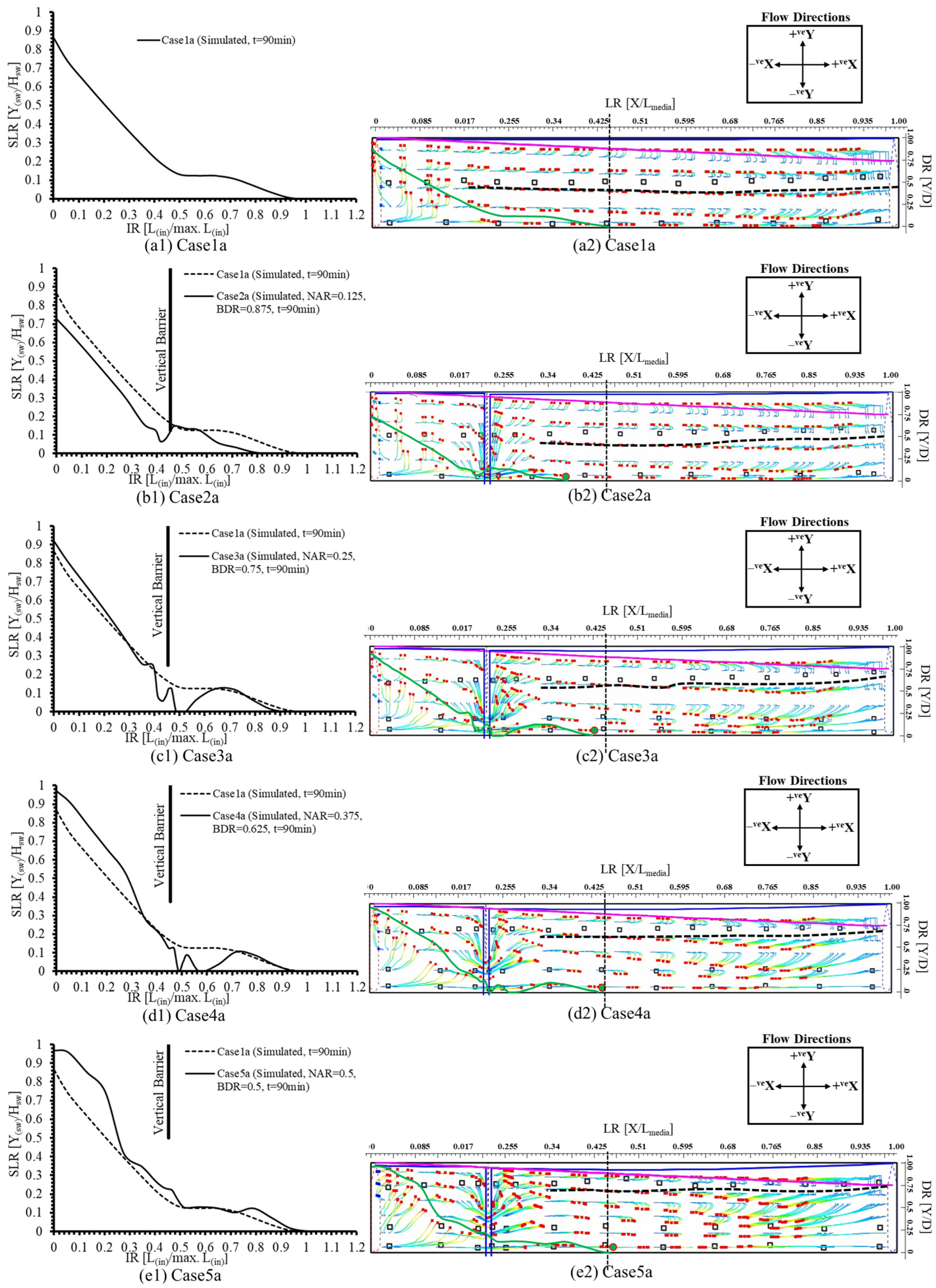
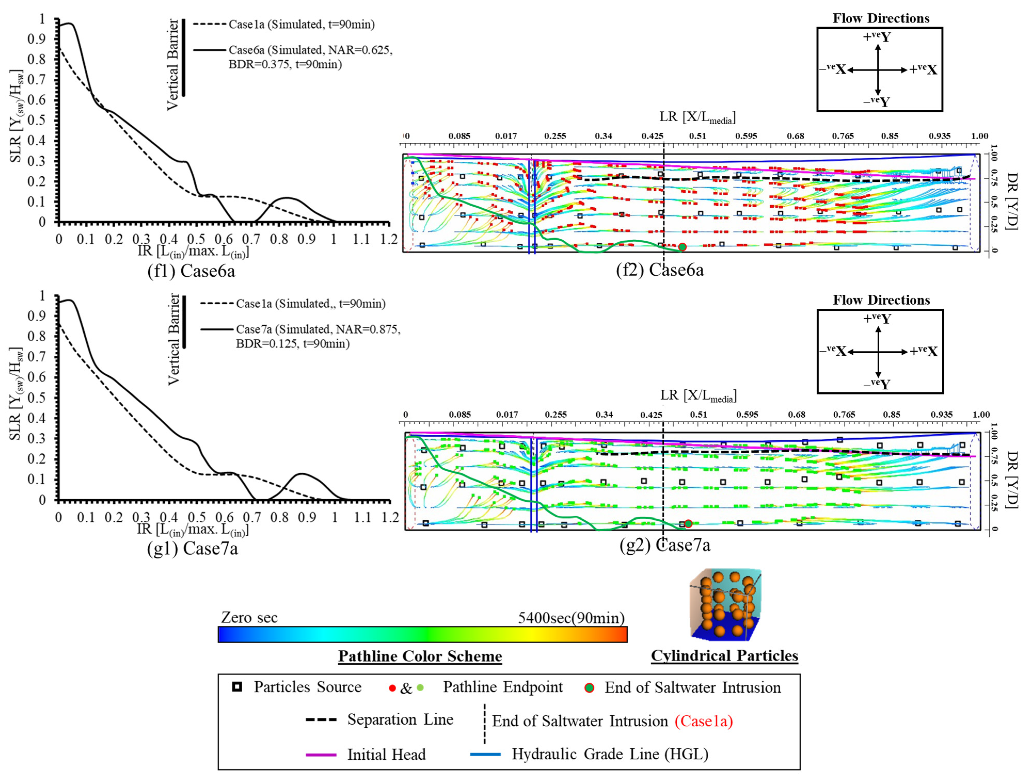
3.2.1. Saltwater Intrusion and Flow Behaviors in Category (a) Model Cases

The modeling results of saltwater intrusion and the accompanying flow behavior for the cases in category (a) will be discussed in this section. Two evaluation ratios are considered, including IR and the SLR_avg. Moreover, conditional parameters (BDR) and geometrical parameters (LR and DR) will be considered through the discussion. Figure 12 depicts these outcomes, and

Table 6. Values of the evaluation ratios and DR values for category (a) model cases.

Cases	Conditional Parameters	Evaluation Ratios		Geometrical Parameters
	BDR	IR	SLRavg	LRIntrusion	DRseparation
Case1a	---	0.97	0.28	0.45	0.37–0.45
Case2a	0.875	0.83	0.20	0.39	0.40–0.50
Case3a	0.75	0.90	0.23	0.42	0.50–0.68
Case4a	0.625	0.97	0.25	0.45	0.60–0.70
Case5a	0.50	0.97	0.31	0.45	0.69–0.75
Case6a	0.375	1.05	0.29	0.48	0.71–0.78
Case7a	0.125	1.05	0.32	0.48	0.76–0.85

provides a summary of the results.

Figures from Figure 12(a1–g1) as well as Table 6. reveal that case2a, which uses a vertical barrier with high BDR values, has the lowest evaluation ratio values (see Figure 12(b1)). Case7a’s evaluation ratios, on the other hand, have the highest values when a vertical barrier with low BDR values is applied (see Figure 12(g1)). Given these findings, flow behavior through the media sand needs to be investigated as an explanation for the variation in evaluation ratios.

Figures from Figure 12(a2–g2) depict the flow behavior of freshwater and saltwater. Figure 12(a2) depicts the flow behavior of case1a, demonstrating that the flow in zone 1 takes two directional flows: +^veY and +^veX. The +^veY flow conserves hydraulic heads near the saltwater boundary at the media sand level. Furthermore, the +^veX flow forces freshwater above the saltwater line to flow in the same direction as the saltwater. Freshwater flow directions in zone 2 are −^veX and +^veY in the upper half of the zone and −^veX and −^veY in the lower half of the zone. Because of the +^veY and −^veY flows in zone 2, a separation line with a DR value in the range of 0.37 to 0.45 could be identified, as illustrated in Table 6. and shown in Figure 12(a2). Along zone 2, the +^veY flow direction conserves the hydraulic head. In the upcoming analysis, the DR value of the separation line will be termed DR_separation.

Figure 12(b2) shows that the vertical barrier impedes freshwater flows from zone 2a to zone 2b, creating overlaying pressure in zone 1a, resulting in a dramatic drop and rise in the saltwater line shortly before and after the vertical barrier. Moreover, as shown in Table 6, the value of DR_separation increases to be in the range of 0.40 to 0.50 when compared to case1a.

The flow of freshwater from zone 2a to zone 2b is boosted by continuing to decrease BDR values, producing fluctuations in the saltwater line. Because of this flow, the overlying pressure of freshwater on zone 1a is reduced, leading the SLR value in this zone to rise (see Figure 12(c2–g2)). Furthermore, these figures and Table 6 show that DR_separation values are increasing, indicating that the majority of the freshwater flow in zone 2b is in the −^veY flow direction, resulting in hydraulic head reduction through this zone.

Based on the given results, it is possible to conclude that case2a has the lowest evaluation ratio values among the other cases. Furthermore, large DR_separation values, such as case7a, limit the hydraulic heads, creating an excess increase in the evaluation ratios (see Figure 12(g1,g2). In addition, adopting a vertical barrier with a high BDR ratio could effectively manage the saltwater intrusion. Furthermore, management of saltwater intrusion will be considered in this study by managing the DR_separation as well as the hydraulic heads along zone 2b using groundwater artificial recharge in conjunction with the use of a vertical barrier.

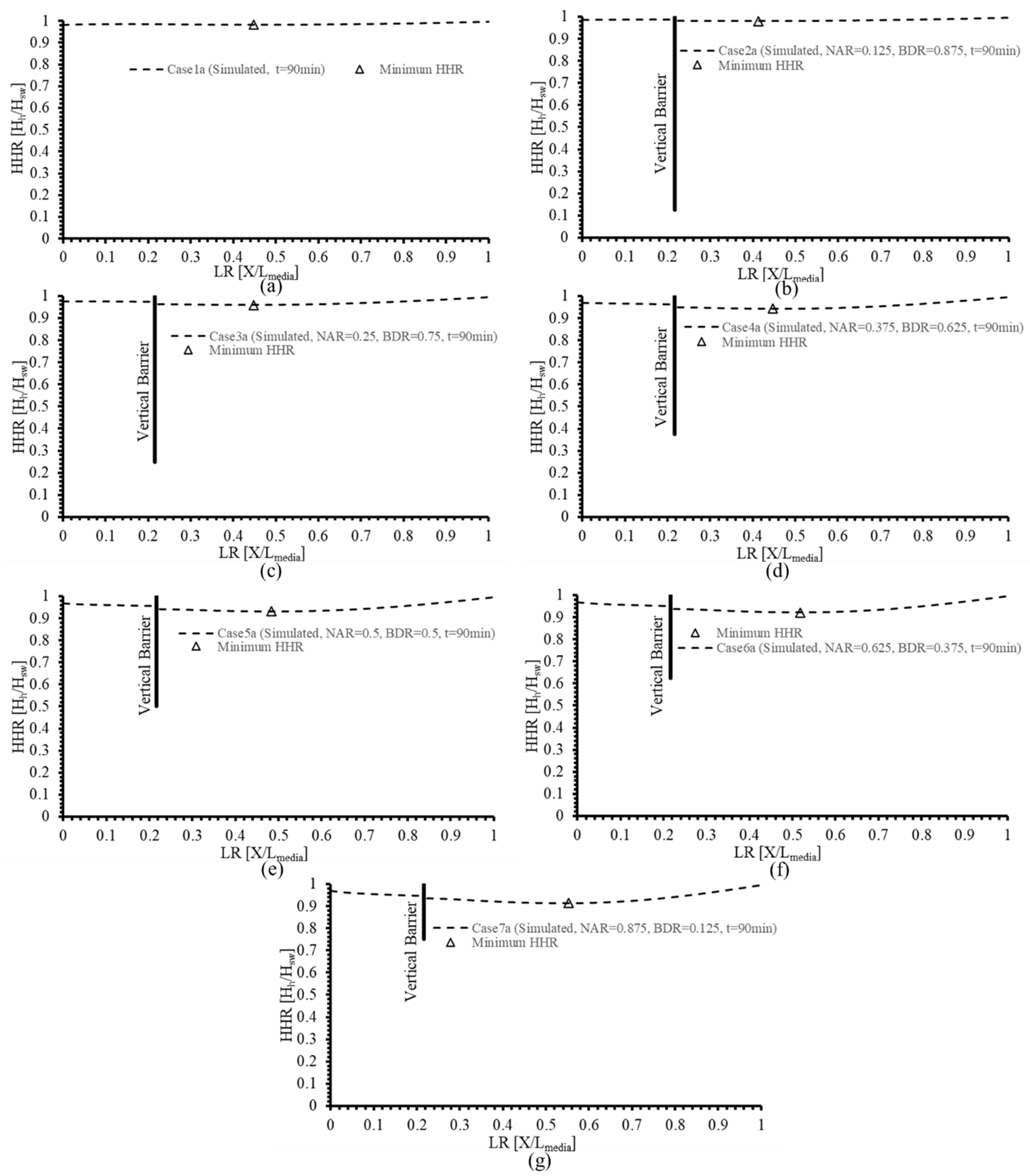
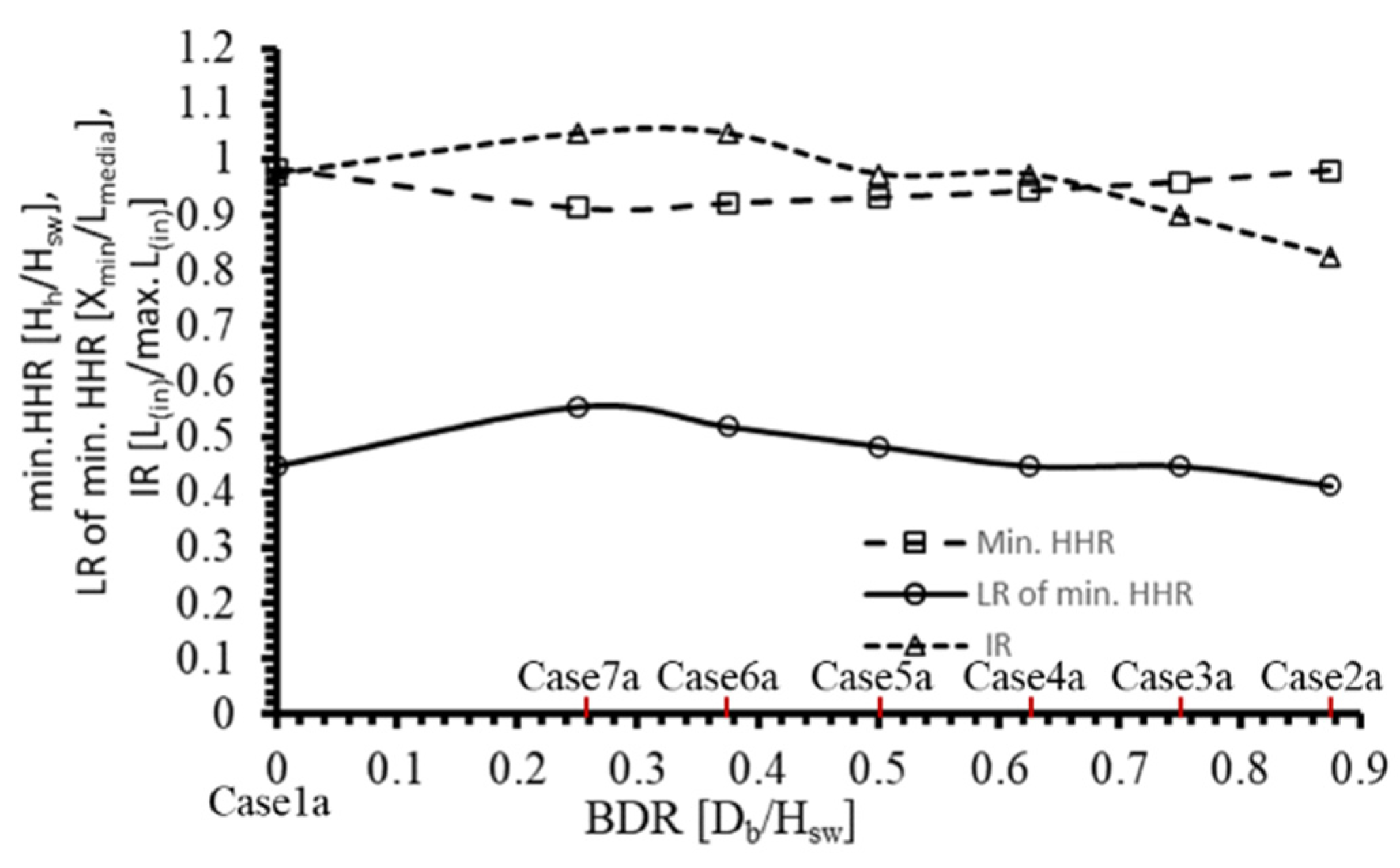
3.2.2. Hydraulic Head Variations in Category (a) Model Cases

As illustrated in Figure 13, the hydraulic head variations indicated by the HHR evaluation ratio are investigated for the category (a) model cases. This figure illustrates the relationship between HHR and LR ratios by displaying the minimum HHR values and their locations along the aquifer. Figure 13 shows that the hydraulic head of case7a has the lowest HHR value of 0.91 compared with the other cases (cases1a–6a) located at an LR value of 0.55 (see Figure 13g). On the other hand, case1a has the highest value of the minimum HHR (0.98), and its location has an LR of 0.44, as shown in Figure 13a.

The above results can be summarized as illustrated in Figure 14, which depicts the effect of BDR on the location (LR), the value of the minimum HHR, and the IR ratios. The minimum hydraulic head is located at zone 2b for all study cases (case1a–case7a), with LR values ranging from 0.45 to 0.55 and corresponding minimum HHR values ranging from 0.91 to 0.98. On the other hand, the maximum IR occurs for both cases6a and 7a with a value of 1.05 when using a BDR in the value range from 0.25 to 0.38. Given these findings, increasing the hydraulic head represented by HHR could effectively control saltwater intrusion when combined with the vertical barrier countermeasure. For this purpose, using groundwater artificial recharge, whether by surface or subsurface recharge, at the location of the minimum HHR value (LR in the range from 0.45 to 0.55), combined with the use of a vertical barrier, could be used to control saltwater intrusion, as will be discussed in the following sections of this study.

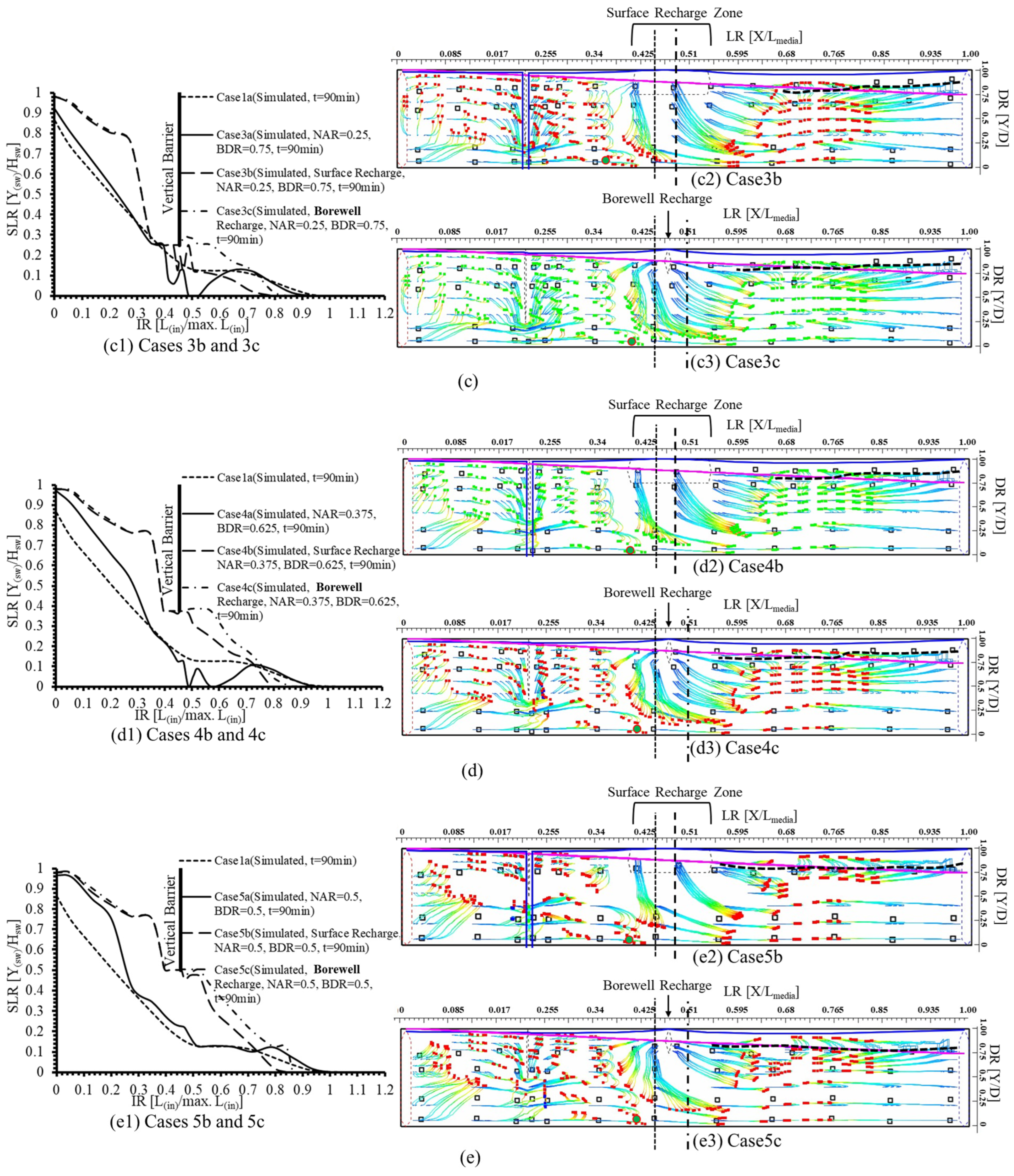
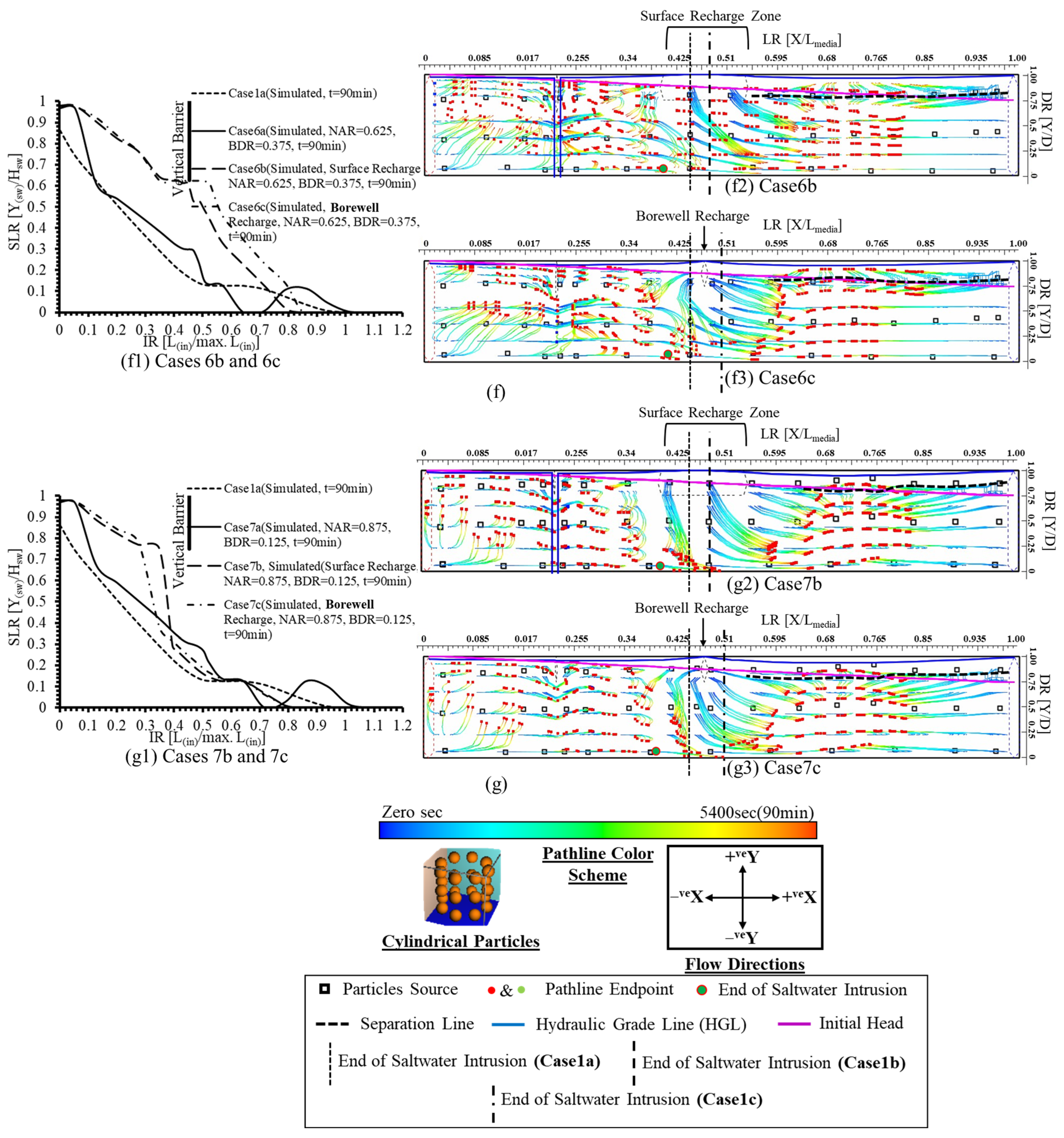
3.2.3. Saltwater Intrusion and Flow Behaviors in Categories (b) and (c) Model Cases

Groundwater artificial recharge is used to control saltwater intrusion in zone 2b along the LR range (from 0.45 to 0.55), which has a minimum value of HHR for preserving its value at the unity value. Surface and subsurface recharge are numerically discussed, either separately or in conjunction with the vertical barrier, as shown in Figure 15 for category (b) and category (c) model cases. The recharge is applied along the whole range of LR values from 0.45 to 0.55 for surface recharge. In contrast, for subsurface recharge, the recharge is applied as a line of wells at the midpoint of the same LR range at a value of 0.5. The results of category (b) and category (c) study cases will be compared with the base case results (case1a) and the corresponding cases of category (a) in the following discussions, as depicted in Figure 15 and summarized in

Table 7. Values of the evaluation ratios and DR values for categories (a), (b), and (c) model cases.

Category	Cases	Conditional Parameters	Evaluation Ratios		Geometrical Parameters
		BDR	IR	SLRavg	LRIntrusion	DRseparation
Category (a)	Case1a	---	0.97	0.28	0.45	0.37–0.45
	Case2a	0.875	0.83	0.20	0.39	0.40–0.50
	Case3a	0.75	0.90	0.23	0.42	0.50–0.68
	Case4a	0.625	0.97	0.25	0.45	0.60–0.70
	Case5a	0.50	0.97	0.31	0.45	0.69–0.75
	Case6a	0.375	1.05	0.29	0.48	0.71–0.78
	Case7a	0.125	1.05	0.32	0.48	0.76–0.85
Category (b)	Case1b	---	1.0	0.39	0.47	0.80–0.85
	Case2b	0.875	0.75	0.40	0.35	0.80–0.85
	Case3b	0.75	0.68	0.34	0.32	0.80–0.90
	Case4b	0.625	0.81	0.44	0.38	0.80–0.90
	Case5b	0.50	0.81	0.51	0.38	0.75–0.80
	Case6b	0.375	0.81	0.54	0.38	0.75–0.80
	Case7b	0.125	0.81	0.37	0.38	0.80–0.90
Category (c)	Case1c	---	1.05	0.41	0.49	0.80–0.85
	Case2c	0.875	0.82	0.35	0.38	0.80–0.85
	Case3c	0.75	0.82	0.38	0.38	0.80–0.90
	Case4c	0.625	0.85	0.45	0.40	0.80–0.90
	Case5c	0.50	0.85	0.52	0.40	0.75–0.80
	Case6c	0.375	0.85	0.57	0.40	0.75–0.80
	Case7c	0.125	0.75	0.39	0.40	0.80–0.90

.

As an analysis of the saltwater intrusion based on the evaluation ratios from Figure 15(a1–g1) as well as Table 7, it is found that case3b has the lowest IR value among all the model cases included in categories (a), (b), and (c). However, the SLR_avg values of case2a and case3b are the lowest, with case2a having a lower value than case3b.

The saltwater and freshwater flow behaviors could be described from Figure 15(a2–g2). In case1b, the surface recharge works as a hydraulic barrier that prevents saltwater from flowing in the +^veX direction as well as forcing it to flow intensively in the +^veY direction. This behavior causes an increase in the SLR_avg, compared with that of case1a, and the majority of recharged freshwater is forced to take a +^veX direction (see Figure 15(a2)). The flow behavior in case1c is similar to that in case1b (see Figure 15(a3)), but its SLR_avg is higher, indicating that the countermeasure effect of subsurface recharging, which is a line of wells, is less than that of surface recharge, which is a water mass.

In contrast to case2b, the value of SLR rises due to the −^veX flow direction of surface recharge toward the neck area beneath the vertical barrier, preventing the saltwater line from intruding (Figure 15(b2)). Because well recharge has a lower effect than surface recharge, the IR and LR ratios are higher in case2c than in case2b, as shown in Figure 15(b2,b3) and illustrated in Table 7.

In the case3b flow behavior, freshwater flows intensively from zone 2a to zone 2b (see Figure 15(c2)), causing SLR_avg to decline to become the least among the category (b) model cases. Because of the poor influence of well recharge, the SLR_avg value for case3c is greater than that of case3b, as demonstrated in Table 7. By continuing to lower BDR for cases4b, 5b, 6b, and 7b, as well as the corresponding cases in category (c), the freshwater flows from zone 2a to zone 2b in the +^veX direction, which reduces the effect of surface and well recharge, as shown in Table 7.

Because of the artificial recharge that applies in categories (b) and (c), the hydraulic heads along the experimental section are unchanged for all model cases, and the DR_separation is nearly the same with a value range from 0.75 to 0.90.

Based on the findings, it is possible to conclude that artificial aquifer recharging along the LR values from 0.45 to 0.55; which has a minimum value of the HHR ratio to conserve its value, as well as the unity accompanied by using a vertical barrier; has a significant effect on controlling saltwater intrusion. Furthermore, because of its body mass, surface recharge is more efficient than well recharge. Conclusively, the value of IR, as an evaluation ratio, for case3b is the lowest among all the cases included in categories (a), (b), and (c). However, the minimum value of SLR_avg is achieved in case2a, confirming the efficient combination of the vertical barrier and surface recharge at the location of the minimum HHR (LR in the range from 0.45 to 0.55).

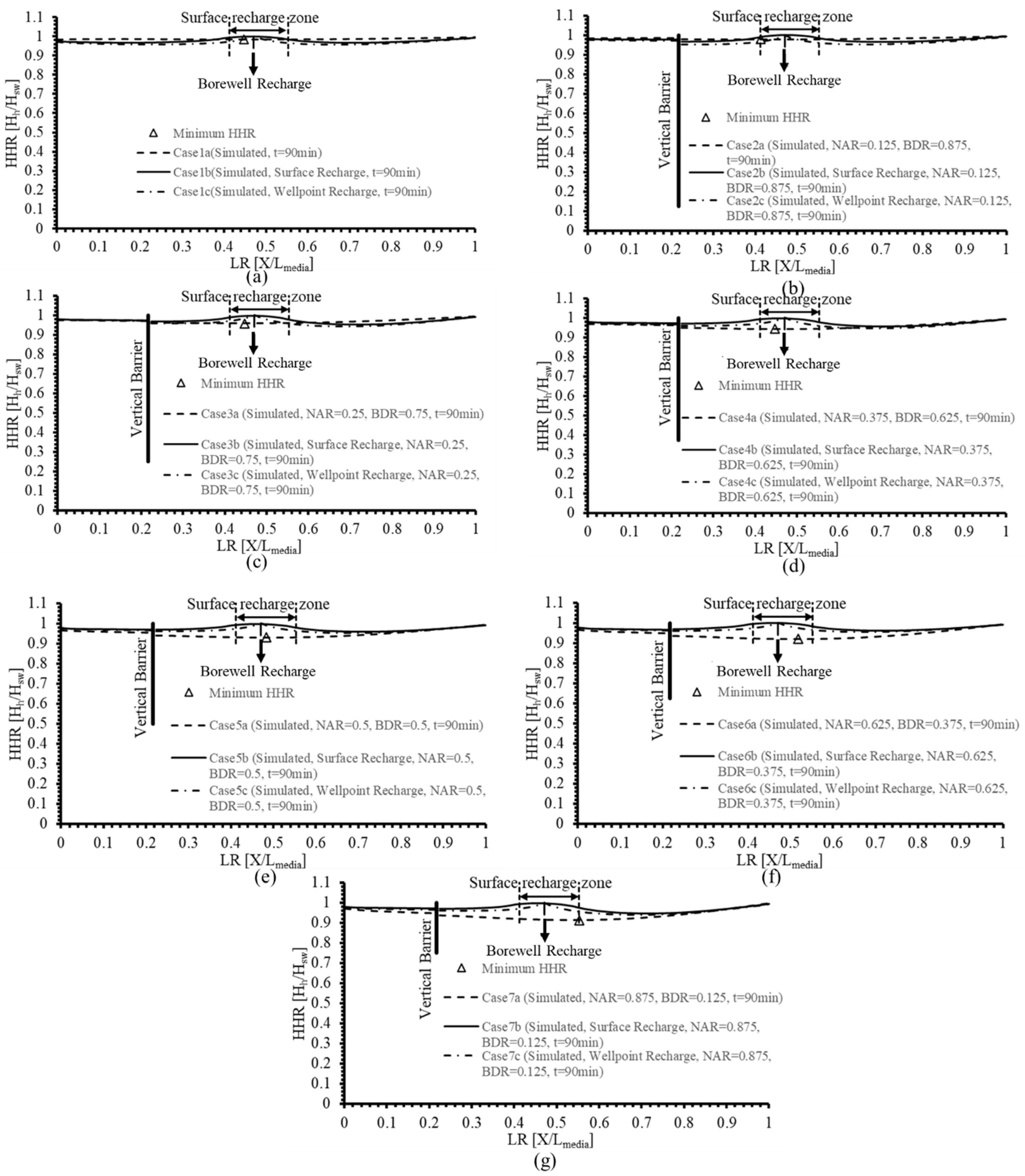
3.2.4. Hydraulic Head Variations in Categories (b) and (c) Model Cases

Figure 16a–g depict the hydraulic heads along the aquifer as represented by the HHR ratio for cases in categories (b) and (c) compared to category (a). The hydraulic heads for all cases have been conserved along the LR ratio from 0.45 to 0.55, which has the minimum value of HHR to have the unity value, and the losses through the vertical barrier are greatly reduced when compared to those of category (a).

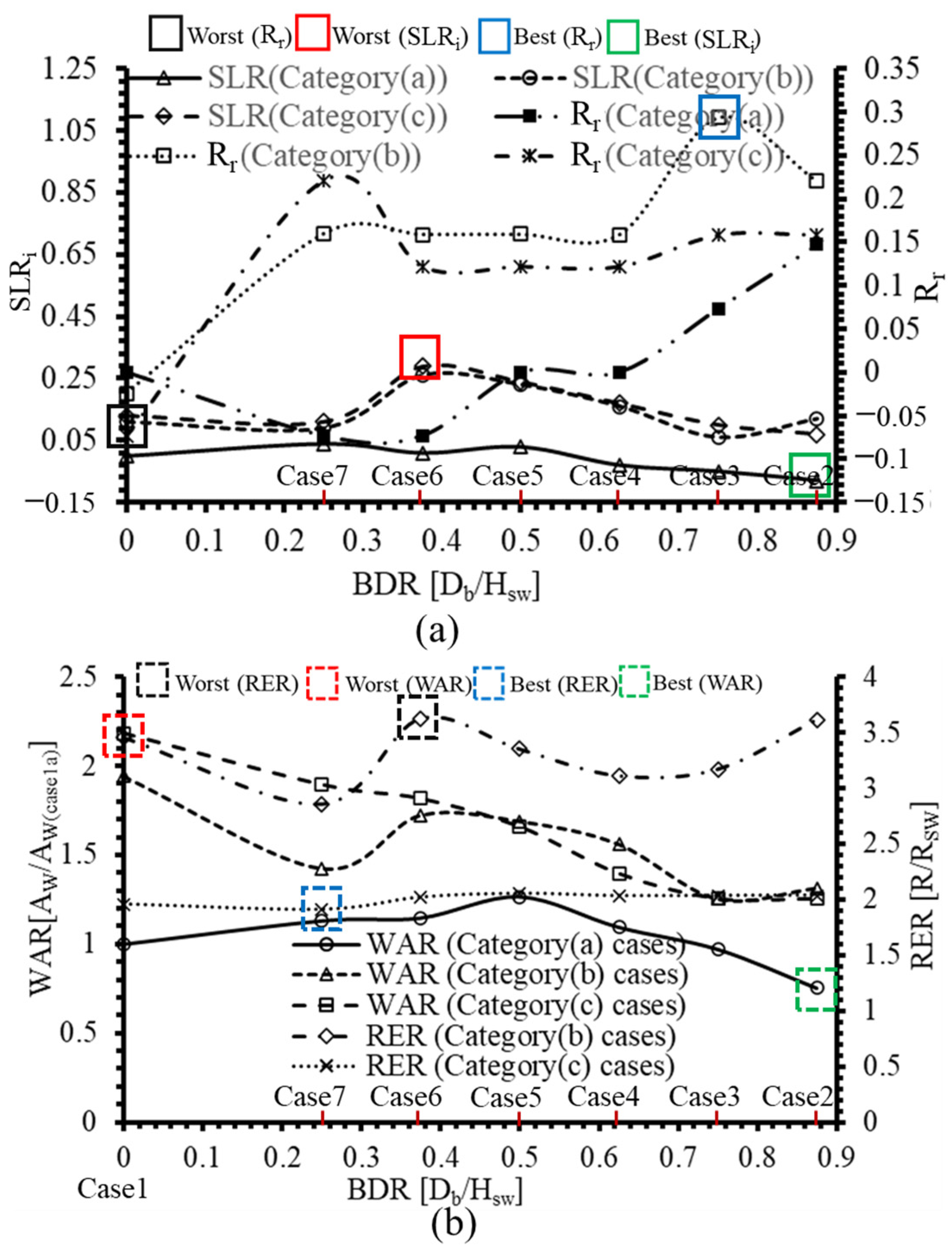
3.3. Classification of Model Cases

The classification ratios described in Section 2.4.2, Classification Ratios, are summarized and classified in Figure 17 and

Table 8. Model cases classification according to values of classification ratios.

Classification Ratio	Best	Worst
SLRi	Case2a (−0.08)	Case6c (0.29)
Rr	Case3b (0.29)	Case1c (−0.07)
WAR	Case2a (0.76)	Case1c (2.18)
RER	Case7c (1.91)	Case6b (3.62)

. Figure 17a presents the SLR_avg and R_r values for each model case, whereas Figure 17b depicts the WAR and RER values. Figure 17 and Table 8 show that case3b has the best R_r value of 0.29. Case2a, on the other hand, has the best SLR_avg and WAR values of −0.08 and 0.76, respectively. Furthermore, case7c has the best RER value of 1.91. On the contrary, case1c has the worst R_r and WAR values of −0.07 and 2.18, respectively. Furthermore, case6b has the worst RER value of 3.62. Moreover, case6c has the worst SLR_avg value of 3.62. The remaining model cases are categorized as unclassified model cases. Based on the findings, it is difficult to determine which model case is the most successful scenario to implement as a saltwater intrusion countermeasure. As a result, the DMM model is needed for determining the most effective model case.

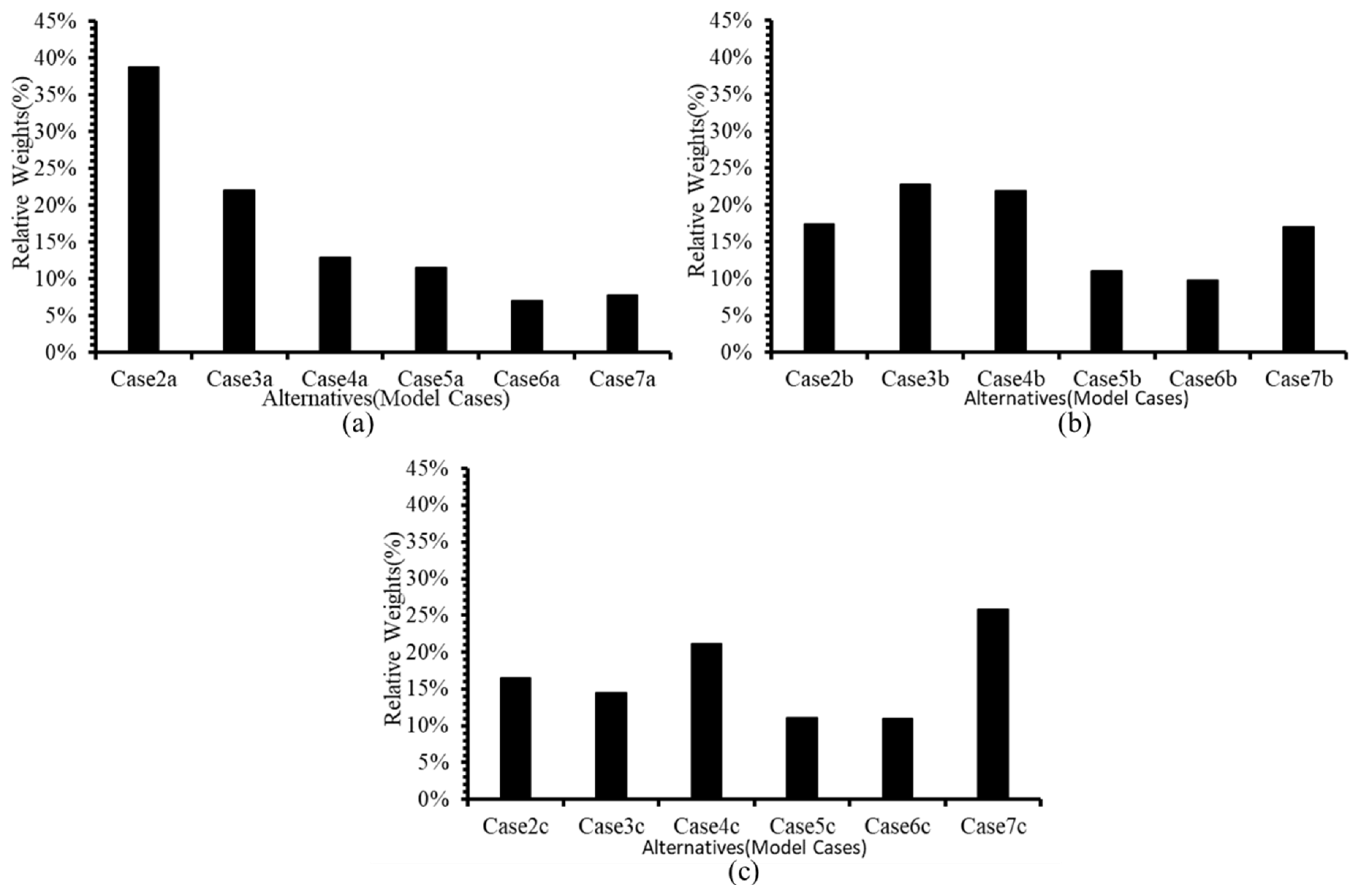
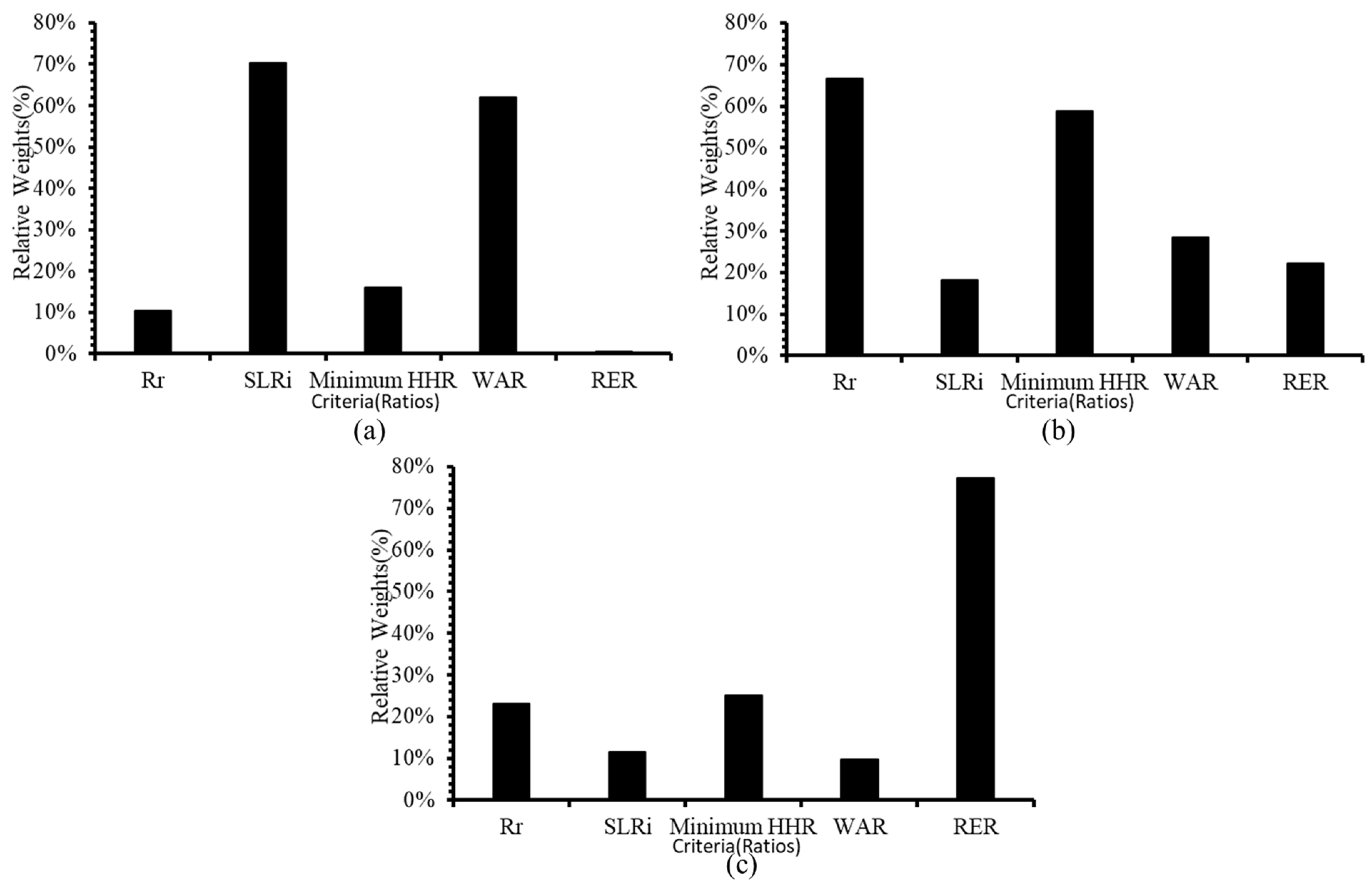
3.4. Selecting the Most Effective Model Case (AHP Application Results)

As previously stated, the AHP model is applied to the numerical model results at two different levels of selection (levels (1) and (2)). Model cases are referred to as alternatives at this stage, and selected ratios among the evaluation and classification ratios are referred to as criteria. Level (1) needs to determine the best alternative in each category. Furthermore, level (2) is for deciding the best alternative. For category (a) alternatives, the criteria values used include SLR_i, Minimum HHR, R_r, and WAR, and the RER is added over these ratios for categories (b) and (c).

3.4.1. Level (1) Results

For the alternatives in each category, the model is applied at level (1) using the weights chosen among criteria as shown in Figure 18. According to Figure 18a, minimum HHR has the largest weight for category (a) alternatives, followed by R_r. Also, WAR has the lowest weight. Similarly, for category (b) alternatives (see Figure 18b), the same rating is observed for minimum HHR (the highest weight), followed by R_r, while WAR has the lowest weight.

Figure 18 illustrates the results of the relative weights in the three categories for each alternative. It is clear that case2a ranks first in this category with a relative weight of 38.72%, then case3a, and case6a comes in last (see Figure 19a). Case3b is the best alternative in category (b), followed by case4b, which has a weight difference of 3.5% with case3b. Case6b is the worst alternative in this category (see Figure 19b). Case7c is the recommended alternative in category (c), with a weight of 25.83% ahead of the rest of the alternatives, followed by case4c, while case6c placed in last place in this category (see Figure 19c).

3.4.2. Level (2) Results

The model’s level (1) findings are summarized in the three best case model alternatives (cases2a, 3b, and 7c), as shown in Figure 19. Figure 20 summarizes the relative weights for each criterion in relation to the three alternatives. In case2a, SLR_i is the most effective criterion, followed by WAR, while RER has a negligible effect (Figure 20a). On the other hand, R_r is the most essential parameter influencing case3b, followed by minimum HHR (Figure 20b). Case7c is clearly influenced primarily by RER (Figure 20c).

As a result of the preceding findings, Figure 21 illustrates the weight values of the alternatives as a final decision, which clearly supports case3b by a percentage of 48% over a percentage of 27.30% for case7c and 25% for case2a. Based on the findings, it could be concluded that the components of case3b (combining the vertical barrier with surface recharge along the LR ratio from 0.45 to 0.55) could be classified as a best model case for use as a saltwater countermeasure. Furthermore, the vertical barrier has a greater effect when combined with surface recharge than when combined with well recharge. On the other hand, surface recharge necessitates a high recharge rate (about 1.25 times the borewell recharge).

4. Conclusions

In this study, saltwater intrusion is managed by controlling hydraulic heads along the coastal aquifer using surface or subsurface recharges in conjunction with the traditional vertical barrier countermeasure. A physical model is created to investigate the saltwater line behavior with a vertical barrier (experiment 1) and without a vertical barrier (experiment 2). The experimental results are used to validate a MODFLOW-created numerical model. Following that, three categories of model cases ((a), (b), and (c)), each with seven proposed model cases, are numerically investigated for: analyzing the saltwater–freshwater interaction through porous media; selecting the best location of the recharge; determining the best depth of the vertical barrier; and selecting the components of the efficient countermeasure system, including the vertical barrier, surface recharge, and subsurface recharge. Evaluation ratios are suggested in order to analyze and characterize the numerical model cases’ saltwater line and hydraulic head variations. According to category (a) simulation results, the minimum hydraulic head occurs through length ratio (LR) values ranging from 0.45 to 0.55, with corresponding values of hydraulic head ratio (HHR) ranging from 0.91 to 0.98. On the other hand, surface and subsurface recharge are implemented through categories (b) and (c) to investigate saltwater control by maintaining the HHR value of unity within the concluded LR range. As a pre-set for finding the best model case, classification ratios are proposed to classify the model cases included in the three mentioned categories as the best or worst model case. Using the calculated classification ratio values, an analytical hierarchy process (AHP) decision-making model (DMM) is used to select the best model case that is recommended for saltwater control using two selection levels. The first selection level concluded that the minimum HHR has the highest relative weight in all categories, while the WAR has the lowest. Cases2a, 3b, and 7c are rated as the best model cases in categories (a), (b), and (c), respectively, and are most affected by SLR_i, R_r, and RER, respectively. In the second selection level, the final decision is made that case3b is the overall best model case, which has a reasonable WAR of 1.25 and a maximum R_r of 0.29. The findings indicate that countermeasure systems (combining the vertical barrier with surface recharge) are the best choice to be used in similar cases. Furthermore, the suggested framework, which includes assigning the optimal recharge location and integrating the three models, could be examined in various geological formations and used in real-world cases.

While the numerical model is validated by RMSE and the problem is expressed in dimensionless form to reduce variables and facilitate application across different problem scales, it is crucial to consider potential future limitations and uncertainties. The use of an ideal homogeneous porous medium and a fixed vertical barrier location constrains the applicability of the study. Conversely, the parameters obtained during calibration are subject to inaccuracies resulting from the simplification of the complex experimental reality, and the presence of measurement noise introduces additional uncertainty. Therefore, the selected countermeasure components need to undergo testing in a real case with similar conditions, and the proposed framework should be applied to more intricate hydrogeological conditions in laboratory experiments or full-scale projects. Additionally, it is essential to investigate the optimal vertical barrier location in conjunction with recharging methods, as well as the implications of climate change, sea level fluctuations, and variations in water supply.

References

1. Abd-Elaty, I.; Abd-Elhamid, H.F.; Negm, A.M. Investigation of Saltwater Intrusion in Coastal Aquifers. In Groundwater in the Nile Delta; Negm, A.M., Ed.; Springer International Publishing: Cham, Switzerland, 2019; pp. 329–353. [Google Scholar] [CrossRef]
2. Sutar, A.; Rotte, V. Prevention of Saltwater Intrusion: A Laboratory-Scale Study on Electrokinetic Remediation; Springer: Singapore, 2022; pp. 389–400. [Google Scholar]
3. Qi, S.-Z.; Qiu, Q.-L. Environmental hazard from saltwater intrusion in the Laizhou Gulf, Shandong Province of China. Nat. Hazards 2011, 56, 563–566. [Google Scholar] [CrossRef]
4. Shi, L.; Jiao, J.J. Seawater intrusion and coastal aquifer management in China: A review. Environ. Earth Sci. 2014, 72, 2811–2819. [Google Scholar] [CrossRef]
5. Anders, R.; Mendez, G.O.; Futa, K.; Danskin, W.R. A Geochemical Approach to Determine Sources and Movement of Saline Groundwater in a Coastal Aquifer. Groundwater 2014, 52, 756–768. [Google Scholar] [CrossRef] [PubMed]
6. Cary, L.; Petelet-Giraud, E.; Bertrand, G.; Kloppmann, W.; Aquilina, L.; Martins, V.; Hirata, R.; Montenegro, S.; Pauwels, H.; Chatton, E.; et al. Origins and processes of groundwater salinization in the urban coastal aquifers of Recife (Pernambuco, Brazil): A multi-isotope approach. Sci. Total. Environ. 2015, 530–531, 411–429. Available online: https://www.sciencedirect.com/science/article/pii/S0048969715300723 (accessed on 1 September 2023). [CrossRef] [PubMed]
7. Gopinath, S.; Srinivasamoorthy, K. Application of Geophysical and Hydrogeochemical Tracers to Investigate Salinisation Sources in Nagapatinam and Karaikal Coastal Aquifers, South India. Aquat. Procedia 2015, 4, 65–71. [Google Scholar] [CrossRef]
8. Abd-Elhamid, H.F. Investigation and control of seawater intrusion in the Eastern Nile Delta aquifer considering climate change. Water Supply 2016, 17, 311–323. [Google Scholar] [CrossRef]
9. Eissa, M.A.; de Dreuzy, J.-R.; Parker, B. Integrative management of saltwater intrusion in poorly-constrained semi-arid coastal aquifer at Ras El-Hekma, Northwestern Coast, Egypt. Groundw. Sustain. Dev. 2018, 6, 57–70. Available online: https://www.sciencedirect.com/science/article/pii/S2352801X16300704 (accessed on 1 October 2023). [CrossRef]
10. Abd-Elhamid, H.F.; Abd-Elaty, I.; Negm, A.M. Control of Saltwater Intrusion in Coastal Aquifers. In Groundwater in the Nile Delta; Negm, A.M., Ed.; Springer International Publishing: Cham, Switzerland, 2019; pp. 355–384. [Google Scholar] [CrossRef]
11. Pramada, S.K.; Minnu, K.P.; Roshni, T. Insight into sea water intrusion due to pumping: A case study of Ernakulam coast, India. ISH J. Hydraul. Eng. 2021, 27, 442–451. [Google Scholar] [CrossRef]
12. Abd-Elhamid, H.F.; Javadi, A.A. A Cost-Effective Method to Control Seawater Intrusion in Coastal Aquifers. Water Resour. Manag. 2011, 25, 2755–2780. [Google Scholar] [CrossRef]
13. Kallioras, A.; Pliakas, F.-K.; Schüth, C.; Rausch, R. Methods to Countermeasure the Intrusion of Seawater into Coastal Aquifer Systems. In Wastewater Reuse and Management; Springer: Dordrecht, The Netherlands, 2013; pp. 470–490. [Google Scholar]
14. Cai, J.; Taute, T.; Schneider, M. Recommendations of Controlling Saltwater Intrusion in an Inland Aquifer for Drinking-Water Supply at a Certain Waterworks Site in Berlin (Germany). Water Resour. Manag. 2015, 29, 2221–2232. [Google Scholar] [CrossRef]
15. Huang, P.-S.; Chiu, Y.-C. A Simulation-Optimization Model for Seawater Intrusion Management at Pingtung Coastal Area, Taiwan. Water 2018, 10, 251. [Google Scholar] [CrossRef]
16. Hussain, M.S.; Abd-Elhamid, H.F.; Javadi, A.A.; Sherif, M.M. Management of Seawater Intrusion in Coastal Aquifers: A Review. Water 2019, 11, 2467. [Google Scholar] [CrossRef]
17. Raja Shekar, P.; Mathew, A. Assessing groundwater potential zones and artificial recharge sites in the monsoon-fed Murredu river basin, India: An integrated approach using GIS, AHP, and Fuzzy-AHP. Groundw. Sustain. Dev. 2023, 23, 100994. Available online: https://www.sciencedirect.com/science/article/pii/S2352801X23000942 (accessed on 1 October 2023). [CrossRef]
18. Shafa, N.S.; Babazadeh, H.; Aghayari, F.; Saremi, A. Optimal utilization of groundwater resources and artificial recharge system of Shahriar plain aquifer, Iran. Phys. Chem. Earth Parts A/B/C 2023, 129, 103358. Available online: https://www.sciencedirect.com/science/article/pii/S1474706523000025 (accessed on 1 October 2023). [CrossRef]
19. Wadi, D.; Wu, W.; Malik, I.; Fuad, A.; Thaw, M.M. Assessment and feasibility of the potential artificial groundwater recharge in semi-arid crystalline rocks context, Biteira district, Sudan. Sci. Afr. 2022, 17, e01298. Available online: https://www.sciencedirect.com/science/article/pii/S2468227622002058 (accessed on 1 September 2023). [CrossRef]
20. Ríos, I.H.; Cruz-Pérez, N.; Chirivella-Guerra, J.I.; García-Gil, A.; Rodríguez-Alcántara, J.S.; Rodríguez-Martín, J.; Marazuela, M.; Santamarta, J.C. Proposed recharge of island aquifer by deep wells with regenerated water in Gran Canaria (Spain). Groundw. Sustain. Dev. 2023, 22, 100959. Available online: https://www.sciencedirect.com/science/article/pii/S2352801X23000590 (accessed on 1 October 2023). [CrossRef]
21. Hasan, M.B.; Driessen, P.P.J.; Majumder, S.; Zoomers, A.; van Laerhoven, F. Factors Affecting Consumption of Water from a Newly Introduced Safe Drinking Water System: The Case of Managed Aquifer Recharge (MAR) Systems in Bangladesh. Water 2019, 11, 2459. [Google Scholar] [CrossRef]
22. Maliva, R.G. Surface-Spreading AAR Systems (Non-basin). In Anthropogenic Aquifer Recharge: WSP Methods in Water Resources Evaluation Series No 5; Springer International Publishing: Cham, Switzerland, 2020; pp. 517–565. [Google Scholar] [CrossRef]
23. Maliva, R.G. Surface Spreading System—Infiltration Basins. In Anthropogenic Aquifer Recharge: WSP Methods in Water Resources Evaluation Series No 5; Springer International Publishing: Cham, Switzerland, 2020; pp. 469–515. [Google Scholar] [CrossRef]
24. Environmental and Water Resources Institute (U.S.). Standard Guidelines for Artificial Recharge of Ground Water; American Society of Civil Engineers: Reston, VA, USA, 2001; Available online: https://ascelibrary.org/doi/book/10.1061/9780784405482 (accessed on 26 October 2023).
25. Maliva, R.G. ASR and Aquifer Recharge Using Wells. In Anthropogenic Aquifer Recharge: WSP Methods in Water Resources Evaluation Series No 5; Springer International Publishing: Cham, Switzerland, 2020; pp. 381–436. [Google Scholar] [CrossRef]
26. Robinson, G.; Ahmed, A.A.; Hamill, G. Experimental saltwater intrusion in coastal aquifers using automated image analysis: Applications to homogeneous aquifers. J. Hydrol. 2016, 538, 304–313. Available online: https://www.sciencedirect.com/science/article/pii/S0022169416301986 (accessed on 1 August 2023). [CrossRef]
27. Panthi, J.; Pradhanang, S.M.; Nolte, A.; Boving, T.B. Saltwater intrusion into coastal aquifers in the contiguous United States—A systematic review of investigation approaches and monitoring networks. Sci. Total. Environ. 2022, 836, 155641. Available online: https://www.sciencedirect.com/science/article/pii/S0048969722027371 (accessed on 1 September 2023). [CrossRef] [PubMed]
28. Mantoglou, A. Pumping management of coastal aquifers using analytical models of saltwater intrusion. Water Resour. Res. 2003, 39, 1335. Available online: https://agupubs.onlinelibrary.wiley.com/doi/abs/10.1029/2002WR001891 (accessed on 1 April 2023). [CrossRef]
29. Zhou, X.; Chen, M.; Liang, C. Optimal schemes of groundwater exploitation for prevention of seawater intrusion in the Leizhou Peninsula in southern China. Environ. Geol. 2003, 43, 978–985. [Google Scholar] [CrossRef]
30. Abarca, E.; Vázquez-Suñé, E.; Carrera, J.; Capino, B.; Gámez, D.; Batlle, F. Optimal design of measures to correct seawater intrusion. Water Resour. Res. 2006, 42, W09415. Available online: https://agupubs.onlinelibrary.wiley.com/doi/abs/10.1029/2005WR004524 (accessed on 1 September 2023). [CrossRef]
31. Sutherland, J.; Barfuss, S.L. Composite modelling: Combining physical and numerical models. In Proceedings of the 34th World Congress of the International Association for Hydro-Environment Engineering and Research (IAHR), Brisbane, Australia, 26 June–1 July 2011; pp. 4505–4512. [Google Scholar]
32. Singh, A. Managing the environmental problem of seawater intrusion in coastal aquifers through simulation–optimization modeling. Ecol. Indic. 2015, 48, 498–504. Available online: https://www.sciencedirect.com/science/article/pii/S1470160X14004191 (accessed on 1 October 2023). [CrossRef]
33. Guo, Q.; Huang, J.; Zhou, Z.; Wang, J. Experiment and Numerical Simulation of Seawater Intrusion under the Influences of Tidal Fluctuation and Groundwater Exploitation in Coastal Multilayered Aquifers. Geofluids 2019, 2019, 2316271. [Google Scholar] [CrossRef]
34. Armanuos, A.M.; Ibrahim, M.G.; Mahmod, W.E.; Takemura, J.; Yoshimura, C. Analysing the Combined Effect of Barrier Wall and Freshwater Injection Countermeasures on Controlling Saltwater Intrusion in Unconfined Coastal Aquifer Systems. Water Resour. Manag. 2019, 33, 1265–1280. [Google Scholar] [CrossRef]
35. Vaidya, O.S.; Kumar, S. Analytic hierarchy process: An overview of applications. Eur. J. Oper. Res. 2006, 169, 1–29. [Google Scholar] [CrossRef]
36. Alwetaishi, M.; Gadi, M.; Issa, U. Reliance of building energy in various climatic regions using multi criteria. Int. J. Sustain. Built Environ. 2017, 6, 555–564. [Google Scholar] [CrossRef]
37. Arunbose, S.; Srinivas, Y.; Rajkumar, S.; Nair, N.C.; Kaliraj, S. Remote sensing, GIS and AHP techniques based investigation of groundwater potential zones in the Karumeniyar river basin, Tamil Nadu, southern India. Groundw. Sustain. Dev. 2021, 14, 100586. [Google Scholar] [CrossRef]
38. Osiakwan, G.M.; Gibrilla, A.; Kabo-Bah, A.T.; Appiah-Adjei, E.K.; Anornu, G. Delineation of groundwater potential zones in the Central Region of Ghana using GIS and fuzzy analytic hierarchy process. Model. Earth Syst. Environ. 2022, 8, 5305–5326. [Google Scholar] [CrossRef]
39. Ahmadi, H.; Kaya, O.A.; Babadagi, E.; Savas, T.; Pekkan, E. GIS-Based Groundwater Potentiality Mapping Using AHP and FR Models in Central Antalya, Turkey. Environ. Sci. Proc. 2021, 5, 11. [Google Scholar]
40. Castillo, J.L.U.; Cruz, D.A.M.; Leal, J.A.R.; Vargas, J.T.; Tapia, S.A.R.; Celestino, A.E.M. Delineation of Groundwater Potential Zones (GWPZs) in a Semi-Arid Basin through Remote Sensing, GIS, and AHP Approaches. Water 2022, 14, 2138. [Google Scholar] [CrossRef]
41. Achu, A.L.; Thomas, J.; Reghunath, R. Multi-criteria decision analysis for delineation of groundwater potential zones in a tropical river basin using remote sensing, GIS and analytical hierarchy process (AHP). Groundw. Sustain. Dev. 2020, 10, 100365. [Google Scholar] [CrossRef]
42. Kumar, P.J.S.; Elango, L.; Schneider, M. GIS and AHP Based Groundwater Potential Zones Delineation in Chennai River Basin (CRB), India. Sustainability 2022, 14, 1830. [Google Scholar] [CrossRef]
43. Nithya, C.N.; Srinivas, Y.; Magesh, N.; Kaliraj, S. Assessment of groundwater potential zones in Chittar basin, Southern India using GIS based AHP technique. Remote. Sens. Appl. Soc. Environ. 2019, 15, 100248. [Google Scholar] [CrossRef]
44. Zghibi, A.; Mirchi, A.; Msaddek, M.H.; Merzougui, A.; Zouhri, L.; Taupin, J.-D.; Chekirbane, A.; Chenini, I.; Tarhouni, J. Using Analytical Hierarchy Process and Multi-Influencing Factors to Map Groundwater Recharge Zones in a Semi-Arid Mediterranean Coastal Aquifer. Water 2020, 12, 2525. [Google Scholar] [CrossRef]
45. Phin, T.T.; Hoa, D.T.B.; Trong, T.D.; Hai, D.T.; Que, P.T.N. Mapping vulnerability water supply in Rach Gia city due to saline intrusion on using analytical hierarchy process. Sustain. Water Resour. Manag. 2022, 8, 137. [Google Scholar] [CrossRef]
46. Mallick, J.; Khan, R.A.; Ahmed, M.; Alqadhi, S.D.; Alsubih, M.; Falqi, I.; Hasan, M.A. Modeling Groundwater Potential Zone in a Semi-Arid Region of Aseer Using Fuzzy-AHP and Geoinformation Techniques. Water 2019, 11, 2656. [Google Scholar] [CrossRef]
47. Shao, Z.; Huq, E.; Cai, B.; Altan, O.; Li, Y. Integrated remote sensing and GIS approach using Fuzzy-AHP to delineate and identify groundwater potential zones in semi-arid Shanxi Province, China. Environ. Model. Softw. 2020, 134, 104868. [Google Scholar] [CrossRef]
48. Gangadharan, R.; Nila Rekha, P.; Vinoth, S. Assessment of groundwater vulnerability mapping using AHP method in coastal watershed of shrimp farming area. Arab. J. Geosci. 2016, 9, 107. [Google Scholar] [CrossRef]
49. Güllü, Ö.; Kavurmacı, M. Investigation of temporal variation of groundwater salinity potential using AHP-based index. Environ. Monit. Assess. 2023, 195, 365. [Google Scholar] [CrossRef]
50. Yang, H.; Jia, C.; Li, X.; Yang, F.; Wang, C.; Yang, X. Evaluation of seawater intrusion and water quality prediction in Dagu River of North China based on fuzzy analytic hierarchy process exponential smoothing method. Environ. Sci. Pollut. Res. 2022, 29, 66160–66176. [Google Scholar] [CrossRef] [PubMed]
51. Pham, Q.N.; Ta, T.T.; Le Tran, T.; Pham, T.T.; Nguyen, T.C. Assessment of Saltwater Intrusion Vulnerability in the Coastal Aquifers in Ninh Thuan, Vietnam BT—Global Changes and Sustainable Development in Asian Emerging Market Economies. In Proceedings of EDESUS 2019; Nguyen, A.T., Hens, L., Eds.; Springer International Publishing: Cham, Switzerland, 2022; Volume 2, pp. 703–712. [Google Scholar]
52. Yokochi, R.; Zappala, J.C.; Purtschert, R.; Mueller, P. Origin of water masses in Floridan Aquifer System revealed by 81Kr. Earth Planet. Sci. Lett. 2021, 569, 117060. Available online: https://www.sciencedirect.com/science/article/pii/S0012821X21003150 (accessed on 1 October 2023). [CrossRef]
53. Halley, R.B.; Vacher, H.L.; Shinn, E.A. Geology and hydrogeology of the Florida Keys. In Geology and Hydrogeology of Carbonate Islands; Elsevier: Amsterdam, The Netherlands, 1997; pp. 217–248. Available online: https://pubs.usgs.gov/publication/70128983 (accessed on 26 October 2023).
54. Faye, S.; Faye, S.C.; Ndoye, S.; Faye, A. Hydrogeochemistry of the Saloum (Senegal) superficial coastal aquifer. Environ. Geol. 2003, 44, 127–136. [Google Scholar] [CrossRef]
55. Willis, S.S.; Johannesson, K.H. Controls on the geochemistry of rare earth elements in sediments and groundwaters of the Aquia aquifer, Maryland, USA. Chem. Geol. 2011, 285, 32–49. Available online: https://www.sciencedirect.com/science/article/pii/S0009254111000970 (accessed on 26 October 2023). [CrossRef]
56. Iashvili, T. HYDrogeological Conditions in Urban Areas in the Georgian Black Sea Coastal Zone Bt—Urban Groundwater Management and Sustainability; Tellam, J.H., Rivett, M.O., Israfilov, R.G., Herringshaw, L.G., Eds.; Springer: Dordrecht, The Netherlands, 2006; pp. 441–446. [Google Scholar]
57. G.U.N.T. G.U.N.T [Internet]. Equipment for Engineering Education. Available online: https://www.gunt.de/en/products/hydraulics-for-civil-engineering/hydraulic-engineering/seepage-flow/visualisation-of-seepage-flows/070.16900/hm169/glct-1:pa-148:ca-181:pr-768 (accessed on 14 September 2023).
58. Harbaugh, A.W. MODFLOW-2005: The U.S. Geological Survey Modular Ground-Water Model—The Ground-Water Flow Process [Internet]. Techniques and Methods. 2005. Available online: https://pubs.usgs.gov/publication/tm6A16 (accessed on 1 April 2023).
59. Bakker, M.; Schaars, F.; Hughes, J.D.; Christian DLangevin, A.; Dausman, A.M. Documentation of the Seawater Intrusion (SWI2) Package for MODFLOW: U.S. Geological Survey Techniques and Methods [Internet]. Book 6, Chap. A46, 47p. 2013. Available online: http://pubs.usgs.gov/tm/6a46/ (accessed on 1 April 2023).
60. Pollock, D.W. User Guide for MODPATH Version 7—A Particle-Tracking Model for MODFLOW [Internet]. Open-File Report. Reston, VA. 2016. Available online: https://pubs.usgs.gov/publication/ofr20161086 (accessed on 1 April 2023).
61. Domenico, P.A.; Schwartz, F.W.; Schwartz, F.A. Physical and Chemical Hydrogeology; Wiley: Hoboken, NJ, USA, 1998; (Physical and Chemical Hydrogeology); Available online: https://books.google.com.sa/books?id=1f9OAAAAMAAJ (accessed on 26 October 2023).
62. Rotz, R. Hydrogeologic Properties of Earth Materials and Principles of Groundwater Flow. Groundwater 2021, 59, 320–321. [Google Scholar] [CrossRef]
63. Saaty, T.L. Axiomatic Foundation of the Analytic Hierarchy Process. Manag. Sci. 1986, 32, 841–855. [Google Scholar] [CrossRef]
64. Presley, A. ERP investment analysis using the strategic alignment model. Manag. Res. News 2006, 29, 273–284. [Google Scholar] [CrossRef]
65. Singh, R.K.; Murty, H.; Gupta, S.; Dikshit, A. Development of composite sustainability performance index for steel industry. Ecol. Indic. 2007, 7, 565–588. [Google Scholar] [CrossRef]
66. Albayrak, E.; Erensal, Y.C. Using analytic hierarchy process (AHP) to improve human performance: An application of multiple criteria decision making problem. J. Intell. Manuf. 2004, 15, 491–503. [Google Scholar] [CrossRef]
67. Issa, U.H.; Mosaad, S.A.; Hassan, M.S. Evaluation and selection of construction projects based on risk analysis. Structures 2020, 27, 361–370. Available online: https://www.sciencedirect.com/science/article/pii/S2352012420302617 (accessed on 1 April 2023). [CrossRef]
68. Abdelwahab, S.F.; Issa, U.H.; Ashour, H.M. A Novel Vaccine Selection Decision-Making Model (VSDMM) for COVID-19. Vaccines 2021, 9, 718. [Google Scholar] [CrossRef] [PubMed]
69. Issa, U.H.; Miky, Y.H.; Abdel-Malak, F.F. A decision support model for civil engineering projects based on multi-criteria and various data. J. Civ. Eng. Manag. 2019, 25, 100–113. Available online: https://journals.vilniustech.lt/index.php/JCEM/article/view/7551 (accessed on 1 April 2023). [CrossRef]
Figure 1. Flow chart shows the proposed framework to identify most effective model case using the physical, numerical, and decision-making models.
Jmse 11 02136 g001
Figure 2. DS Tank and its components: (a) Drawing of details, (b) Photo.
Jmse 11 02136 g002
Figure 3. DS Tank pre-set for experimental procedures.
Jmse 11 02136 g003
Figure 4. Saltwater and freshwater calibration.
Jmse 11 02136 g004
Figure 5. Geometric characteristics of the experiments.
Jmse 11 02136 g005
Figure 6. Saltwater intrusion conceptual model: (a) Freshwater and saltwater zones without barrier, (b) Freshwater and saltwater zones with barrier.
Jmse 11 02136 g006
Figure 7. Structure of the numerical model: (a) Discretization and boundary conditions, (b) Particle tracking and flow directions.
Jmse 11 02136 g007
Figure 8. Sensitivity analysis for experiment 1 (case1a) at 90 min for obtaining the hydrogeological parameters: (a) kx, (b) ky, (c) kz, (d) ŋ, (e) Sy, (f) Ss.
Jmse 11 02136 g008
Figure 9. Observed and simulated saltwater lines for experiment 1 (case1a) under steady-state conditions at intervals longer than 90 min.
Jmse 11 02136 g009
Figure 10. Observed and simulated saltwater lines for experiment 1 (case1a) for transient state condition: (a) 30 min, (b) 60 min, (c) 90 min.
Jmse 11 02136 g010
Figure 11. Observed and simulated saltwater lines for experiment 2 (case3a) for transient state condition: (a) 30 min, (b) 60 min, (c) 90 min.
Jmse 11 02136 g011
Figure 12. Simulated saltwater lines and groundwater flow behavior of the category (a) model cases: (a) Case1a, (b) Case2a, (c) Case3a, (d) Case4a, (e) Case5a, (f) Case6a, (g) Case7a.
Jmse 11 02136 g012aJmse 11 02136 g012b
Figure 13. Values and locations of the minimum HHR of the category (a) model cases: (a) Case1a, (b) Case2a, (c) Case3a, (d) Case4a, (e) Case5a, (f) Case6a, (g) Case7a.
Jmse 11 02136 g013
Figure 14. Effect of BDR on the IR and minimum HHR values and locations.
Jmse 11 02136 g014
Figure 15. Simulated saltwater lines and groundwater flow behavior of the category (b) and (c) model cases: (a) Cases1b and 1c, (b) Cases2b and 2c, (c) Cases3b and 3c, (d) Cases4b and 4c, (e) Cases5b and 5c, (f) Cases6b and 6c, (g) Cases7b and 7c.
Jmse 11 02136 g015aJmse 11 02136 g015bJmse 11 02136 g015c
Figure 16. Hydraulic head variation along the aquifer for categories (b) and (c) compared with those of category (a) model cases: (a) Case1a and 1b and 1c, (b) Case2a and 2b and 2c, (c) Case3a and 3b and 3c, (d) Case4a and 4b and 4c, (e) Case5a and 5b and 5c, (f) Case6a and 6b and 6c, (g) Case7a and 7b and 7c.
Jmse 11 02136 g016
Figure 17. Classifications of model cases included in categories (a), (b), and (c): (a) SLRavg and Rr values, (b) WAR and RER values.
Jmse 11 02136 g017
Figure 18. Level (1) criteria relative weights for different categories: (a) Category (a), (b) Categories (b) and (c).
Jmse 11 02136 g018
Figure 19. Level (1) relative weights among alternatives: (a) Category (a), (b) Category (b), (c) Category (c).
Jmse 11 02136 g019
Figure 20. Level (2) relative weights for each criterion of the alternatives for final decision: (a) Case2a, (b) Case3b, (c) Case7c.
Jmse 11 02136 g020
Figure 21. Level (2) relative weights for the three alternatives for final decision.
Jmse 11 02136 g021