A Comparative Analysis of CFD and the Potential Flow Method for the Pure Loss of Stability in Following Waves

Abstract

Improving the cognition and numerical accuracy of stability failure is urgent for carrying forward the direct assessment stability of the new-generation performance-based criteria for intact stability issued by the International Maritime Organization (IMO) in 2020. Firstly, the CFD method utilizing commercial software is developed for predicting stability failure in following seas. The CFD method employed overlapping grid techniques to achieve coupled motion calculations with a free-running model. The actual propeller rate, the implemented auto polite course-keeping, the coupled effect of the ship hull–propeller–rudder, and the instantaneous wet hull are considered in the CFD method. Secondly, a comprehensive 6-DOF mathematical model, employing the MMG framework and potential flow theory, is utilized to predict stability failure in the following waves. The radiation and diffraction forces are calculated around the mean wet hull using an enhanced strip method, and the FK and hydrostatic forces are calculated around the exact wet hull in waves. Thirdly, the occurrence of pure stability loss and subsequent large roll motions or capsizing for the ONR tumblehome ship are simulated by the time domain CFD and potential flow method. Finally, the computed results are cross-referenced with the available experimental data, and the trends of maximum roll angle are found to be consistent with the test data. Additionally, the alterations in thrust and torque exerted by the twin rudders and propellers are assessed across various sailing speeds, as well as the characteristics of the flow field distribution around the hull and appendages during capsizing at the critical sailing speed, which are newly analyzed by the CFD method.

1. Introduction

Sufficient, intact stability stands as one of the utmost essential prerequisites for any ship’s safety. The prevailing global stability regulations primarily originate from the International Code on Intact Stability (IS Code), as adopted by resolution MSC.267 (85), drafted by the IMO Committee for Maritime Safety in 2008. The IS Code came into force in July 2010. While these stability regulations play a crucial role in ensuring vessel safety, they may not wholly prevent stability-related accidents. Thus, there is a need to develop performance-based criteria to address instability motion, such as parametric rolling and pure stability failure related to righting arm variation and broaching related to maneuvering. To address these concerns, IMO initiated the development of the new-generation IS Code with multi-tiered evaluation methods, including a level 1 and level 2 vulnerability assessment, a level 3 direct stability assessment, and operational guidance.

The IMO Maritime Safety Committee has passed the relevant documents, which include the interim guidelines for the new-generation stability standards of intact ships, referred to as MSC.1/Circ.1627 [1], along with the corresponding explanatory notes in MSC.1/Circ.1652 [2]. These guidelines aim to assess intact stability involving dynamic stability failures that are not adequately covered in the 2008 IS code. Due to the innovative nature of these methods within the new-generation performance-based intact stability framework, MSC.1/Circ.1627 serves as a voluntary trial document, intended to accumulate experience during its application and provide insights for future improvements to the criteria and associated explanatory notes.

This study primarily focuses on the motion simulation method of pure loss of stability, which is one of the five stability failure events. Accurate motion simulation is essential for direct stability assessments and operational guidance. Pure stability failure mainly occurs in following and stern quartering waves, where the midship experiences a wave crest, leading to a sudden decrease in the ship’s rolling restoring lever and causing significant roll motions or even capsizing. Pure stability failure occurs when a vessel moves at a relatively high speed in the following seas and a large wave approaches the ship’s stern. If the wave speed is slightly higher than that of the ship, it will take a certain amount of time for the wave to pass over the entire vessel. Upon the arrival of the wave crest at the midship position, there is a substantial reduction in the ship’s restoring lever. If the wave crest stays in this position for a considerable period, the ship may undergo significant rolling due to insufficient stability. This could lead to further amplification of the roll and a potential capsize. If the ship does not capsize, the restoring lever arm is restored once the large has passed, and the ship reverts to its upright position.

The phenomenon of pure stability failure was initially observed in experiments conducted by Paulling et al. [3,4]. Subsequently, scholars researched the mechanism of pure stability failure using experiments and potential flow theory. Hashimoto [5] performed model tests on pure stability failure in following waves and established a 2-degree-of-freedom numerical model for surge and roll. Kubo and Umeda et al. [6] indicated that the 2-DOF model was inadequate in explaining the mechanism of pure stability failure in stern quartering seas. In 2013, the Japanese delegation [7] proposed a 4-DOF mathematical model for the new-generation IS criteria at IMO, which was considered more accurate in predicting pure stability loss than the previous 2-DOF model. Lu et al. [8] established a 2-DOF mathematical model for longitudinal motion coupled with roll based on the 2D strip method to analyze the effects of different parameters, such as initial roll angle, heave, and roll hydrodynamic derivatives, on pure stability failure. Further, based on the MMG maneuvering criterion and enhanced integral strip theory, a 4-DOF motion equation was extended to investigate the pure stability failure of the ONRT ship by Lu et al. [9], and it was found that the longitudinal motion at different speeds needed to be taken into account for pure stability failure. In addition, some scholars have also utilized nonlinear dynamic methods to study the roll instability of ships, such as Zhang et al. [10], who employed chaotic analysis for the nonlinear rolling stability of a trimaran vessel in waves under wind load.

Due to advancements in computer performance and the progress made in over-lapping grid techniques used to solve multi-body large-amplitude motion problems, it has become increasingly feasible to conduct viscous flow simulations for extreme instability motions, considering the coupling of the ship hull and appendages with the propeller and rudder.

In the initial stages, the application of viscous flow calculation methods, which encompass the interaction of hull–propeller–rudder, predominantly focused on examining a ship’s self-propulsion behavior in waves (Carrica et al. [11]; Castro et al. [12]; Wang et al. [13]). It also delved into maneuvering motions like course-keeping, turning, and zig-zagging in wave conditions (Carrica et al. [14,15]; Wang et al. [16,17]). It has also found application in studying certain coupled nonlinear motions. Li et al. [18] investigated the large-amplitude roll resonance motion of the ship under coupled tank sloshing.

Subsequently, this method was employed to simulate the stability of ships experiencing coupled large-amplitude rolling in waves. One of the notable studies in this field was conducted by scholars from the University of Iowa in the United States. They utilized their self-developed CFD software (Ship-Iowa v4) to simulate the free-running motions for ONRT, including surf-riding, broaching, and periodic motion [19]. Carrica et al. [20] investigated the broaching phenomenon of ONRT in irregular waves using the same software. They employed a body force model for propeller propulsion and incorporated bilge keels, skegs, and rudder appendages with the ship model. The study revealed that the substantial yaw moment, induced by pressure on the stern, resulted in the yawing of the ship, which hindered the course correction moment generated by the rudder. Then, Carrica et al. [21] conducted simulations of the broaching phenomenon in regular waves, employing actual rudder control and propeller rotation. The study concluded that appropriate automatic rudder control methods can effectively mitigate broaching under specific operating conditions. Liu et al. [22] performed CFD simulations of pure stability failure under quartering waves. They focused on analyzing the instability regions during pure stability failure and attaining satisfactory agreement in simulating the maximum roll angles. Currently, viscous flow CFD methods may be more time-consuming than potential flow methods. However, they provide valuable insights into the details of force distribution and flow field changes during stability failure in waves. These insights can significantly augment the comprehension of the physical processes underlying instability motion.

In this study, the overlapping grid technique was utilized to build a viscous flow simulation approach for analyzing pure stability failure in regular waves. The investigation specifically centered on a fully appended ONRT ship equipped with twin propellers and rudders. The outcomes were compared with those obtained from previous potential flow methodologies and experimental data. Through an analysis of the flow field and variations in appendage forces occurring during the typical instability induced by pure loss of stability, a comparative assessment was made between the viscous flow and potential flow methods. This offers valuable insights for enhancing the mechanical model within the potential flow framework.

2. Geometry and Experiment Setup

A comparative analysis was performed on the ONR tumblehome model, which includes fully appended features such as bilge keels, skeg, shafts, twin rudders, and propellers. The geometry of ONRT was obtained from the ship hydrodynamics CFD workshop of Tokyo in 2015.

Table 1. Main parameters of the ONR tumblehome.

Description	Symbol	Full Scale	Model Scale
Length of perpendicular	LPP	154.0 m	3.800 m
Draft	d	5.494 m	0.136 m
Breadth	B	18.8 m	0.463 m
Depth	D	14.5 m	0.358 m
Displacement	W	8507 ton	127.8 kg
Block coefficient	CB	0.535	0.535
Metacentric height	GM	1.48 m	0.037 m
Vertical center of gravity	OG	−2.729 m	−0.067 m
Longitudinal center of gravity	LCB	−2.569 m	−0.063 m
Natural roll period	Tφ	14.0 s	2.199 s
Moment of inertia	Kyy/Lpp	0.25	0.25
	Κzz/Lpp	0.25	0.25
Propeller diameter	DP	5.22 m	0.129 m
Maximum rudder angle	δmax	35 deg	35 deg

provides the main parameters of the ONR tumblehome vessel, and Figure 1 depicts its geometry.

The experiment focused on investigating the pure stability failure and utilized a scaled ONRT model (1/40.526), which was tested in the wave basin of the CSSRC (China Ship Scientific Research Center). The wave basin measures 69 m in length, 46 m in breadth, and has a depth of 4 m.

Table 2. The list of the experimental conditions.

Description	Values
Nominal Fn	0.250, 0.275, 0.30, 0.33
Wavelength/ship length	1.25
Wave height/wavelength	0.05
Ship heading angle	0 degrees
Initial constant heel angle	8.6 degrees

displays a list of the test conditions employed in this study. The initial constant heel angle is set to the port side of the ship model in all simulations with the CFD method, and this setting was maintained consistently when comparing and analyzing the subsequent roll motion with experiment and potential flow calculations.

Speed plays a pivotal role in the investigation of pure stability failure. In the experiment on the pure stability failure in following waves, the nominal Froude number (Fn) is utilized. This is achieved by maintaining a consistent value for the propeller rate of revolution in calm water. The specified propeller rate of revolution, corresponding to a specific Froude number in calm water, is determined through precise measurements of the ship model’s instantaneous position utilizing a total station system. The MEMS (Micro Electro-Mechanical System)-based gyroscope installed on the ship model recorded the roll, pitch, and yaw angles. Additionally, an on-board system captured data on the angles of roll, pitch, yaw, rudder, and propeller rate of revolution. This information was transmitted wirelessly to an on-shore control computer. The wave elevation was measured at the midpoint of the basin using a servo-needle wave height sensor attached to a 78-m-long steel bridge that spans across the basin. For further details regarding the experiments, please refer to Reference [9]. Figure 2 illustrates the ship hull model employed in the experiment to study instability motion.

3. Numerical Approach with CFD

3.1. Physical Model

The hydrodynamic calculation software STAR-CCM+ 13.04 based on the finite volume method is equipped with a RANS solver to simulate the incompressible flow field around navigating ships. The software can employ the SIMPLE algorithm to couple the pressure and velocity fields. An Algebraic Multi-Grid (AMG) solver is utilized to accelerate solution convergence. In all simulations, a segregated flow solver methodology is applied. The SST k-ω turbulence model is used for resolving the Reynolds stress. The RANS equations’ convection terms are discretized using a second-order upwind scheme. A second-order Euler implicit scheme is carried out in the time integration.

The two-phase Volume of Fluid (VOF) approach is used to represent the free surface. A High-Resolution Interface Capturing (HRIC) scheme is utilized throughout all simulations to capture sharp interfaces between the phases precisely. The wall function approach is adopted for the y+ wall function model, employing a hybrid approach [23]. This involves simulating high y+ above 30 and low y+ less than 5.

3.2. Computational Domain and Dynamic Overset Grid Distribute

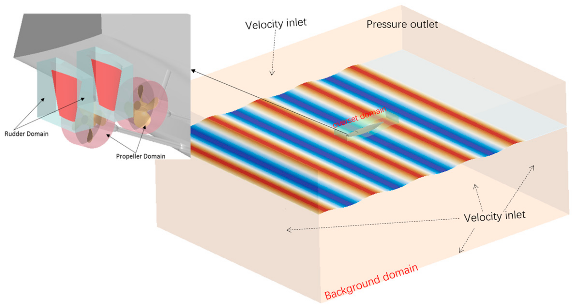
To improve the calculation of ship instability motions characterized by significant roll amplitudes, the overset grid module is utilized to fully couple the hull, propeller, and rudder system. As a result, the overall computational domain consists of six subdomains: one designated explicitly for the background grid (background domain), one for the grid surrounding the ship model (overset domain), two for the grids encompassing the propellers on the starboard and port sides (propeller domain), and two supplementary parts designated for representing the rudders on both sides (rudder domain).

Considering the ship instability motion in waves and the effects of wave reflection, the dimensions of the computational field are specified as follows: using the earth-fixed coordinate system as the reference at the initial moment, the background domain extends from −2.5 Lpp to 4.0 Lpp along the longitudinal axis of the ship, −2.5 Lpp to 2.5 Lpp in the direction of the transverse axis, and −2.0 Lpp to 1.0 Lpp in the vertical direction. The smaller overset domain is confined to the range of −0.15 Lpp to 1.2 Lpp in the direction of the longitudinal axis, −0.2 Lpp to 0.2 Lpp in the lateral direction, and −0.2 Lpp to 0.2 Lpp in the vertical direction.

In the background domain, the boundary condition of the pressure outlet is configured at the top of the ship, while all other boundaries employ velocity inlet conditions. Overset mesh conditions are imposed on all boundaries for the rest of the computational domain, and the fully appended ship geometry boundaries are given a no-slip condition. Figure 3 provides a comprehensive overview of the computational domain, encompassing the hull geometry and the types of boundary conditions.

The computational domain utilizes surface remesher and trimmer meshing techniques, incorporating prism layers along the wall boundaries. The grid topology of the entire computational domain is depicted in Figure 4.

The trimmer meshing approach primarily produces hexahedral cells within the domain, precisely trimming them based on the shape of the contact boundary surface. Adequate mesh refinement is applied in proximity to the bow, stern, and bilge keels of the hull. Specifically, the mesh size at the stern is uniformly refined due to the large roll amplitude induced by the pure stability failure. This roll can result in the propeller and rudder emerging from the water, causing substantial deformation and splashing around the free surface of the stern. Ensuring a high-quality mesh is imperative for averting computational divergence. The computational mesh undergoes progressive refinement in the proximity of the free surface, effectively capturing the intricate flow characteristics of the waves. Additionally, the prism layer mesher is utilized to create orthogonal prismatic cells along the walls. This aids in precisely estimating the near-wall flow, resolving the boundary layer, and capturing separated flow near the walls.

The total grid number for the free-running simulations in waves is around 11 million, and detailed mesh information in each part is listed in

Table 3. Mesh information for the free-running simulations in wave.

Item	Grid	Port	Starboard
Background	3.5 M	-	-
Hull	6.8 M	-	-
Propeller	0.5 M	0.25 M	0.25 M
Rudder	0.2 M	0.1 M	0.1 M
Total	11 M	-	-

.

3.3. Dynamic Ship Motion and Course-Keeping Method

To precisely simulate the realistic behavior of a ship, a Dynamic Fluid Body Interaction (DFBI) module is utilized, enabling the fully appended ship to move freely in 6-DOF. The simulation employs six distinct coordinate systems to carry out the 6-DOF motion, as illustrated in Figure 5. One coordinate system denotes the inertial earth-fixed system, another denotes the non-inertial ship-fixed system, two coordinate systems are assigned to the propellers, and two coordinate systems are designated for the rudders. It should be noted that the coordinate system shown in the CFD method may not align with the coordinate axis direction defined in the current potential flow method (as described in [9]). However, to compare results between the two methods, post-processing of motion results has been standardized by following the positive direction of various parameters as indicated in Figure 5.

The propellers and rudders exhibit a full 6-DOF motion synchronized with the ship while undergoing four additional rotations on both sides to coincide with the ship’s motion. The overset domain, encompassing the ship geometry, harmonizes with the hull. As a result, the background grids within the entire domain experience translations and rotations restricted to 3-DOF (surge, sway, and yaw) within the xoy plane, guaranteeing the correct alignment and positioning of the outer and inner computational domains throughout the simulation.

Feedback controllers control the speeds of self-propulsion and heading for maneuvers. A proportional integral (PI) controller modulates the propeller’s behavior, to attain the desired speed for the self-propulsion model in still water, as outlined in [21]. The control equation governing the speeds of the free-running model is formulated as follows:

$$n_{pro}=P\cdot e+I{\displaystyle {\int }_0^{t}edt}$$

(1)

$$e=U_{target}-U_{ship}$$

(2)

Here, n_pro represents the controller output, and e represents the difference in ship speed between the desired and the instantaneous values. P and I denote the proportional and integral gains, respectively.

To maintain the ship’s course in waves, a feedback controller regulates the rudder during the simulations of the self-propulsion motion. The control mechanism can be expressed by the following equation:

$$\dot{\delta }(t)=\left\{-\delta (t)-K_p(\chi (t)-{\chi }_c)\right\}/T_E$$

(3)

In the above equation, δ(t) represents the instantaneous rudder angle, χ(t) denotes the instantaneous heading angle of the ship, χ_c signifies the target yaw angle, K_p represents the proportional gain, and T_E represents the time step for rudder control. The target heading is maintained by adjusting the rudder angle at each time step.

3.4. Wave Generation and Absorption Method

A Stokes wave model with fifth-order theory was utilized to generate incident waves by prescribing the inlet velocity at the boundary.

A wave forcing model was introduced to reduce the computational domain size and efficiently attenuate the propagating waves at the boundaries of the background domain, as outlined in [24]. The wave forcing model was applied at the velocity inlet boundary, referred to as the forcing zone, to force the wave potential flow solution in the NS equations. Wave forcing is applied exclusively to the momentum equations by incorporating a source term in the following formula:

$$q_{\varphi }=-\gamma \rho \left(\varphi -{\varphi }^{\ast }\right)$$

(4)

where γ is the coefficient of wave forcing, $\varphi$ is the instantaneous solution of the current transport equation, ${\varphi }^{\ast }$ is the analytical solution for the region where the wave forcing model is applied, and ρ is the fluid density.

The source term of wave forcing is applied along all boundaries of the background domain, except for the top of the computational domain. This ensures that the solution in the wave-forcing zone is coerced toward the theoretical wave pattern, effectively suppressing the wave reflection. Figure 6 illustrates the changes in the strength of the forcing coefficient and the partitioning of the wave forcing region, with blue indicating the RANS zone and red representing the maximum forcing toward the Stokes fifth-order theory.

The strength of the wave-forcing model gradually transitions from 0 at the inner boundary of the wave-forcing zone to 1 at the outer boundary, indicating a gradual increase in the wave-forcing strength. The length of the wave forcing zone is also displayed in Figure 6.

4. Mathematical Model with Potential Theory

Pure stability failure is an extreme roll motion with strong nonlinear and a typical mode of stability failure in the new-generation IS criteria. To provide a software tool for evaluating the new-generation stability regulations of the intact ships, the stability research group at CSSRC developed a program called HydroSTAB-CSSRC. It encompasses a module for time domain prediction of pure stability failure in the seaway, developed by the second author [9,25]. For comparison with the CFD method, this study employs the strip method and a 6-DOF motion equation to simulate large roll motions during pure stability failure using HydroSTAB-CSSRC. The velocity potential is solved using the enhanced integral method. An instantaneous wetted surface integration approach is adopted to calculate the nonlinear Froude–Krylov roll restoring moment. The specific representation of the motion equation is as follows:

$$\left(m+A_{11}\right)\dot{u}-(m+A_{22}(u))vr=-R(u)+X_P+X_R(\delta )+F_1^{FK}({\xi }_G/\lambda ,\zeta ,\phi ,\theta ,\chi )$$

(5)

$$\left(m+A_{22}(u)\right)\dot{v}+\left(m+A_{11}\right)ur=Y_H+Y_R(\delta )+F_2^{FK}({\xi }_G/\lambda ,\zeta ,\phi ,\theta ,\chi )+F_2^{DF}({\xi }_G/\lambda ,{\chi }_C,u)$$

(6)

$$\begin{array}{l}(I_{xx}+A_{44})\dot{p}+(I_{xx}+A_{44})(2\alpha \cdot p+\gamma \cdot p^3)+A_{42}(u)\dot{v}+B_{42}(u)v+A_{46}(u)\dot{r}+B_{46}r+C_{46}(\chi -{\chi }_C)\\ =K_H+K_R(\delta )+F_4^{FK+B}({\xi }_G/\lambda ,\zeta ,\phi ,\theta ,\chi )+F_4^{DF}({\xi }_G/\lambda ,{\chi }_C,u)-W\cdot GZ({\phi }_0)\end{array}$$

(7)

$$\left(I_{zz}+A_{66}(u)\right)\dot{r}=N_H+N_R(\delta )+F_6^{FK}({\xi }_G/\lambda ,\zeta ,\phi ,\theta ,\chi )+F_6^{DF}({\xi }_G/\lambda ,{\chi }_C,u)$$

(8)

$$(m+A_{33}(u))\ddot{\zeta }+B_{33}(u)\dot{\zeta }+C_{33}\zeta +A_{35}(u)\ddot{\theta }+B_{35}(u)\dot{\theta }+C_{35}\theta =F_3^{FK}(u)+F_3^{DF}(u)$$

(9)

$$(I_{yy}+A_{55}(u))\ddot{\theta }+B_{55}(u)\dot{\theta }+C_{55}\theta +A_{53}(u)\ddot{\zeta }+B_{53}(u)\dot{\zeta }+C_{53}\zeta =F_5^{FK}(u)+F_5^{DF}(u)$$

(10)

$${\zeta }_G(t)={\zeta }_{Ga}(u)\cos [2\pi \cdot ({\xi }_G/\lambda )-{\delta }_3(u)]$$

(11)

$$\theta (t)={\theta }_a(u)\cos [2\pi \cdot ({\xi }_G/\lambda )-{\delta }_5(u)]$$

(12)

$${\xi }_G/\lambda =(u(t)\times \cos (\chi (t))-v(t)\sin (\chi (t))-C_W)\cdot t/\lambda$$

(13)

The subscripts H, R, and P refer to the hull, rudder, and propeller, respectively. Equations (5), (6), and (8) are the time domain maneuvering mathematical models of surge, sway, and yaw motions. Equation (7) is the time domain seakeeping mathematical model of the roll motion. Equations (9) and (10) are the frequency-domain seakeeping mathematical models of heave and pitch motions. The definitions of specific parameters in the above equations are as follows: m: ship mass; $u, v$: surge and sway velocity; $r$: yaw rate; $F_j^{FK}$: Froude–Krylov force in the j direction; $F_j^{DF}$: Diffraction force in the j direction; $\phi$: roll angle; $\theta$: pitch angle; $\zeta$: heave displacement; ${\xi }_G$: the distance of the ship’s center of gravity from the trough of a wave in the longitudinal direction; $\lambda$: wavelength; A_ij, B_ij, and C_ij are coupling seakeeping coefficients. The more details of the equations and parameters, refer to reference [25].

5. Results and Discussion

The following section presents the simulation results of the ONR tumblehome model in free-running conditions, specifically focusing on its behavior in the following seas using both CFD and potential flow methods. The course-keeping control of the free-running benchmark ONRT model is initially validated by the CFD method in the following waves. Subsequently, the simulation results of pure loss of stability obtained from different methods are compared and discussed. Additionally, an analysis is performed on the variation characteristics of the flow field around the ship model. The forces and moments acting on the appendages are shown during the ship’s capsizing process, which is triggered by pure stability failure at high speed.

5.1. Validation of the Course-Keeping Simulation Using the CFD Method

The accuracy of the free-running self-propulsion simulation, involving full 6-DOF motion in still water and course-keeping in waves, has been previously validated by Zeng et al. [26], specifically for head and bow quartering waves. Expanding on the groundwork laid by these previous studies, this paper additionally validates the maneuverability motion under course-keeping control in free-running mode with following waves.

For this subsection, we refer to the benchmark Case 3.13 presented in the ship hydrodynamics CFD workshop of Tokyo 2015. The simulation is carried out at a sailing speed of 1.11 m/s, corresponding to Fn = 0.2. The incident wave condition is set at H_w/λ = 0.02, λ/L_wl = 1.0, where λ is the wavelength, L_wl is the length of the waterline, and H_w represents the wave height. The propeller rate of revolution remains constant and is determined using the self-propulsion simulation conducted in calm water. The time step is configured at (0.0005 s), equating to roughly 1.5 degrees per time step for the rotation of the propeller.

The comparative results of the CFD and EFD are all expressed in a non-dimensional format. For the 6-DOF motions, the trajectory of motion is expressed as $\left(\left(X-X_0\right)/L_{wl},\left(Y-Y_0\right)/L_{wl}\right)$, time domain data of heave motion are described as $Z/{\zeta }_a$, where ${\zeta }_a$ is the wave amplitude. Three angular motions are presented as $\left(\varphi ,\theta ,\left(\psi -{\psi }_C\right)\right)/k{\zeta }_a$, where k is the wave number, $\varphi ,\theta ,\psi$ present the angles of roll, pitch and heading, respectively. ${\psi }_C$ is the target yaw angle. The longitudinal forward speed is normalized as $u=\dot{x}/V_A$, where $V_A$ is the target speed. The translations of the ship’s motion are reported in an Earth-fixed coordinate system, and the angular motions of the ship are presented in a ship-fixed coordinate system.

Figure 7 compares the simulation and experiment of ship motion in the following waves. The wave force acts symmetrically on the hull in following waves, resulting in minimal amplitudes of roll and yaw. The ship effectively maintains its course with the assistance of rudder control. The numerical calculation results for time histories of pitch and heave in the following wave exhibit good agreement with the test results. The heave motion slightly underestimates the test results, whereas the pitch motion closely aligns with the experimental measurements. The errors in the amplitudes of the first harmonic Fourier Series (FS) for heave and pitch motion are 14.37% and 5.05%, respectively.

The time history curve of the ship’s speed exhibits periodic fluctuations caused by the wave action in the following waves. The speed curve oscillates around the target speed as the ship encounters waves. Data from the stable section (after 2 s of unsteady behavior) following deceleration are considered for analytical purposes. The 0th harmonic FS term of the calculated forward speed (mean values) shows an error of 1.33% compared to the experimental data. The overall agreement demonstrates that the current approach for course-keeping control accurately captures the ship’s behavior in following waves.

5.2. Self-Propulsion of Free-Running Model in Calm Water

Before simulating the pure stability failure in the following waves, a self-propulsion simulation is conducted with a full 6-DOF motion under the automatic control of the rudders in calm water.

This simulation aims to determine the constant propeller rate of revolution at various target speeds. Figure 8 illustrates the results of the experiment and CFD simulation for the propeller rate of revolution when the free-running model reaches a stable target speed. The simulation outcomes for the fully appended vessel at various velocities conform to the test data, with an average discrepancy within 3%, as presented in

Table 4. Error between experimental data and CFD results of rotational rate of propellers.

Fn	Exp	CFD	Error
0.25	9.72	9.08	6.61%
0.275	10.53	10.62	−0.79%
0.30	12.15	11.87	2.33%
0.33	13.60	13.18	3.09%

. Figure 9 presents the wave pattern at different speeds. The wave elevation becomes pronounced with increasing ship speed, particularly at the bow and stern wave zones of the ship model.

5.3. Comparison of the Maximum Roll Amplitudes with Different Methods

The paper presents a comparative analysis of maximum roll amplitudes on the two sides of the ship model, utilizing various methodologies and then contrasting them with experimental data, as depicted in Figure 10. In the figure, the potential flow method yields results for both 4-DOF (Sim_lu (HydroSTAB)_4DOF, surge-roll-heave-pitch) and 6-DOF (Sim_lu (HydroSTAB)_6DOF) calculations. Another set of 6-DOF calculations based on potential flow theory accounts for the effect of the rudder and propeller emerging from the water by considering alterations in the effective underwater area. All results from the potential flow method are based on an initial heel angle of 8.6 degrees, with calculated velocities encompassing Fn = 0.25, 0.275, 0.3, 0.31, 0.32, and 0.33. In addition to scenarios that align with the experimental results, the CFD method’s computations encompass two supplementary sets of results. The first set pertains to an initial heel angle of 7.5 degrees at Fn = 0.3, and the second set involves an initial heel angle of 6 degrees at Fn = 0.33.

Considering the results of the CFD method, it is evident that, at Fn = 0.3, the vessel approaches a critical point of potential capsizing. Notably, variations in the initial heel angle have a pronounced influence on the vessel’s maximum roll amplitude. With the initial heel angle reduced to 7.5 degrees, the maximum roll angle is only 50.8 degrees, lower than the experimental value, and does not lead to capsizing. However, at Fn = 0.33, the vessel still capsizes even with a reduced initial heel angle of 6 degrees. This indicates that at this point, the sailing speed causes the vessel to stay near the wave crest for a longer duration, intensifying the phenomenon of pure stability failure. Despite the reduction in the initial constant roll angle, it is still difficult to counteract the insufficient restoring force caused by the waves, ultimately resulting in capsizing.

The computational data of the potential flow method show that at the critical speed Fn = 0.3, the results from different potential flow methods are all lower than the experimental data. However, it is noteworthy that these outcomes do not lead to capsizing at Fn = 0.3, in contrast to the findings obtained by the CFD method. Furthermore, whether the 6-DOF calculations consider the effects of the rudder and propeller exposure to water or not, there are negligible discrepancies in the maximum roll amplitude results. At the same time, in the 4-DOF calculations, beyond Fn = 0.32, the positive maximum roll amplitude gradually approaches approximately 10 degrees without reaching the point of capsizing, indicating the potential transition of the vessel into a stable equilibrium state.

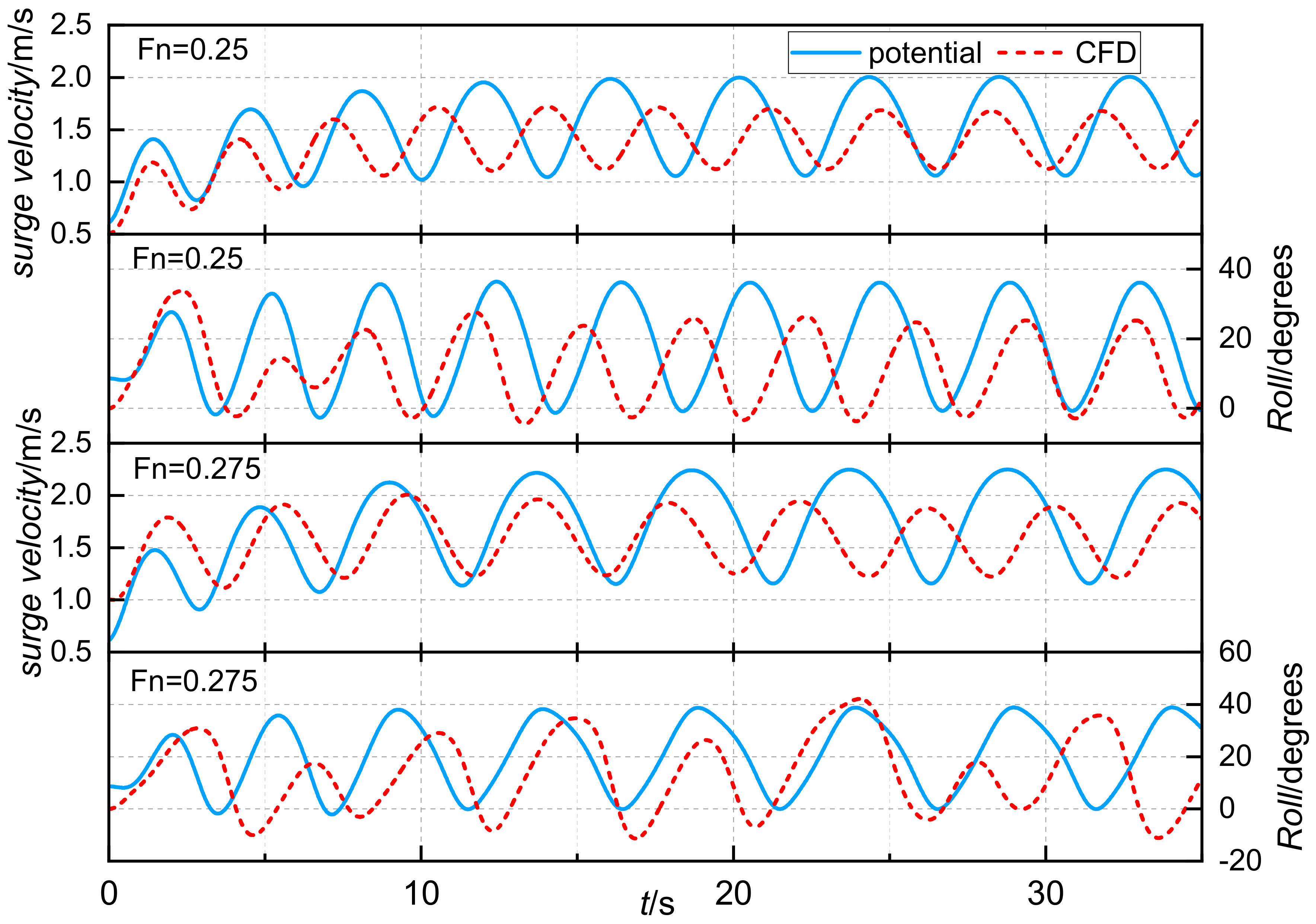
Figure 11 provides a comparison of the time histories of longitudinal velocity and roll angle calculated by the CFD method and the potential flow method at Fn = 0.25 and 0.275. From the graph, it can be observed that the ship’s velocity computed by the CFD method is lower than that obtained through the potential flow method, resulting in a smaller encountered period calculated by the CFD method. At Fn = 0.25, the ship exhibits stable periodic roll motion. The roll amplitude calculated by the CFD method is smaller than that by the potential flow method. However, at Fn = 0.275, it is evident that the CFD method yields unstable roll motion, and the potential flow method still shows stable roll motion. This indicates that the current potential flow model is unable to fully capture certain nonlinear motion phenomena.

5.4. Comparison of Typical Motion Processes for Pure Loss of Stability

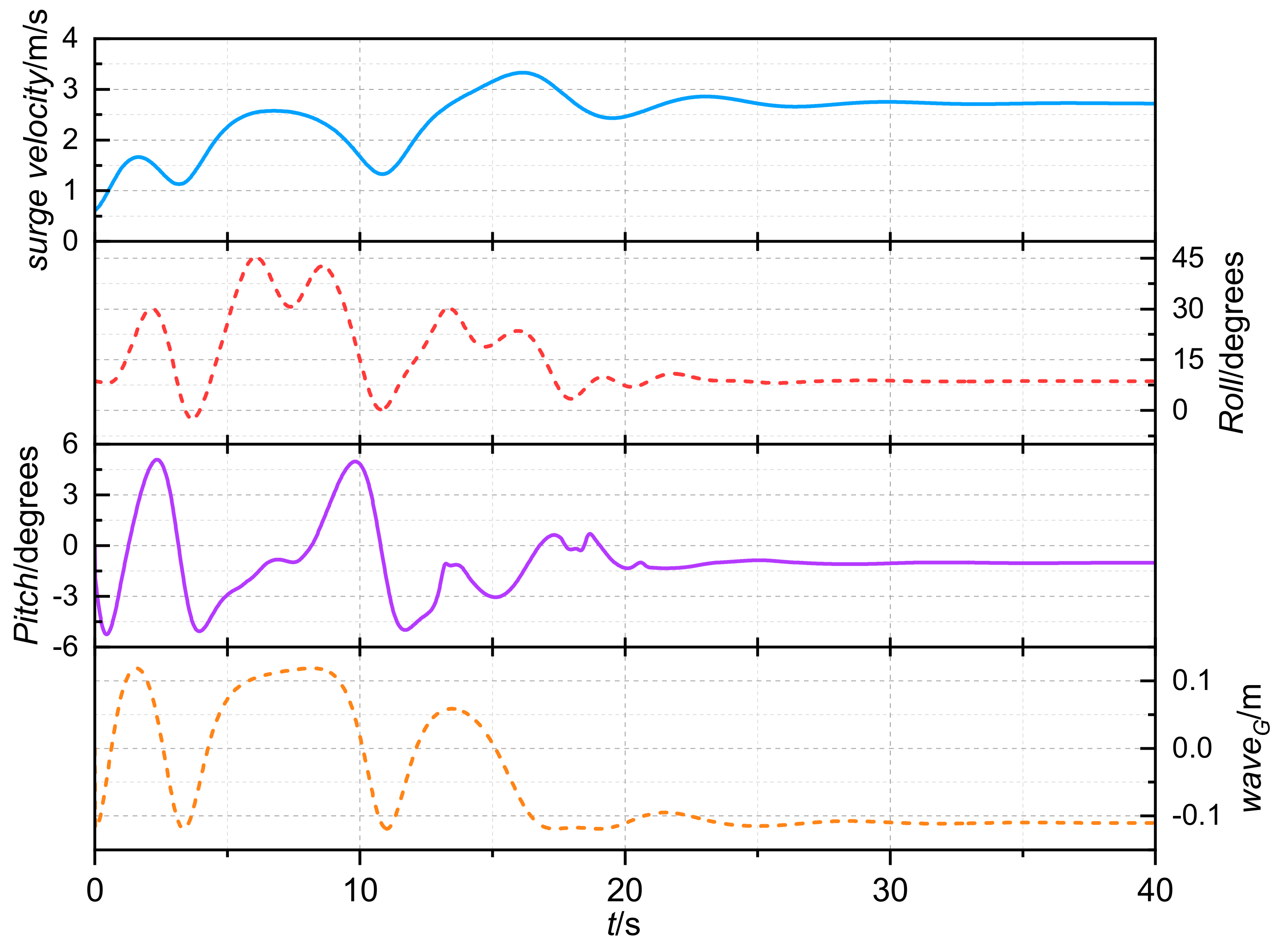
This section further analyzes the typical motion processes of pure loss of stability calculated using different methods. Figure 12 displays the motion time history obtained from the 4-DOF potential flow method at Fn = 0.33. In the previous analysis in Figure 10, it was observed that both experimental data and the 6-DOF computations indicated a capsizing event at this velocity. However, with the 4-DOF calculation, the vessel eventually reached a stable equilibrium state. Figure 12 shows that as the ship’s speed increases, it approaches the wave velocity. The duration of the vessel staying on the wave crest also gradually increases. During this period, inadequate restoring force leads to a significant roll angle of the ship (observed in the interval of 5–10 s). As the speed continues to increase due to the absence of yaw motion interference, the ship’s speed aligns with the wave celerity. The vessel stabilizes at an approximately 10-degree roll angle within this time interval, and the center of ship gravity is positioned near the wave trough with a stable trim of stern up. The ship and the wave remain in a state of stable surf-riding equilibrium in terms of their relative position.

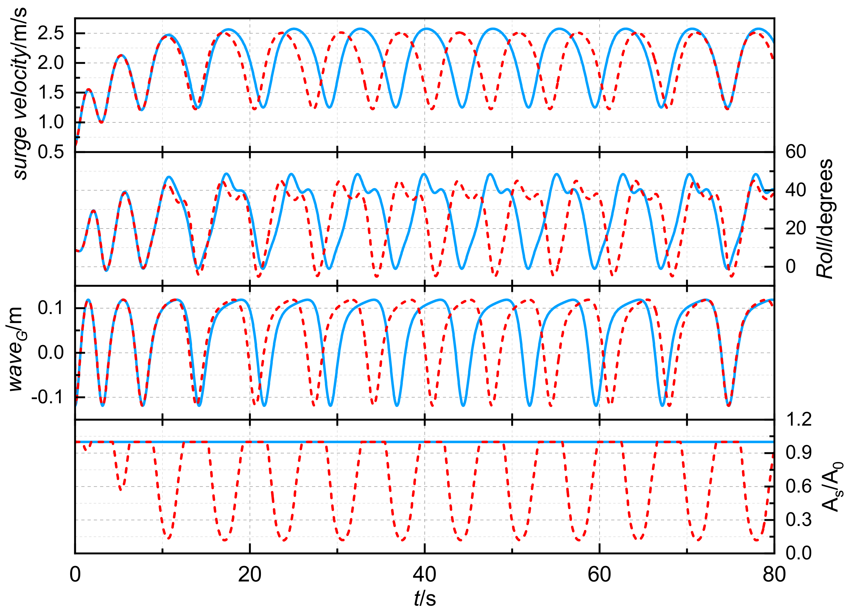
Figure 13 presents a comparative analysis of the time domain data of the motion obtained using the 6-DOF potential flow method at Fn = 0.3. The calculations were performed with and without considering the emerging from the water of the rudders and propellers (referred to hereafter as 6-DOF_wRP and 6-DOF_woRP, respectively). From the graph, it is evident that during the initial acceleration phase, both methods show consistent variations in speed and motion. As the speed gradually increases, the vessel’s roll amplitude also rises. When considering the 6-DOF_wRP method, the starboard propeller experiences partial exposure to water due to the significant roll amplitude. Consequently, the ratio of the wetted surface area to the disc area of the propeller changes with the roll motion. However, when considering the 6-DOF_woRP method, the ratio of the wetted surface area of the propeller remains constant at 1.

From the variation in surge velocity in Figure 13, it can be observed that accounting for the emerging from the water of the propellers leads to a reduction in thrust, resulting in a slightly lower peak velocity during the stable phase compared to the calculation using the 6-DOF_woRP method. When utilizing the 6-DOF_woRP method, the vessel remains at the wave crest longer due to the higher velocity, resulting in an extended encounter duration. In the end, both surge velocity and roll display stable periodic fluctuations, with roll motion exhibiting a nonlinear double-peak phenomenon near the maximum roll angle.

The CFD calculation results were selected for analysis at Fn = 0.3 and an initial heel angle of 7.5 degrees to enable comparison with the potential flow method. The corresponding time history curve of the ship’s motion is displayed in Figure 14. It can be observed that as the ship’s speed increases, the duration of the vessel staying near the wave crest gradually lengthens. Both the roll angle and roll period also increase gradually, particularly around 20 s, where the roll angle reaches its peak and the roll period is larger compared to the 10–15 s interval. When experiencing a maximum roll of approximately 50 degrees, the propeller on the starboard of the vessel is already entirely out of the water, indicating a significant decrease in speed due to reduced propulsion. As the ship’s speed decreases, the stability of the vessel gradually recovers, followed by a rapid reduction in the maximum roll amplitude to 30 degrees in the next cycle. The reduction in roll amplitude is accompanied by a gradual recovery of propulsion, increasing speed as the vessel continues into the next cycle of rolling.

At Fn = 0.3, the roll motion calculated by the 6-DOF potential flow method displays stable periodic fluctuations. In contrast, the roll motion computed using the CFD method is unstable. Additionally, at the maximum roll angle, the CFD method shows a significant reduction in the peak of surge velocity due to the effect of propeller exposure to water. This phenomenon was not observed in the potential flow results, where the surge velocity, like the roll motion, also displays stable periodic fluctuations. This indicates that for the large-amplitude coupled motions involving the interaction of hull, propeller, and rudder, the current potential flow models are not yet able to effectively capture the motion nonlinearity induced by specific, strong nonlinear factors.

Figure 15 and Figure 16 illustrate the time-varying curves of propeller torque and thrust at different sailing speeds. From the graphs, it can be observed that as the sailing speed increases, both the thrust and torque of the propellers also increase. Due to the initial left inclination, the propeller on the port side remains submerged chiefly, resulting in a higher overall thrust compared to the starboard propeller. Particularly when the roll angle is large, the starboard propeller emerges from the water, leading to a noticeable decrease in thrust.

5.5. Analysis of the Flow Field during a Typical Capsizing Process of Pure Loss of Stability

To further analyze the flow field variations during the capsizing process following pure stability failure, this study focuses on a computational case with Fn = 0.33 and an initial heel angle of 6 degrees using the CFD method. Figure 17 displays the time history curves of the ship’s roll angle and sailing speed. Figure 18 presents the time history curves of the propellers and rudders’ longitudinal forces, roll moment, and yaw moment. Four specific moments, labeled a, b, c, and d, are selected for analysis. 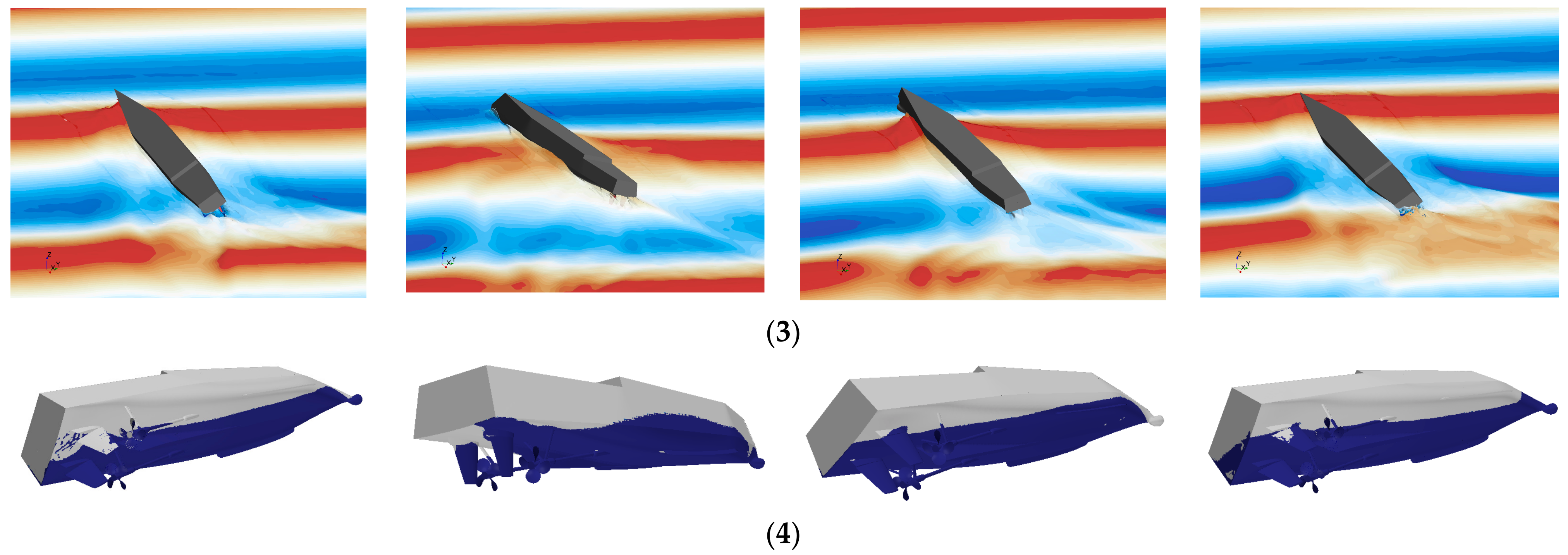In Figure 19, axial velocity profiles ahead of the propeller, pressure distributions on the aft hull and appendages, the ship’s motion attitude on the wave surface, and the wetted surface area distribution of the ship hull and appendages are depicted as contour maps corresponding to these four moments.

Figure 17 shows that the ship capsizes after two cycles of rolling. At point a, which represents a specific moment when the ship is approaching the first maximum roll angle, the ship’s relative position on the wave surface reveals that the wave crest is reaching the bow of the ship, and the ship is located on the upward slope of the wave. Insufficient stability leads to a significant roll angle. At this moment, the propeller on the starboard side of the ship partially emerges from the water, and the rotation of the propeller creates distinct curling wake patterns on the wave surface. The thrust generated by the port propeller is noticeably higher than that of the starboard propeller, as is evident from the pressure distribution on the propeller surfaces. At point a, the backflow surface of the starboard rudder is entirely out of the water, which is visible in the wetted surface contour map. This causes the longitudinal force, roll moment, and yaw moment generated by the starboard rudder to be smaller than those generated by the port rudder.

At point b, the ship has rolled to the maximum angle on the other side (approximately 10 degrees), and the sailing speed approaches the second peak. The velocity profile ahead of the propeller shows an increase in speed. At this moment, the wave crest is near the midship of the ship, and the reduced restoring force results in insufficient stability, causing the ship to transition into the next maximum roll motion. Both the port and starboard rudders and propellers are submerged, and the difference in forces and moments between them is not significant.

As the ship continues rolling toward the port side, at point c, the roll angle reaches approximately 20 degrees. The starboard propeller and rudder are on the verge of emerging from the water, and the wave crest gradually moves toward the bow of the ship, leading to a decrease in sailing speed. The roll moment and yaw moment generated by the port rudder are slightly greater than those generated by the starboard rudder. As the ship leans to the left, the pressure on the left side of the appendage supports and the pressure on the left side of the propeller blade surface increase compared to the right side.

Considering point d, the ship reaches the second maximum roll angle, and the wave trough is located at the midship of the ship. The restoring force increases and stability gradually recovers, causing the ship to start rolling back toward the starboard side. With the increasing roll angle, the pressure on the left side of the ship’s hull and appendage surface further increases.

6. Conclusions

This study utilizes the RANS method to analyze the phenomenon of pure stability failure in self-propelled ships under regular following waves at different sailing speeds. Additionally, it conducts comparisons and analyses with experimental data and calculations utilizing the potential flow method. The key findings are as follows:

• The established CFD method demonstrates good predictive accuracy for simulating course-keeping under regular waves.
• The established method can qualitatively predict the occurrence of pure stability failure. However, compared to potential flow methods, the CFD approach requires more computational time and is challenging to achieve quantitative analysis.
• The CFD method enables real-time consideration of propeller and rudder exposure from the water during large roll motions. For a ship with twin propellers and twin rudders, propeller and rudder exposure from the water will lead to an imbalance in forces and a reduction in thrust, resulting in a decrease in ship speed and a significant reduction in the maximum roll angle of the subsequent roll cycle. However, current potential flow models are still unable to capture such nonlinear phenomena accurately.
• Near the critical sailing speed for capsizing (Fn = 0.3), the maximum roll angle is highly sensitive to changes in the initial heel angle. Further analysis is needed to comprehend the factors influencing the prediction of the maximum roll angle near the critical capsizing speed.

Overall, the CFD method can be beneficial for improving potential flow models and enhancing the understanding of the physical mechanisms for instability motion. The research can expand to more complex wave motions, such as oblique waves, and consider a simplified propeller model by using body force to improve computational efficiency.