Abstract
In the paper, we analyze laser strainmeter data for the period from 2014 to 2022 to identify deformation anomalies that led to the generation of tsunamis in the area of the Japanese Islands. It is impossible to determine the main characteristics of a tsunami from the deformation anomaly registered by the laser strainmeter, but it is possible to calculate the seabed displacement in the epicenter of a tsunami formation, which causes the tsunami. We have established that the relationship between the registered deformation anomalies and the seabed displacement in the tsunami source in the area of the Japanese Islands is similar to the same relationships found in other regions of the Earth (Indonesia, Latin America, and the West Coast of North America). This result allows us to assert that such a relationship should be typical of any region of the Earth. The obtained results are aimed at solving the problem of reliable short-term tsunami forecasting, which allows for the avoidance of false alarms that lead to significant socio-economic damage.
1. Introduction
A tsunami is one of the most dangerous catastrophic phenomena on Earth. One of the regions of the planet affected by tsunamis the most is Japan. To detect and prevent this catastrophic phenomenon, a network of GPS receivers, seismic stations of ground and bottom types, and high-precision sea level meters has been developed on the islands and in the waters of Japan. In recent years, tsunami early warning systems have been widely introduced [1,2]. The development of remote satellite sensing of the water surface of tsunamis in tsunami-hazardous regions has led to the creation of the coastal Global Navigation Satellite System (GNSS), which applies an innovative method of reflecting signals that measure the height of the sea surface with high accuracy [3,4].
The Japan Meteorological Agency (JMA) plays the role of the Japan tsunami warning center; by analyzing seismic data, it gives a tsunami warning within 3 min [5]. To predict the consequences of a tsunami, JMA used an automatic monitoring method based on an estimation of the earthquake magnitude and its hypocenter location. However, after the tsunami in Tohoku in 2011, when JMA failed to predict the tsunami [6], a network of ocean-bottom seismometers (OBS) and tsunami sensors around the Japan Trench was created to improve the accuracy of tsunami forecasting [7,8,9]. Based on JMA data, many methods of tsunami estimation and forecasting were developed. Thus, using data on pressure on the ocean floor observed from the sensors (S-net), a method for estimating tsunamis in almost real-time mode was developed [10]. JMA has an enormous seismic and metrological database, used by many scientists for various studies unrelated to forecasting and estimating the impact of tsunamis [11,12]. Based on JMA data, a seismic method was developed for use in tsunami warning that is based on the detection of the W-phase that appears between P-waves and S-waves in seismic records. This method is used to estimate seismic moments, epicenter location, and fault mechanism. It was demonstrated in many works and is actively used by tsunami warning centers [13,14].
Seismic methods of tsunami forecasting include, to a certain extent, the deformation method, which is based on determining the magnitude of the seabed displacement leading to the occurrence of a tsunami. This displacement can happen both as a result of an earthquake and as a result of an underwater landslide, volcanic activity, and the collapse of rock masses into the sea. The essence of this method is to identify a deformation anomaly on the records of laser strainmeters. The value of such an anomaly, taking into account the distance from the place of registration to the source of tsunami formation, is proportional to the displacement of the seabed at the tsunami source, which leads to the formation of a tsunami. For the first time, a deformation anomaly (deformation jump) was detected on the record of the device during the registration of the catastrophic tsunami of 2004 in Indonesia [15]. Deformation anomalies have been recorded during many tsunamigenic earthquakes. The deformation method proved its worth in estimating the tsunamigenicity of earthquakes in various regions. Using this method, we analyzed the records of earthquakes that occurred between 2010 and 2018 in three tsunami-hazardous areas: Indonesia, Chile, and the western coast of North America. For each of these regions, large earthquakes were selected with a magnitude of more than 7.5 and a depth of no more than 50 km, after which a tsunami was registered [16]. The results of the studies described in [16] allow us to determine with great accuracy the value of the seabed displacement, which leads to the generation of a tsunami. Based on this important result, it is possible to construct an adequate working model of an emerging tsunami, which is important for its monitoring and assessment of its impact on natural and artificial objects.
For the Japanese region, such an analysis has not been carried out. It is important to find out whether there is a relationship between the magnitude of the deformation jump registered by the laser strainmeter and the magnitude of the seabed displacement in the area of a tsunami source. Is it the same as in other regions of the Earth or different?
The task is solved based on the analysis of the records of a laser deformograph located at the coordinates 42°34.798′ N 131°9.400′ E (south of the Primorsky Territory of the Russian Federation). The choice of this equipment is associated with its unique amplitude-frequency characteristics, which make it possible to measure the deformations of the Earth’s crust at its locations with an accuracy of fractions of nanometers in a wide frequency range (from 0 conditionally to 1000 Hz). Currently, laser deformographs are successfully working, solving various fundamental and applied problems [17,18,19,20]. Taking into account the unique amplitude-frequency characteristics, laser deformographs, the optical scheme of which is based on the Michelson interferometer, are the best installations for recording signals in low-frequency and ultra-low-frequency ranges. Any broadband seismographs are unsuitable for solving this task due to the limitations of their operating frequency range from below (i.e., in the region of ultra-low frequencies), and GPS receivers have low sensitivity.
2. Description of the Used Equipment and the Obtained Experimental Data
To register deformation anomalies, we use a laser strainmeter due to its unique amplitude-frequency characteristics, which allow us to register the anomalies at almost any planetary distance. The laser strainmeter, the records of which were processed before preparation of this paper, is a part of the seismoacoustic and hydrophysical complex located on the territory of the International Scientific and Educational Site of the POI FEB RAS “Shultz Cape” [21], Figure 1. The instrument is installed at the point with coordinates 42°34.798′ N, 131°9.400′ E. It is based on an unequal-arm Michelson interferometer with a measuring arm length of 52.5 m, which is oriented at an angle of 18° to the North-South line. It uses a frequency-stabilized helium-neon laser by Melles Griott with a long-term stability of 10−9 as a light source. The device is located in a thermally insulated underground room at a depth of more than 3 m under the Earth’s surface, at an altitude of about 60 m above sea level. The operating frequency range of the laser strainmeter extends from 0 (conditionally) to 1000 Hz. The applied interferometry methods allow measuring the displacement at the base of the instrument with an accuracy of 10 pm. Data from the laser strainmeter and other devices is transmitted via cable lines to the recording computer, where, after pre-processing, it forms the files with a duration of 1 h and a sampling frequency of 1000 Hz. Depending on the tasks to be solved, the sampling frequency can be increased up to 10,000 Hz. Data from the laser strainmeter and other devices forms an experimental database, which is continuously updated. Data from all instruments in the complex is synchronized according to the “Trimble 5700” exact time clock. Figure 2 shows the layout of the laser strainmeter and broadband seismograph installation, which are parts of the complex. The broadband seismograph “Guralp CMG-3ESPB”, shown in Figure 1, consists of three sensors that allow recording ground oscillations simultaneously in three directions: “North-South”, “West-East”, and vertically. The frequency range of each sensor is 0.003–50 Hz. An analog signal after digitization by a 24-bit “GeoSIG GSR-24” ADC is transmitted to the recording device. The broadband seismograph, like the laser strainmeter, is located in a thermally insulated room at a depth of 3 m from the Earth’s surface. It is used to register earthquakes, but due to the limited operating frequency range, it cannot register the observed deformation anomalies described in [16] and further described in this paper. The seismoacoustic and hydrophysical complex is located far from highways and infrastructure facilities, which allows for more accurate and reliable seismic observations without extraneous noise.
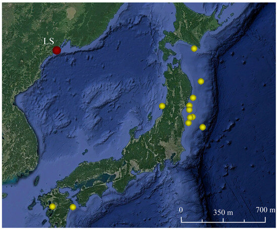
Figure 1.
Schematic map of the location of instruments (red circle) and earthquake epicenters (yellow circles).
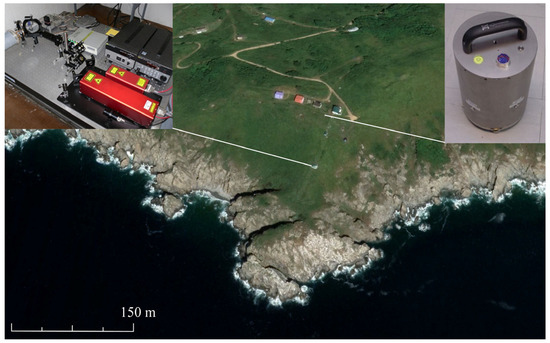
Figure 2.
Device installation layout.
We used the data presented on the website of the U.S. Geophysical Survey [22] as theoretical estimates of the seabed displacement in the place of tsunami generation. In total, in the period from 2014 to 2022, 12 records of earthquakes near the Japanese Islands were selected, with magnitudes greater than 6 (see Table 1) and at a depth of no more than 50 km, which were classified as tsunamigenic by the relevant services. The selection of the material for analysis was carried out as follows: (1) at the first step, for the period from 2014 to 2022, we selected the earthquakes marked on the website of the American Geophysical Survey as potentially tsunamigenic; (2) at the second step, we left only those earthquakes that formed during the laser strainmeter operation; (3) the comparison of the deformation anomaly magnitude in the records of the laser strainmeter with the seabed displacement magnitude in the tsunami epicenter, obtained from model calculations, was performed only for those earthquakes for which such calculations had been carried out. We took the calculation results from the same source [22].

Table 1.
Data of tsunamigenic earthquakes in the period from 2014 to 2022.
Next, let us analyze the laser strainmeter records containing information on these earthquakes.
3. Methodology
Any earthquake occurring in oceanic or continental-type crust generates oscillations, the frequency range of which depends on the characteristics of the source area and the length of the rupture in the hypocenter [16,23]. The magnitudes of these oscillations’ periods are very closely related to the magnitudes of the earthquakes. The greater the length of the rupture—the greater the magnitude—the greater the periods of oscillations that occur in the source area. As a rule, the periods of these oscillations start in the first ten seconds and end within the first few minutes. These oscillations never cause, and cannot cause, a tsunami. Tsunamis are caused by secondary consequences of earthquakes: an abrupt displacement of the seabed over relatively large areas; huge landslides that occur during underwater and continental-coastal earthquakes; the collapse of large masses of rocks into water, etc. It is clear that the cause of a tsunami is the displacement of these masses of the Earth’s crust in a very short period of time. If we can register these displacements, we can talk about the danger of a tsunami emergence. However, the main characteristics of emerging tsunamis also depend on many parameters (the depth of the sea at the place of displacement of the Earth’s crust segments, the nature of this displacement, etc.). Although if we talk about a tsunami as a wave in a bay, we can also note that in different bays where the tsunami will come, there will be different heights of the tsunami. However, we do not touch upon it in this paper. These results follow not only from theoretical but also from experimental works. As confirmation, Table 2 shows the seabed displacements in the source area of the tsunami and the heights of the tsunami waves that emerged due to them, taken from [16].
Table 2.
Calculated displacements in the focal area of the tsunami and deformation anomaly values recorded by the laser strainmeter.
Analyzing the results presented in Table 2, we can note the following: (1) the magnitude of the Earth’s sea crust displacement in the source area of a tsunami does not correlate with the maximum height of the tsunami; (2) the root cause of the tsunamis is these displacements, along with underwater landslides and the collapse of the masses of the Earth’s crust into the sea.
The advantage of this method is that deformation anomalies, characteristic of tsunamigenic earthquakes, propagate through the Earth’s crust at a speed several times greater than the tsunami speed. The systems whose operating frequency range allows recording these anomalies can remotely register such anomalies a short time after they occur. Based on the fact that such anomalies were registered after specific earthquakes, these earthquakes can be classified as tsunamigenic.
We recorded a deformation anomaly for the first time after the catastrophic tsunami in December 2004 in Indonesia. Similar deformation anomalies are also characteristic of tsunamigenic earthquakes occurring in the Japanese region. As a typical example, we will consider the laser strainmeter records of two earthquakes that occurred on 5 September 2004 on the southern coast of the island of Honshu, Japan. They are shown in Figure 3. The first earthquake with a magnitude of 7.2 occurred at 10:07:07 in the point with coordinates 33.14° N, 136.62° E, at a distance of about 75 km to the east of Honshu, at a focal depth of 20 km. The second earthquake with a magnitude of 7.5 occurred at 14:57:16. Its hypocenter was located at the point with coordinates 33.19° N, 137.05° E, at a distance of about 130 km to the east of the southern part of Honshu, at a focal depth of 10 km. Both of these earthquakes were recorded by the unequal-arm laser strainmeter, located at a distance of about 1162 km from the earthquakes’ epicenters. The signal of the first earthquake was registered at 10:13:46, and the signal of the second earthquake was registered at 15:03:52. Taking into account the distance from the earthquakes’ epicenters to the location of the laser strainmeter and the time of oscillation propagation, we get that their propagation speed is approximately equal to 2.909 km/s. By the magnitude principle, both of these earthquakes can be classified as tsunamigenic.
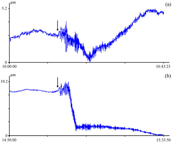
Figure 3.
Fragments of a 52.5-m laser strainmeter record of 5 September 2004, Honshu. UTC time. The first earthquake with a magnitude of 7.2 occurred at 10:07:07 (a), the second earthquake with a magnitude of 7.5 occurred at 14:57:16 (b). The arrow indicates the moment of the beginning of the earthquake registration.
Figure 4 shows an enlarged record of the unequal-arm laser strainmeter of the first earthquake and the dynamic spectrogram of this earthquake. The arrow marks the beginning of the earthquake registration. The record at the time of earthquake registration does not show any deformation anomalies, peculiar for tsunamigenic earthquakes, and the dynamic spectrogram clearly shows oscillations with periods of about 10 and 16 s, with amplitude greater than oscillations in the low-frequency range. The absence of a deformation anomaly indicates that this earthquake is not tsunamigenic.
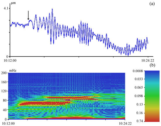
Figure 4.
Fragment of a 52.5-m laser strainmeter record of a non-tsunamigenic earthquake (a) and a dynamic spectrogram of this earthquake (b). UTC time. The arrow indicates the moment of the beginning of the earthquake registration.
Figure 5 shows a record of the unequal-arm laser strainmeter of the second earthquake and the dynamic spectrogram of this record. The arrow marks the beginning of the earthquake registration. Analyzing the record, we found a change in its nature—a deviation from the trend (red line). This is the deformation anomaly that occurred about 2.5 min after the earthquake’s onset. The deformation anomaly magnitude on the base of the laser strainmeter with a 52.5-m measuring arm was about 19.2 μm. The dynamic spectrogram contains oscillations with periods of 10 and 16 s. What can we say when comparing these earthquakes? In magnitude, they are approximately equal; the periods of oscillations that have been generated in the hypocenter of earthquakes are surprisingly the same. If we do not take into account the specified deformation anomaly, then it is difficult to relate one of these earthquakes to being tsunamigenic and the other to being non-tsunamigenic. Nevertheless, after the first earthquake, a tsunami did not occur, but after the second one, it did. It follows from the above that one of the two earthquakes can be classified as tsunamigenic only on the grounds of a deformation anomaly.
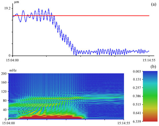
Figure 5.
Fragment of a 52.5-m laser strainmeter record of a tsunamigenic earthquake (a) and a dynamic spectrogram of this earthquake (b). UTC time. The laser strainmeter record (blue), the trend line (red).
The tsunamigenic earthquake that occurred on 5 September 2004 was in a place where the sea depth was approximately 2700 m. The distance from the earthquake’s epicenter to the nearest shore is 130 km; since a tsunami speed can be 0.16 km/s, the wave will reach the shore in 812 s. The laser strainmeter, installed 1162 km from the epicenter of the earthquake, registered the deformation anomaly 9 min before the time of arrival of the tsunami to the nearest coast [15].
4. Processing and Discussion of the Results Obtained
All earthquakes listed in Table 1 were classified as tsunamigenic by the tsunami warning services at the first step. The analysis of the laser strainmeter records showed that some of the above earthquakes were accompanied by the presence of such a deformation anomaly, and some other earthquakes were not.
As an example, let us consider the laser strainmeter records of two non-tsunamigenic earthquakes listed in Table 1. Figure 6 shows the laser strainmeter records of these earthquakes. As we can see in Figure 6, there is no deformation anomaly characteristic of a tsunamigenic earthquake. The 2014 earthquake happened 139 km from Namie at 37.005° N 142.453° E at 19:22:00 (UTC) on 11 July. The magnitude of the earthquake was 6.5, and its hypocenter was located at a depth of 20 km [24]. An enlarged fragment of the 2014 earthquake record and a dynamic spectrogram are shown in Figure 7. There is no deformation jump in Figure 7a. On the dynamic spectrogram in Figure 7b, there are oscillations with periods of 10 and 14 s. The absence of a deformation anomaly indicates that this earthquake is being non-tsunamigenic.
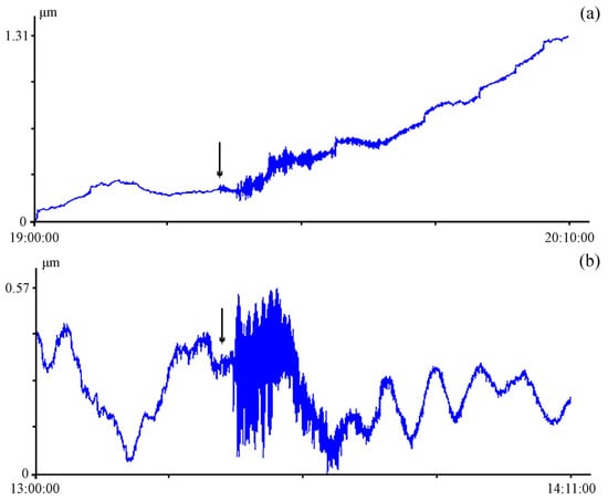
Figure 6.
Fragment of a 52.5-m laser strainmeter record of 11 July 2014, Namie (a) and 18 June 2019, Tsuruoka (b). UTC time. The arrow indicates the moment of the beginning of the earthquake registration.
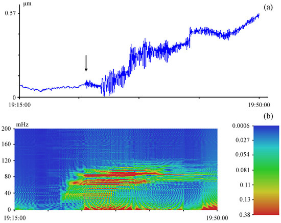
Figure 7.
Fragment of a 52.5-m laser strainmeter record of 11 July 2014, Namie (a) and dynamic spectrogram of this record (b). UTC time. The arrow indicates the moment of the beginning of the earthquake registration.
Figure 8a shows a fragment of the laser strainmeter record during the registration of the earthquake in 2018 (June). It happened on 18 June 2019 at 13:22:19 (UTC), 31 km from Tsuruoka, Japan. The magnitude of the earthquake was 6.4, and its hypocenter was located at a depth of 12 km [25]. The earthquake was classified as tsunamigenic. There is no deformation anomaly on this record, and for this reason it cannot be attributed to tsunamigenic, which was exactly the case. On the dynamic spectrogram in Figure 8b, oscillations with periods of 10 and 14 s are observed.
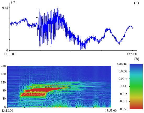
Figure 8.
Fragment of a 52.5-m laser strainmeter record of 18 June 2019, Tsuruoka (a) and dynamic spectrogram of this record (b). UTC time. The arrow indicates the moment of the beginning of the earthquake registration.
Let us consider the earthquakes from Table 1, which can be related to tsunamigenic earthquakes according to deformation features. Figure 9 shows fragments of the laser strainmeter records at the time of the registration of earthquakes in 2016 and 2021. Both of these earthquakes were classified as tsunamigenic. The figures show how the nature of the record changes at the moment of the earthquake: it deviates from the trend (red line). This deviation (deformation anomaly) is characteristic of tsunamigenic earthquakes. We will consider this deformation anomaly below.
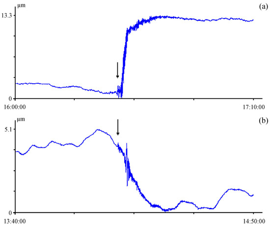
Figure 9.
Fragment of a 52.5-m laser strainmeter record of 15 April 2016, Kumamoto (a), and 13 February 2021, Namie (b). UTC time. The arrow indicates the moment of the beginning of the earthquake registration.
The earthquake shown in Figure 10 occurred at 16:25:06 (UTC) on 15 April 2016, 6 km from Kumamoto, Japan, at the point with coordinates 32.791° N 130.754° E. The magnitude of the earthquake is 7, and its hypocenter was located at a depth of 10 km [26]. Figure 10a shows a fragment of the laser strainmeter record at the time of registration of the tsunamigenic earthquake. We can see from the graph that a deformation anomaly occurred a few seconds after the onset of the earthquake, the magnitude of which in the laser strainmeter record was 8.4 μm. On the dynamic spectrogram Figure 10b, oscillations with periods from 10 to 14 s stand out.
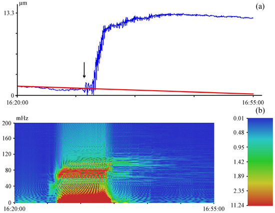
Figure 10.
Fragment of a 52.5-m laser strainmeter record of 15 April 2016, Kumamoto (a) and dynamic spectrogram of this record (b). UTC time. The laser strainmeter record (blue), the trend line (red). The arrow indicates the moment of the beginning of the earthquake registration.
The next earthquake, which, due to the presence of a deformation anomaly, can be related to tsunamigenic earthquakes, occurred on 13 February 2021 at 14:07:49 (UTC), 73 km from Namie, Japan, at the point with coordinates 37.727° N 141.775° E. The magnitude of the earthquake was 7.1, and the hypocenter was at a depth of 44 km [27]. The earthquake was recorded by the laser strainmeter; a fragment of this record is shown in Figure 11a. The magnitude of the deformation anomaly is 4.1 μm. Figure 11b shows the dynamic spectrogram of this record fragment, in which oscillations with periods of 10 and 14 s stand out. Due to the presence of a deformation anomaly, this earthquake can be classified as tsunamigenic.
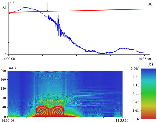
Figure 11.
Fragment of a 52.5-m laser strainmeter record of 13 February 2019, Namie (a) and dynamic spectrogram of this record (b). UTC time. The laser strainmeter record (blue), the trend line (red). The arrow indicates the moment of the beginning of the earthquake registration.
We will take the value of the deformation anomaly at the place of registration from the experimental data of the laser strainmeter and the calculated value of the seabed displacement from the website of the U.S. Geological Survey [22] since there are no instruments capable of registering this displacement on the seabed. The seabed displacements are calculated using a kinematic approach based on the Ji method [28]. In this method, both Rayleigh and Love surface waves and P and S surface waves are used for calculation. The values of deformation anomalies recorded by the laser strainmeter and the calculated displacements in the centers for earthquakes in 2016 and 2021 are presented in Table 3.
Table 3.
Calculated displacements and magnitudes of deformation anomalies, recorded by the laser strainmeter.
In accordance with [25], let us calculate the degree of divergence for each of the considered tsunamigenic earthquakes using experimental and model data. The degree of divergence is understood as the degree α at the distance in the following formula:
where A is the displacement value, recorded by the laser strainmeter; A0 is the value of the calculated displacement at a distance of 1 m from the conditional epicenter of the earthquake; R is the distance from the earthquake generation site to the laser strainmeter; and α is the degree. Hence, α = 1/2 means a drop in the amplitude of the signal according to the cylindrical law, and α = 1 means a drop in the amplitude of the signal according to the spherical law. Therefore, the numerator dimension is in meters, and the denominator is also in meters.
Taking into account that the distance from the epicenter of the earthquake of 15 April 2016 to the place of the unequal-arm laser strainmeter installation was about 1081 km, the degree of divergence is α = 0.941 obtained from Kumamoto data. The epicenter of the second earthquake, which occurred on 13 February 2021, was almost 893 km away from the place of the laser strainmeter installation. The degree of divergence for it is equal to α = 0.952 obtained from Namie data. In this case, as in the data presented in [29], the calculated degree of divergence is close to spherical, but it is not spherical. The results obtained for earthquakes that occurred near Japan are in very good agreement with the results obtained earlier for other tsunamis in tsunami-hazardous regions.
The use of laser strainmeter data allows not only to determine whether an earthquake is tsunamigenic or not but also to quickly obtain an approximate value of the displacement in the epicenter. Knowing the location of the epicenter, the depth of the sea, this value, and other factors, it is possible to determine the magnitude of a tsunami for a particular area. This will minimize damage and increase the stability of buildings and structures when a wave comes ashore. Using the calculations given in [30,31] and the model of tsunami propagation, as well as statistical data, it is possible to reduce the destruction when the wave comes ashore.
5. Conclusions
When analyzing the records of the laser strainmeter, we found that tsunamigenic earthquakes in the Japanese region are accompanied by deformation anomalies, the magnitude of which is closely related to the displacement of the seabed at the source of tsunami formation. In this case, the magnitude of the deformation anomaly that occurred in the tsunami source area decreases, almost according to the spherical law, with distance from the earthquake epicenter. This behavior of deformation anomalies generating tsunamis is also characteristic of other regions of the Earth, which indicates the universality of this phenomenon. Taking into account the displacement measurement accuracy at the base of the laser strainmeter, which is equal to 10 pm, we can assert that the laser strainmeter is able to record the displacement of the seabed in the source of tsunami formation at a distance of 20,000 km (half the length of the equator), equal to about 2 mm. Thus, even using a single laser strainmeter installed at any point on the Earth, it is possible to record the displacements of the seabed, which lead to the generation of a tsunami. To successfully solve the problem of determining the tsunamigenicity of earthquakes, model calculations are also required; their results, when compared with the obtained experimental results, will allow for the development of the most efficient methods for preventing the tsunami hazard.
Currently, the probability of a tsunami is associated with the magnitude of an underwater earthquake. This method, unfortunately, raises a lot of false alarms. False alarms lead not only to great economic damage but also to a negative social effect due to the fact that when a real tsunami wave occurs, the population may react to this message as another false alarm and fail to work out mandatory anti-tsunami measures. The results obtained in [16] and described in this article convince us of the effectiveness of the methods obtained in tsunami warning services, which will allow us to solve the problem of false alarms for any regions of the Earth when developing this method of automatism.
Author Contributions
G.D.—problem statement, discussion, and writing of the article. S.D.—data processing, discussion, and writing of the article. All authors have read and agreed to the published version of the manuscript.
Funding
The work was supported in part by the State Assignment under Grant AAAA-20-120021990003-3 “Investigation of fundamental bases of generation, development, transformation, and interaction of hydroacoustic, hydrophysical, and geophysical fields of the World Ocean”.
Institutional Review Board Statement
Not applicable.
Informed Consent Statement
Not applicable.
Data Availability Statement
Third-party data; restrictions apply to the availability of these data.
Acknowledgments
We would like to express our deep gratitude to all employees of the Physics of Geospheres laboratory.
Conflicts of Interest
The authors declare no conflict of interest.
References
- Percival, D.B.; Denbo, D.W.; Eble, M.C.; Gica, E.; Mofjeld, H.O.; Spillane, M.C.; Tang, L.; Titov, V.V. Extraction of tsunami source coefficients via inversion of DART® buoy data. Nat. Hazards 2011, 58, 567–590. [Google Scholar] [CrossRef]
- Boebel, O.; Busack, M.; Flueh, E.R.; Gouretski, V.; Rohr, H.; Macrander, A.; Krabbenhoeft, A.; Motz, M.; Radtke, T. The GITEWS ocean bottom sensor packages. Nat. Hazards Earth Syst. Sci. 2010, 10, 1759–1780. [Google Scholar] [CrossRef][Green Version]
- Tsushima, H.; Hino, R.; Ohta, Y.; Iinuma, T.; Miura, S. TFISH/RAPiD: Rapid improvement of near-field tsunami forecasting based on offshore tsunami data by incorporating onshore GNSS data. Geophys. Res. Lett. 2014, 41, 3390–3397. [Google Scholar] [CrossRef]
- Stosius, R.; Beyerle, G.; Helm, A.; Hoechner, A.; Wickert, J. Simulation of space-borne tsunami detection using GNSS-Reflectometry applied to tsunamis in the Indian Ocean. Nat. Hazards Earth Syst. Sci. 2010, 10, 1359–1372. [Google Scholar] [CrossRef]
- Tatehata, H. The New Tsunami Warning System of the Japan Meteorological Agency. In Perspectives on Tsunami Hazard Reduction: Observations, Theory and Planning. Dordrecht, Springer; Hebenstreit, G., Ed.; Springer: Berlin/Heidelberg, Germany, 1997; pp. 175–188. [Google Scholar] [CrossRef]
- Hosiba, M.; Ozaki, T. Earthquake Early Warning and Tsunami Warning of JMA for the 2011 off the Pacific Coast of Tohoku Earthquake. Zisin (J. Seismol. Soc. Jpn. 2nd Ser.) 2012, 64, 155–168. [Google Scholar]
- Sato, M.; Ishikawa, T.; Ujihara, N.; Yoshida, S.; Fujita, M.; Mochizuki, M.; Asada, A. Displacement above the Hypocenter of the 2011 Tohoku-Oki Earthquake. Science 2011, 332, 1395. [Google Scholar] [CrossRef]
- Kanazawa, T. Japan Trench Earthquake and Tsunami Monitoring Network of Cable-linked 150 Ocean Bottom Observatories and its Impact to Earth Disaster Science. In Proceedings of the 2013 IEEE International Underwater Technology Symposium (UT), Tokyo, Japan, 5–8 March 2013; pp. 1–5. [Google Scholar]
- Li, Y.; Goda, K. Hazard and Risk-Based Tsunami Early Warning Algorithms for Ocean Bottom Sensor S-Net System in Tohoku, Japan. Using Seq. Mult. Linear Regres. Geosci. 2022, 12, 350. [Google Scholar] [CrossRef]
- Inoue, M.; Tanioka, Y.; Yamanaka, Y. Method for Near-Real Time Estimation of Tsunami Sources Using Ocean Bottom Pressure Sensor Network (S-Net). Geosciences 2019, 9, 310. [Google Scholar] [CrossRef]
- Eum, H.-S.; Jeong, W.-M.; Chang, Y.S.; Oh, S.-H.; Park, J.-J. Wave Energy in Korean Seas from 12-Year Wave Hindcasting. J. Mar. Sci. Eng. 2020, 8, 161. [Google Scholar] [CrossRef]
- Hisaki, Y. Intercomparison of Assimilated Coastal Wave Data in the Northwestern Pacific Area. J. Mar. Sci. Eng. 2020, 8, 579. [Google Scholar] [CrossRef]
- Kanamori, H.; Rivera, L. Source inversion of W phase: Speeding up seismic tsunami warning. Geophys. J. Int. 2008, 175, 222–238. [Google Scholar] [CrossRef]
- Duputel, Z.; Rivera, L.; Kanamori, H.; Hayes, G.P.; Hirshorn, B.; Weinstein, S. Real-time W phase inversion during the 2011 off the Pacific coast of Tohoku Earthquake. Earth Planets Space 2011, 63, 535–539. [Google Scholar] [CrossRef]
- Dolgikh, G.I.; Dolgikh, S.G.; Kovalev, S.N.; Koren, I.A.; Ovcharenko, V.V.; Chupin, V.A.; Shvets, V.A.; Yakovenko, S.V. Recording of deformation anomaly of a tsunamigenous earthquake using a laser strainmeter. Dokl. Earth Sci. 2007, 412, 74–76. [Google Scholar] [CrossRef]
- Dolgikh, G.; Dolgikh, S. Deformation Anomalies Accompanying Tsunami Origination. J. Mar. Sci. Eng. 2021, 9, 1144. [Google Scholar] [CrossRef]
- Araya, A.; Takamori, A.; Morii, W.; Miyo, K.; Ohashi, M.; Hayama, K.; Uchiyama, T.; Miyoki, S.; Saito, Y. Design and operation of a 1500-m laser strainmeter installed at an underground site in Kamioka, Japan. Earth Planets Space 2017, 69, 77. [Google Scholar] [CrossRef]
- Jahr, T.; Kroner, C.; Lippmann, A. Strainmeters at Moxa observatory, Germany. J. Geodyn. 2006, 41, 205–212. [Google Scholar] [CrossRef]
- Takamori, A.; Araya, A.; Miyo, K.; Washimi, T.; Yokozawa, T.; Hayakawa, H.; Ohashi, M. Ground strains induced by the 2022 Hunga-Tonga volcanic eruption, observed by a 1500-m laser strainmeter at Kamioka, Japan. Earth Planets Space 2023, 75, 98. [Google Scholar] [CrossRef]
- Zurn, W.; Ferreira, A.M.G.; Widmer-Schnidrig, R.; Lentas, K.; Rivera, L.; Clevede, E. High-quality lowest-frequency normal mode strain observations at the Black Forest Observatory (SW-Germany) and comparison with horizontal broad-band seismometer data and synthetics. Geophys. J. Int. 2015, 203, 1787–1803. [Google Scholar] [CrossRef]
- Dolgikh, G.I.; Batyushin, G.N.; Valentin, D.I.; Dolgikh, S.G.; Kovalev, S.N.; Koren’, I.A.; Ovcharenko, V.V.; Yakovenko, S.V. Seismoacoustic hydrophysical complex for monitoring the atmosphere-hydrosphere-lithosphere system. Instrum. Exp. Tech. 2002, 45, 401–403. [Google Scholar] [CrossRef]
- U.S. Geological Survey. Available online: https://earthquake.usgs.gov/earthquakes/ (accessed on 1 July 2023).
- Pasten, D.; Vogel, E.; Saravia, G.; Posadas, A.; Sotolongo, O. Tsallis entropy and mutability to characterize seismic sequences: The case of 2007–2014 northern Chile earthquakes. Entropy 2023, 25, 1417. [Google Scholar] [CrossRef]
- Wikipedia. Available online: https://en.wikipedia.org/wiki/List_of_earthquakes_in_2014 (accessed on 1 July 2023).
- Aghaee, A.; Movaghari, R.; Pourbeyranvand, S. Study of the magnetic records related to the earthquake June 18, 2019 Japan. In Proceedings of the Conference: 19th Iranian Geophysical Conference, Tehran, Iran, 19 November 2019. [Google Scholar]
- Hashimoto, M.; Savage, M.; Nishimura, T.; Horikawa, H.; Tsutsumi, H. 2016 Kumamoto earthquake sequence and its impact on earthquake science and hazard assessment. Earth Planets Space 2017, 69, 98. [Google Scholar] [CrossRef]
- Volcano Discovery. Available online: https://www.volcanodiscovery.com/ru/zemletryaseniya/news.html (accessed on 1 November 2022).
- Ji, C.; Wald, D.J.; Helmberger, D.V. Source description of the 1999 Hector Mine, California earthquake; Part I: Wavelet domain inversion theory and resolution analysis. Bull. Seism. Soc. Am. 2002, 92, 1192–1207. [Google Scholar] [CrossRef]
- Dolgikh, G.I.; Dolgikh, S.G. Deformation anomalies as an indicator of tsunami generation. Dokl. Earth Sci. 2022, 502, 25–30. [Google Scholar] [CrossRef]
- Abe, Y.; Imamura, F. Building damage characteristics based on surveyed data and fragility curves of the 2011 Great East Japan tsunami. Nat. Hazard. 2013, 66, 319–341. [Google Scholar] [CrossRef]
- Wachter, R.F.; Forcellini, D.; Warnell, J.M.; Walsh, K. Relationship amongst coastal hazard countermeasures and community resilience in the Tohoku Region of Japan following the 2011 tsunami. Nat. Hazards Rev. 2023, 24, 04023017. [Google Scholar] [CrossRef]
Disclaimer/Publisher’s Note: The statements, opinions and data contained in all publications are solely those of the individual author(s) and contributor(s) and not of MDPI and/or the editor(s). MDPI and/or the editor(s) disclaim responsibility for any injury to people or property resulting from any ideas, methods, instructions or products referred to in the content. |
© 2023 by the authors. Licensee MDPI, Basel, Switzerland. This article is an open access article distributed under the terms and conditions of the Creative Commons Attribution (CC BY) license (https://creativecommons.org/licenses/by/4.0/).