Simulation of Sea Ice Fragmentation Based on an Improved Voronoi Diagram Algorithm in an Ice Zone Navigation Simulator

Abstract

In order to reduce the cost of navigation training in the waters of ice zones and improve the effectiveness of the training process, a method for simulating sea ice fragmentation in an ice zone navigation simulator is proposed. The Voronoi diagram algorithm, which takes the ice thickness into account and affects the degree of fragmentation, was used to preprocess the sea ice model so that the number and sizes of the ice model fragmentations would be related to the ice thickness. According to the position of the preprocessed sub-blocks of the ice model, the collision bodies of the Mesh Collider and Sphere Collider were set up to realize the effect of the conduction of ice cracking as a result of the ship’s hull colliding with the ice surface. Based on the positional relationship between mesh triangle elements and the water surface, the volume of an ice floe that should have been underwater when it reached equilibrium was calculated to achieve the sea-floating effect of the broken ice floe. The quadtree method for the management of sea ice scenes was improved to improve the timeliness of the replacement of the ice model. The experiments show that this method improved the realism of simulations of sea ice breaking in ice zones and can be used for simulations in ice zone navigation simulators.

1. Introduction

1.1. Background

With the accelerated melting of Arctic sea ice, the development value of resources in the Arctic shipping channel has increased [1]. In 2017, China proposed the “Silk Road on Ice”. In 2018, the white paper “China’s Arctic Policy” was published, which demonstrated China’s vision of participating in the development and utilization of the Arctic shipping channel [2]. For ship operators, sea navigation in ice zones is very different from ordinary sea navigation in all aspects. The International Convention on Standards of Training, Certification, and Watchkeeping for Seafarers (STCW 78/95), which was adopted by the IMO (International Maritime Organization) in 2010 and entered into force in 2012, has explicitly proposed the minimum fitness standards for masters and pilots of ships navigating in the waters of ice zones [3]. In order to reduce the cost of training for navigation in the waters of ice zones and to improve the effectiveness of the training process, the development of an ice zone navigation simulator for training and coaching by using virtual reality technology is necessary.

Nowadays, some international research institutions and companies have carried out research on ice navigation simulators. For example, the Makarov National Maritime Academy in Russia [4], the Norwegian University of Science and Technology Marine Civil Engineering Research Group [5], the Norwegian Konsberg Maritime Company, and the British Shipyard have made some progress in the simulation of ice navigation scenarios. Ice navigation modules have been developed for navigation simulators by using relevant research results and have been applied to crew training in ice navigation. In a scene in an ice navigation simulator, sea ice occupies more than half of the field of view, and the surface of the sea ice is broken when a ship collides with it. The simulation of realistic phenomena of sea ice breaking is very complex and has many influencing factors. Firstly, the degree of fragmentation upon a direct collision between the sea ice and the ship is closely related to the relative impact speed of the ship and ice, the distribution of ice thickness, the density of the local seawater, the ambient temperature, etc. The relative impact speed of the ship and ice affects the breakup radius. Ice thickness affects the ice fracture length. Sea ice density and ambient temperature, etc., will affect the mechanical properties of sea ice (e.g., sea ice toughness, etc.). All these increase the complexity of sea ice breakup simulation. Secondly, the ice adjacent to the broken area is cracked due to the conduction effect, and the degree of cracking is also affected by the above factors. Thirdly, due to the action of seawater, the broken sea ice undergoes movement phenomena, such as drifting and undulation.

Therefore, the effect of sea ice breaking is the focus of the simulation of scenes in ice zone navigation simulators, and the realism of such a simulation is one of the key factors for evaluating the whole simulator. Some scholars have studied sea ice breaking simulations. Sea ice breaking is essentially a kind of solid breaking, and it can be simulated by using physics-based and geometry-based methods.

1.2. Physics-Based Cracking Simulation

Norton [6] used a mass–spring model to simulate a ceramic teapot undergoing cracking. They calculated whether the magnitude of the stresses applied to the object exceeded the object’s cracking threshold when the object was subjected to a force and was crushed. O’Brien [7] applied a tetrahedral finite element model to the simulation of rigid-body cracking. They simulated the development of the direction of the cracking pattern on the surface of a rigid body by analyzing the internal structure of the object and the topological relationships among the various sub-blocks within the object. In order to avoid the mesh reconstruction problem, Pauly et al. [8] investigated a meshless point-based modeling method. They used a highly dynamic surface and volume sampling method that supported the free generation, extension, and termination of cracks. Steinemann et al. [9] proposed a meshless discretization method and a viewable structure to store the node neighborhood information in the meshless region and to quickly update to compute meshless functions, which were able to simulate the splitting and fragmentation of objects in arbitrary directions. Gingold et al. [10] proposed a unified bending and tensile strain model for thin-shell fracturing. However, static meshing and simple fracture criteria may lead to unrealistic fracture patterns. Busaryev et al. [11] used a hierarchical model and dynamic meshing to achieve high-resolution multilayer sheet tearing. However, the range of fracture behavior that can be achieved by this method is limited by the lack of plasticity and the fact that the fracture criterion is independent of bending. Pfaff et al. [12] proposed an adaptive fracture extension method for thin sheets that adaptively maintains the details required for simulation. The material point method (MPM) utilizes meshless Lagrangian particles and background Eulerian grids, which are advantageous in simulating multi-physics field phenomena [13,14]. In contrast to the finite element method (FEM), MPM automatically supports the dynamics of topological changes at arbitrary extremes, including material splitting and merging. However, conventional MPM is unable to simulate the sharp separation of material points or represent discontinuous velocities. Hu [15] developed a compatible particle–cell (CPIC) algorithm that allows for plasmonic discontinuities and infinitely fine boundaries based on the relative positions of the particles and the mesh nodes, and it is capable of facilitating bi-directional rigid MPM couplings in a straightforward manner. Fan [16] combined an elastodynamic continuum medium mechanics model with a rigid-body approach to simulate brittle fracture. They simulated crack extension after rigid-body impact by tracking the damage field. Other related methods include those of Iben et al. [17], who calculated static fracture modes for textures, and Glondu et al. [18], who used Bayesian optimization to generate example-based crack patterns. Meanwhile, the numerical simulation of ice–structure interactions has attracted attention. Oleg Makarov et al. [19] analyzed the application of some numerical methods in this area. Their study introduced the advantages and disadvantages of the finite element method (FEM), the smoothed hydrodynamic particle method (SPH), the discrete element method (DEM), and the material point method (MPM), and they objectively evaluated them. They also provided some possible directions for future research. Li et al. [20] studied and explored computational models of today’s ships’ advancements in ice breaking. The results of their study indicated that most of the present models in this area are for the interactions between unbreakable ice particles and a ship. They suggested that fragile ice floes should be modeled in the future.

1.3. Geometry-Based Cracking Simulation

Cracking simulations based on physical methods are more realistic and richer in details, but due to the fact that they often contain complex stress analyses and mechanical model solution processes, the computational complexity is high. Such strategies cannot meet the real-time demands of a system. Therefore, ice zone navigation simulators use more geometry-based methods to simulate breaking.

Dong et al. [21] proposed a high real-time rigid-body pre-cracking mode that reduced the simulation time and simulation complexity. Its cracking effect could better meet the real-time requirements. Liu et al. [22] used a geometry-based meshless method to simulate the rupture of brittle solids and achieved the solid-cracking simulation of the interaction level. Zhao et al. [23] proposed a non-physical method for matching the fracture surfaces of fragments to achieve a bidirectional simulation of solid fragmentation and fragment recovery. In order to solve the problem of the singularity of the cracking effect achieved by non-physical modeling methods, Lyv et al. [24] proposed a rigid-body cracking method based on an improved Voronoi diagram, which simultaneously met the needs for real-time calculation and realism. They simulated the diversified cracking effect of a rigid body, but further improvement is needed for it to be applicable to more complex scenarios. Sun et al. [25] applied a cracking simulation based on geometric methods to the simulation of a scene for ice zone navigation. They used the Voronoi diagram algorithm to preprocess the sea ice model and used the OSG three-dimensional engine to build an ice zone navigation scene; during navigation, the ship interacted with the ice surface, generating the edge of a channel and an ice floe. Fan [26] used the Voronoi diagram algorithm to process the pre-cracking of sea ice to improve the time efficiency of sea ice cracking in the process of ship–ice collision. He used a geometrical mathematical model for the calculation of the sizes of the bending and cracking radius, and the cracked sea ice was calculated within the range of the sea ice cracking radius. Shao et al. [27] analyzed the energy transformation and energy balance between solids and fluids. The particles that satisfied the conditions were used as an inspiration for the simulation of the occurrence of fragmentation. A geometry-based fragmentation generation method was used to construct a Voronoi diagram by using this point set as the seed points to complete the generation of the fragmentation. This caused the cracking effect to have a certain physical basis.

1.4. Scene Management Techniques

As the sea ice zones required for such scenes are very large, a large number of sea ice models can be used in the field of view to dynamically create a model. The management of the underlying data requires a scientific and efficient method for controlling the number of models, the scope of the scene, and the real-time balance of the overall system. This is necessary in order to improve the efficiency and sustainability of the system and avoid consuming large amounts of time and space resources, as this affects the real-time functioning and the visualization effect of the entire program.

Based on the virtual training system of Union Station, Wu et al. [28] used a view cone to cut the chunked scene and reduce the number of rendering blocks. In this case, there was a jump flash when the view cone was moved. The bracket box technology was used to appropriately increase the rendering range so as to make the real-time roaming smoother. He et al. [29] studied the dynamic real-time mapping technology on large-scale terrain by using an OSG 3D rendering engine according to the hierarchical pyramid detail modeling strategy to generate multi-resolution terrain model data, and they used the quadtree structure to manage the terrain model data in a unified way. Following that, they proposed a specific implementation method for the dynamic real-time mapping of large-scale terrain. In order to better quantify the data flow in a scene, Chen [30] mapped a topological scene data scheduling transmission network to a maximum flow model and constructed a scene data scheduling model based on the maximum flow. Based on virtualized container technology for storing and deploying database clusters, the solution algorithm for the complete scheduling model is given, and this provided technical support for the optimal scheduling of fine-grained scene data. Sun et al. [31] analyzed scene scheduling for the visualization of models of sea ice scenes. They suggested that the model of a sea ice scene is subordinate to the single-layer structure, so it can be simplified and regarded as two-dimensional spatial data in the management of the data structure. By judging the specific position of a ship in the whole sea ice field, the visualization system can quickly and efficiently determine the position of its corresponding quadtree spatial node. Following that, the quadtree structure is instantly generated layer by layer according to the location of the nodes, and it finally forms a dynamic tree-shaped spatial storage structure. This reduces the time needed to preload the model of the scene and optimizes the consumption of system resources.

1.5. Contributions

In this study, in order to balance the requirements of realism and real-time functioning, ice breaking was simulated by using a geometry-based method, and the efficacy was compared with the results from several other scholars who used geometry-based methods to simulate ice breaking, as shown in Figure 1. Figure 1a shows the efficacy achieved by Fan Hang et al. Their method linked the breaking radius with the ship speed, ice thickness, and other factors. Figure 1b shows the effect of the pre-breaking treatment of the ice surface by using the Koch fractal algorithm. Figure 1c shows the effect of the ice breaking achieved by using the Voronoi fractal algorithm. Figure 1d shows the effect achieved in this study. Meanwhile, in

Table 1. Comparison of the efficacy of ice zone scene simulation based on different geometric methods.

	Fractal Algorithm	Conduction Cracking	Floating Effect	Scene Management
Fan [26]	Voronoi	No	No	Quadtree
Sun [32]	Improved Koch Curve	No	No	No
Sun [31]	Voronoi	No	No	Quadtree
This study	Improved Voronoi	Yes	Yes	Improved Quadtree

, the fractal algorithms, floating effects, scene management methods, and conduction cracking are compared.

In summary, the main contributions of this study are as follows:

(1)

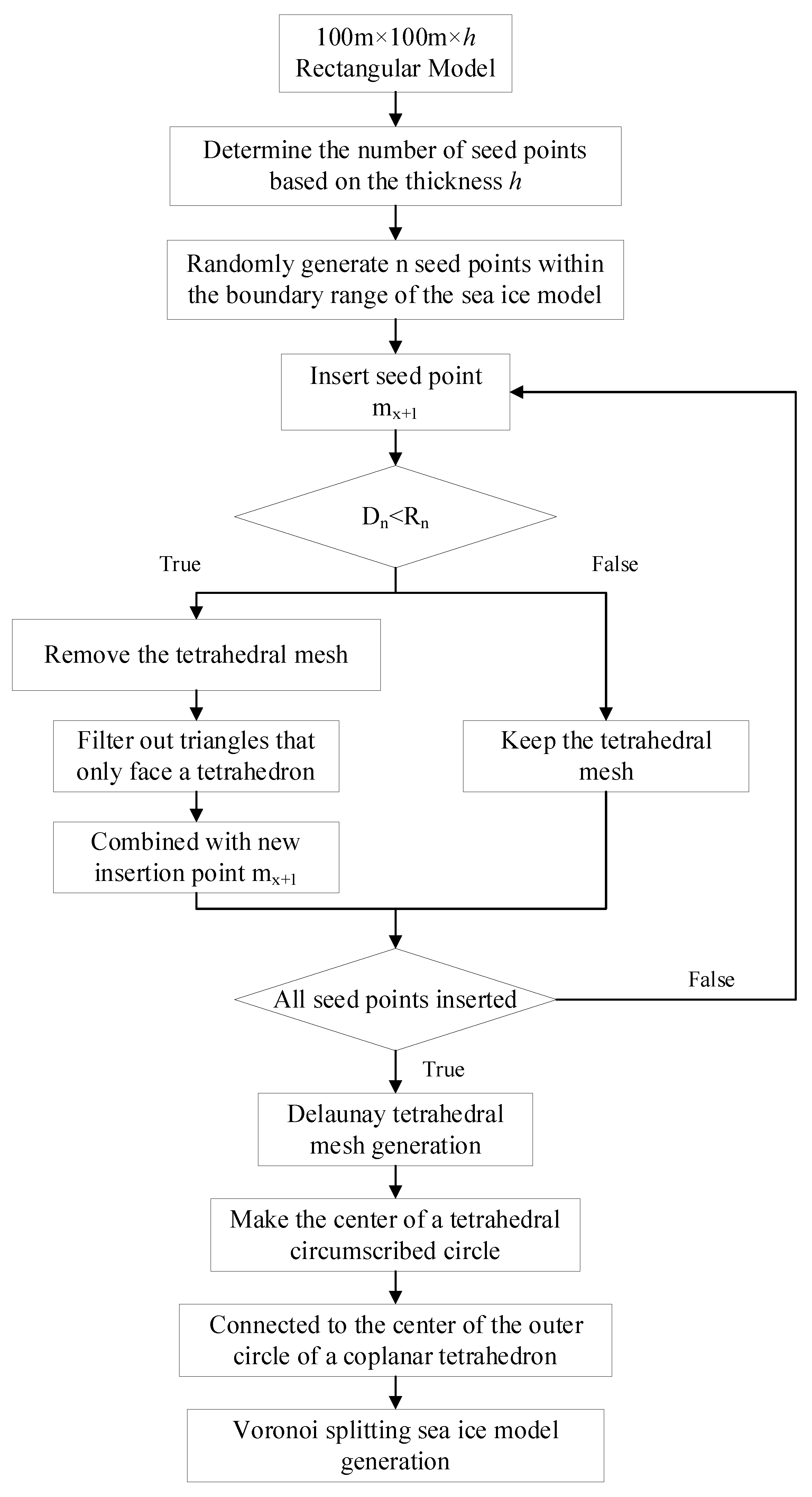
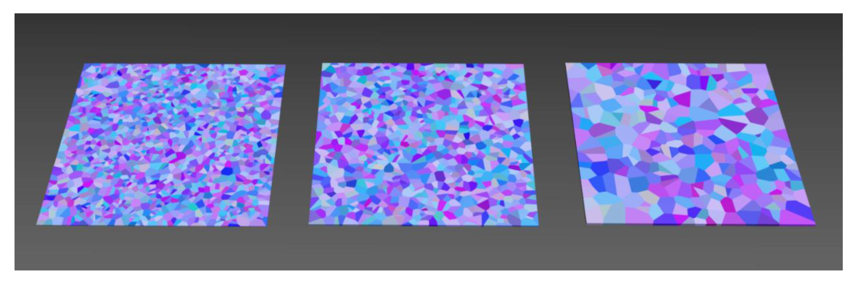
The Voronoi algorithm to was used preprocess a sea ice model, and the Voronoi algorithm was improved during processing so that the number of seed points was correlated with the thickness of the sea ice to determine the effects of different thicknesses on the degree of fragmentation.

(2)

Not only was the ship–ice interaction process used to generate the channel outline, but the ship’s movement on the sea ice around the channel also generated force conduction. In this study, the effect of conduction cracking on the ice surface near the channel was achieved.

(3)

After the sea ice broke up, there was no interaction between ice floes and seawater, i.e., there is no floating effect due to ice floes. After sea ice breaks up, the ice floe should be subject to the buoyancy of seawater, and this study incorporated the floating of the ice floe on the water surface by using a method based on the model grid.

(4)

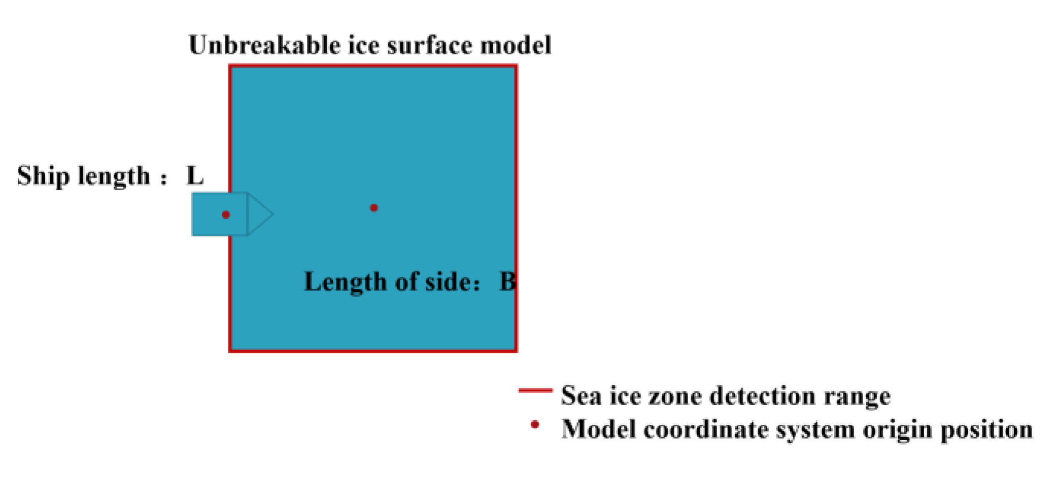
In terms of ice zone scene management, this study improved upon the quadtree scene management technique, used a circular detection area instead of a square detection area, and associated the detection area with the ship’s motion characteristics, leaving a certain amount of buffer for conduction cracking of the ice.

Compared with the approaches of other scholars, our method realized the effect of ice thickness on the size of broken ice, and the floating of broken ice is one of the features of this study. For various fractal algorithms, Voronoi algorithm is more suitable than Koch fractal algorithm with modeling ice breaking. Meanwhile, this study improved the Voronoi algorithm according to the relationship between ice breaking and ice thickness. Therefore, the fractal algorithm used in this study is superior to the traditional Voronoi and Koch fractal algorithms. Finally, by exploring the collision body arrangement method and improving the quadtree, the effect of conduction cracking on the ice surface near the navigation channel was realized, which ensures the real-time interaction of the navigation simulator. Thus, this study enhances the realism of the navigation scene in the ice area.

2. Methods

2.1. The Voronoi Diagram Algorithm for the Breaking up of Sea Ice Considering Ice Thickness

The effect of sea ice thickness on the degree of fragmentation is not considered in the preprocessing of existing sea ice models, and there are no scientific studies at home or abroad on the relationship between the number of fragments per unit area of ice and the ice thickness. In this study, the relationship between the number of fragments and the ice thickness was derived with a calculation based on the numerical algorithm implemented by Raed Lubbad et al. [5] for simulating ice zone navigation.

The numerical example implemented by Raed Lubbad et al. set the ice surface parameters, as shown in

Table 2. The input data for a large floating ice floe [5].

Ice thickness	1 m
Ice density	900 kg/m3
Ice modulus of elasticity	3 Gpa
Poisson’s ratio	0.33
Seawater density	1025 kg/m3
Acceleration of gravity	9.81 m/s2
The radius of the distributed load	0.5 m
The uniformly distributed vertical load	291 kPa
The flexural strength of the ice	500 kPa

.

The results of the algorithm are shown in

Table 3. The characteristics of the generated wedges [5].

Number of generated wedges	3	4	5
The angle of each wedge [deg]	60	45	36
The distance of the distributed load from the apex [m]	0.5	0.5	0.5
The maximum load capacity of each wedge [kN]	113	81	64
The breaking length [m]	4.5	4.5	4.5
The volume of each broken ice piece [m3]	11.7	8.4	6.6
The mass of each broken ice piece [tons]	10.5	7.5	5.9

, and the fragmentation pattern is shown in Figure 2. It can be deduced from the volume of a single piece of broken ice in Table 3 that when the ice’s thickness is 1 m and it is in the range of 100 m × 100 m, about 855–1515 fragments will be produced. At the same time, when the ice parameters are kept constant and the ice thickness is 0.5 m, the fracture length will be reduced from 4.5 m to 3.3 m [5], and from this, it can be deduced that when the ice’s thickness is 0.5 m and it is in the range of 100 m × 100 m, about 1165–2065 fragments will be produced. Among them, the fracture length will vary with the ice thickness, the elastic modulus of the ice, and the distance of the distributed load. It can be seen that the thicker the ice surface, the lower the number of fragments per unit area of the ice surface. In order to simulate this phenomenon, in this study, an algorithm that took ice thickness into account was designed to preprocess the sea ice model more scientifically.

Voronoi diagrams have a good fit of the fractal effect with the geometrical features of ice surface fragmentation [25], so we first dissected the ice surface into a Voronoi grid by using the 3D Voronoi diagram fractal algorithm. In order to correlate the fractal results with the ice thickness, in this study, a functional relationship between the number of seed points and the thickness of the ice model was constructed. This is performed as follows.

(1) In order to reflect the relationship between the ice thickness and the number and sizes of the fragments, the number of seed points generated has a certain quantitative relationship with the thickness of the ice model. In this study, we used the number of pieces of ice debris per unit area (100 m × 100 m) for an ice thicknesses of 1 m and 0.5 m, as deduced from the numerical example above, and we combined this with an interpolation method to calculate the number of pieces of debris generated per unit area for different ice thicknesses. This number is used to determine the number of seed points in the Voronoi diagram of the dissected ice surface model, as shown in the following equation:

$$\left\{\begin{array}{c}{n\left(h\right)}_{min}=[855+\frac{h-0.5}{1-0.5}\times \left(855-1165\right)]\\ {n\left(h\right)}_{max}=[1515+\frac{h-0.5}{1-0.5}\times \left(1515-2065\right)]\end{array}\right.$$

(1)

In the formula, ${n\left(h\right)}_{min}$ and ${n\left(h\right)}_{max}$ are the minimum and maximum values of the number of seed points generated, where [] represents the downward rounding of the calculation results, and the number of seed points is in the interval of [${n\left(h\right)}_{min}$, ${n\left(h\right)}_{max}$]; $h$ is the thickness of the ice model, and h is limited to the range of 0–1.5 m because this formula is deduced through interpolation, and the known data are the relationships between ice thicknesses of 0.5 m and 1.0 m and the quantity of fragments. However, the farther away from the known point of interpolation one is, the more inaccurate the calculation results may be, and at the same time, the ability of ships to navigate in an ice zone is also limited. Therefore, in this study, the range of values of $h$ is limited. The algorithm uses the known data for the interpolation to infer the number of seed points generated by the sea ice model for other thicknesses, i.e., the number of ice surface fragments generated by the algorithm.

(2) Using the generation of random coordinates, a total of n random coordinate points of m₁, m₂ … m_n are generated within the model boundary as seed points for the dissection, denoted as the set C(n).

(3) The tetrahedral mesh composed of the first x points (i.e., m₁, m₂ … m_x) in C(n) is denoted as T(x), and the Delaunay tetrahedral mesh is generated with the point-by-point insertion method by inserting the coordinate point m_x+1 and calculating the distance between m_x+1 and the center of the tetrahedral outer sphere in each T(x), D_n, and the corresponding radius R_n of the outer jointed ball. Following that, the tetrahedral lattices with D_n < R_n are filtered out and denoted as the set ET(x).

(4) The set ET(x) of tetrahedral meshes in which the outer jointed ball contains the insertion point m_x+1 is eliminated from the original tetrahedral mesh T(x), and a new tetrahedral mesh NT(x) is generated.

(5) Iterations are performed through all of the triangles in ET(x), and the triangles that face only one tetrahedron are filtered out and denoted as ∆(x).

(6) All of the triangles in ∆(x) are combined with the new insertion point m_x+1 to form a new tetrahedral mesh; this is added to NT(x) and reassigned to T(x).

(7) The above operation is repeated until all of the seed points are inserted, i.e., the final Delaunay tetrahedral mesh is obtained.

(8) Using the dyadic relationship between the Delaunay tetrahedral mesh and the Voronoi dissection result [33], the outer spherical center of each tetrahedron is connected to the outer spherical center of the coplanar tetrahedron to obtain the final dissection result.

The process of the above algorithm is shown in Figure 3.

In this study, sea ice was modeled using a rectangle as the original shape. Using the above algorithm, we dissected a 100 m × 100 m ice model with thicknesses of 0.2 m, 0.5 m, and 1.0 m, and the results obtained are shown in Figure 4 (the thickness increases from left to right), which shows the quantitative relationship between the number of fragments and the thickness of the ice surface, i.e., the thicker the ice surface is, the lower the number of sub-blocks per unit area dissected, and the greater the effect. In this way, we stored the processed model for use in laying down large-scale 3D scenes of the ice zone.

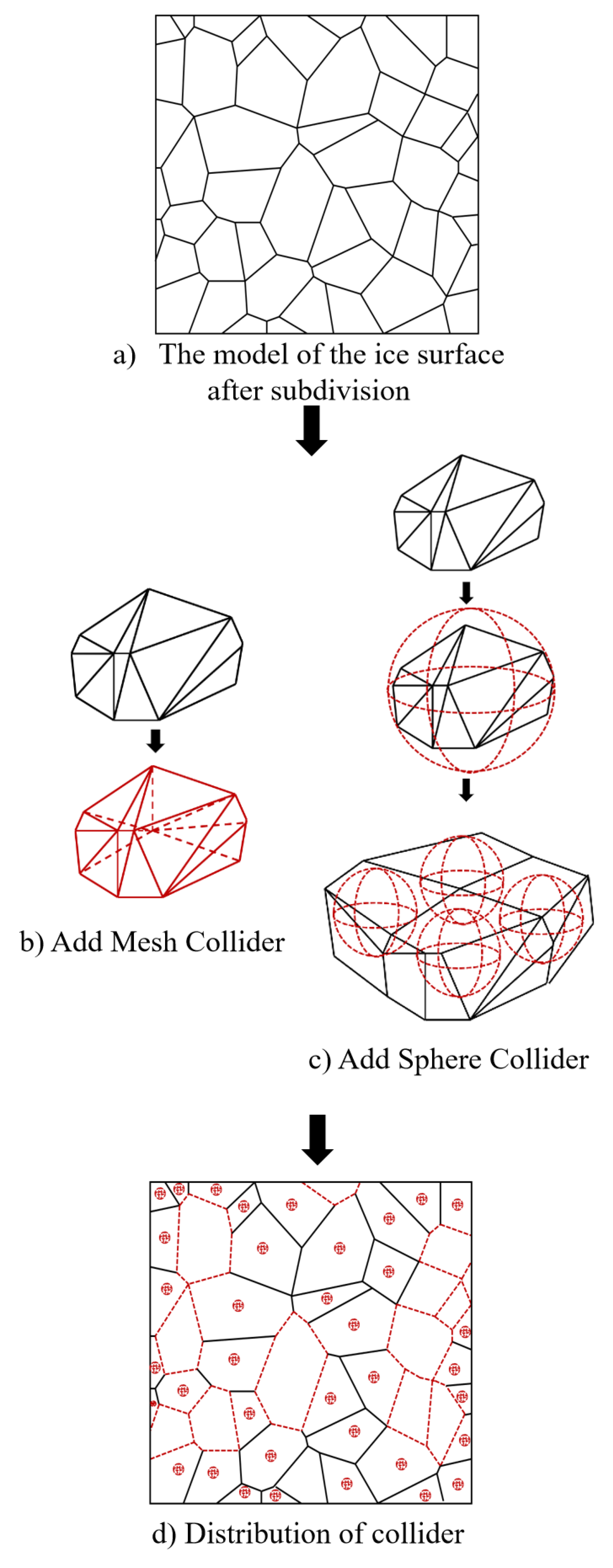
2.2. Collision Body Setup for Sea Ice Model Sub-Blocks

Using the above Voronoi diagram fractal algorithm, the cracking preprocessing of the sea ice model was realized by dissecting the sea ice model units into ice model sub-blocks, as shown in Figure 5a, which is a schematic diagram after the dissection. In order to simulate the fragmentation of the ice surface due to collision with a ship, it is also necessary to determine whether the ice model sub-blocks collide with the ship body.

Commonly used colliders include Box Collider, Mesh Collider, Capsule Collider, and Sphere Collider [34]. In order to fit the collision body with the ice model sub-blocks after the dissection of the Voronoi diagram algorithm, we initially chose the Mesh Collider. As shown in Figure 5b, the red line indicates the geometric boundary of the Mesh Collider.

Due to the good fit of Mesh Collider with the object geometry, in the case of a direct collision between some sub-blocks and the ship hull, all nearby sub-blocks will be displaced due to the contact, and the range of the conduction cracking will be too large, which is not in line with an actual situation. The use of Sphere Collider can inhibit the range of conduction cracking in ice to a certain extent; for this reason, this study combined the Mesh Collider and Sphere Collider to process the sea ice model, and the specific method is described in the following.

(1)

The Sphere Collider is added to a number of sub-blocks shown in Figure 5a, and the Mesh Collider is added to others.

(2)

There is a large redundancy with the sub-block geometry after adding the Sphere Collider enclosure, and there will be a large overlap between the collision bodies of the neighboring sub-blocks, so the radius of the Sphere Collider needs to be adjusted until there is no overlap between any of the Sphere Colliders, as shown in Figure 5c.

(3)

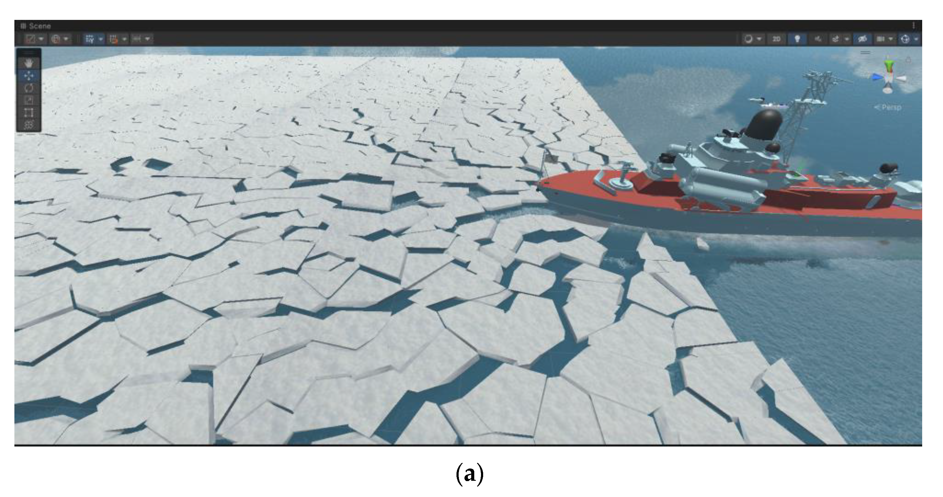
The distribution of collision bodies in the final ice model is shown in Figure 5d; the red dashed line indicates where the Mesh Collider was adopted to achieve a higher degree of fitting, while the Sphere Collider was adopted in other parts. This not only reproduces the effect cracking effect when a direct collision occurs, but this also optimizes the realism of conduction cracking.

(4)

The collision body information of the processed ice model sub-blocks is stored for calling when the large-area scene is laid out.

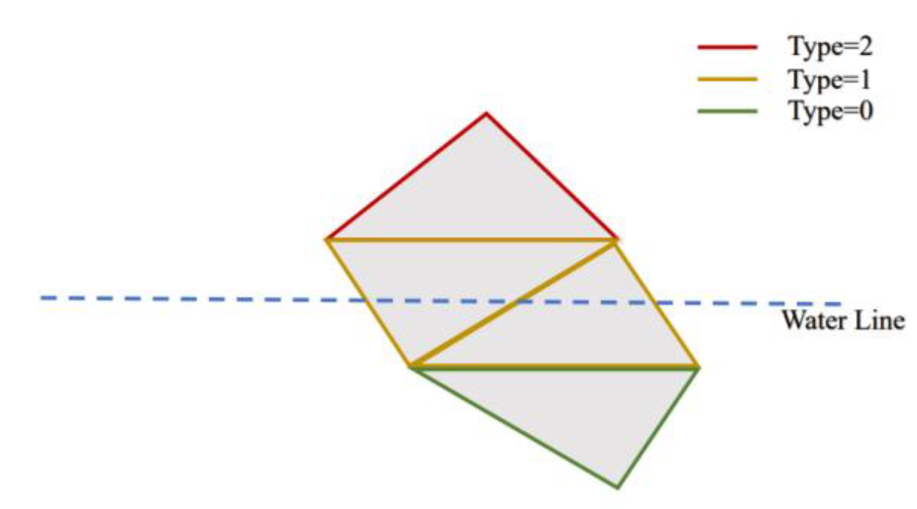
2.3. Simulation of the Floating State of the Ice Floes

The sea ice surface is broken under the action of collision with a ship, and the broken sea ice is subjected to the action of the seawater, causing drift, upward and downward movement, and other movement phenomena. As the Arctic ice zone is covered by a large area of ice, there are usually no large waves. This study assumed that the water surface on which the broken ice floes are located is calm, and only the floating of broken ice floes on the sea surface is simulated.

The sufficient and necessary condition for an ice floe to balance on the surface of water is that the combined force and moment are equal to zero, i.e., the buoyant force $R$ and the gravitational force G are equal in size and opposite in direction, and the lines of action coincide. From Archimedes’ principle, the buoyancy force equation is [35]:

$$R={\rho }_{\mathrm{s}}g{V}_{\mathrm{s}\mathrm{u}\mathrm{b}}$$

(2)

where $R$ is the buoyancy force; the seawater density ${\rho }_{\mathrm{s}}$ is set to 1.0270 g/cm³ [36]; the gravitational acceleration $g$ is set to 9.826 m/s² at sea level and 70° N [37]; the calculation of $V_{\mathrm{s}\mathrm{u}\mathrm{b}}$ makes use of the gridded data intercepted at the surface of the water in the model to derive the volume that should be underwater to satisfy

$${\rho }_{\mathrm{s}}g{V}_{\mathrm{s}\mathrm{u}\mathrm{b}}={-m}_{\mathrm{i}\mathrm{c}\mathrm{e}}g$$

(3)

The coupling of ice floes with seawater is realized with this equation. Here, $m_{\mathrm{i}\mathrm{c}\mathrm{e}}$ is the mass of the ice, and $g$ is the local gravitational acceleration.

In order to calculate the buoyancy by using the model mesh data and the relative position of the water surface, the vertex data and the triangular element index data of the mesh are first stored as the initial mesh data of the simulation object. When the simulation object interacts with the water surface, a part of the mesh enters below the water surface, and at this time, the triangular elements constituting the mesh appear in three cases, which are represented in this study by using integer data to refer to the type, as shown in Figure 6.

0: The triangular element is completely underwater.

1: The triangular element is partially underwater.

2: The triangular element is completely above the water.

After traversing the vertex data of all of the triangular elements in the mesh of this object, each triangular element has a corresponding type value. This value is used as a decision parameter for the next judgment of whether a triangular facet is cut by the water surface or not [38].

Next, the initial mesh of the object is intercepted, and the mesh of the part of the object below the water surface is intercepted in order to be used to calculate the drainage volume; all of the triangular elements in the simulation mesh of the object are traversed and are discarded if the type value is 2. If the type value is 0, the vertex data of the triangular elements are stored as mesh data intercepted from the water surface; if the Type value is 1, the situation needs to be further classified into the following two cases:

(1)

Two vertices are under the water.

(2)

One vertex is under the water.

When a triangular element has two vertices under the water surface, it needs to be dissected into two triangles, i.e., six vertices to be stored, as shown in Figure 7a; only one point under the water surface is sufficient for storing one triangle vertex, as shown in Figure 7b.

Following that, the volume of the seawater discharged by the object was calculated based on the water surface interception grid data, and the volume of the closure between the water surface and all of the triangular elements in the water surface interception grid data are accumulated, which results in the volume of the object’s drainage $V_{\mathrm{s}\mathrm{u}\mathrm{b}}$, and the sub-block that includes sea ice cracking reaches the equilibrium state on the sea surface when $V_{\mathrm{s}\mathrm{u}\mathrm{b}}$ satisfies Equation (3); thus, the floating of the ice floe is realized.

2.4. Scenario Management Based on the Improved Quadtree Algorithm

The sea ice field in a simulated ice zone scene usually needs to be laid out over a large area so that the view range is filled with sea ice models, but if all of them are dissected, sea ice models and each broken sub-block contain components such as rigid bodies, the Mesh Collider, and the Sphere Collider, which take up large amounts of computational resources, this will make it impossible to meet the real-time requirements for the view. Therefore, we need an efficient means of scene management.

In order to solve this problem, Sun Yuhao et al. proposed the use of the quadtree algorithm to manage the sea ice model, and they replaced the unbreakable model with a breakable model according to the location of the ship. However, since the sea ice model in this study achieves the effect of ice cracking conduction, it is not possible to replace the model strictly according to the ship’s location, and a certain amount of advancement is required. This study improves upon the basis of the traditional quadtree sea ice field management method.

The traditional quadtree detection method for sea ice fields involves detecting whether the ship’s position is within the sea ice model. However, because the ship model has a certain length, width, and height and the origin of the coordinate system is in the middle of the ship, when the ship’s hull enters a space of less than half of the ship’s length, the unbreakable ice model is not replaced with a breakable ice model. This would result in the ship’s hull being in contact with the ice surface without the ice surface being broken, making the realism of the ice zone scene poorer. This is shown in Figure 8.

To solve the above problems, this study uses 34 contour points to describe the ship’s hull, as shown in Figure 9. This enables the unbreakable model to be replaced by the breakable model in time to detect the collision so that the scene realism can be improved.

Since the arrangement of collision bodies adopted in this study allows the effect of ice conduction cracking to be achieved, the detection range of the sea ice field is changed from a square shape that perfectly fits the sea ice field to a circle in order to involve the sea ice in the vicinity of the ship’s position in the conduction effect. The center of the initial sea ice model is taken as the center of the circle, and half of the diagonal length of the ice model is taken as the radius to detect whether the ship’s position reaches the vicinity of the sea ice field. When the ship arrives near the edge, the model of the sea ice field is replaced by a breakable ice model, which acts as a buffer against cracking conduction in the sea ice field. In this study, the detection radius at this time is called $R_f$, and the detection area is called the fragmentation buffer, as shown in Figure 10.

Here,

$$R_f=\frac{\sqrt{2}}{2}B$$

(4)

$R_f$ is the radius of the fragmentation buffer and $B$ is the side length of the unbreakable ice model.

Due to the effect of the fragmentation buffer, the four corners of the model still fit closely to the edge of the detection area. Therefore, when the ship approaches the ice model from the corner, there will still be a situation in which the breaking of the ice cannot be detected in time. In order to solve this problem, the four corners should also be arranged with appropriate buffer areas. Therefore, in this study, 0.1 of the ship length is attached to the fragmentation buffer zone, and this is called the corner buffer zone; and the additional distance is denoted by $R_l$, as shown in Figure 11.

Here,

$$R_l=\frac{L}{10}$$

(5)

$R_l$ is the additional distance due to the corner buffer and $L$ is the ship length.

In summary, the radius of the detection range $R_T$ used in this study is

$$R_T=\frac{\sqrt{2}}{2}B+\frac{L}{10}$$

(6)

3. Experimental Results and Discussion

3.1. Experiments Comparing Different Ice Thicknesses

Since the degree of ice cracking and the sizes of broken ice floes are negatively correlated with the actual ice thickness in actual ice navigation processes, in this study, a three-dimensional navigation scene was simulated with different ice thicknesses in order to achieve this. The ice models were constructed with different thicknesses (as shown in Figure 4) and were arranged in the scene, and the results were observed and analyzed, as shown in Figure 12.

Figure 12a shows the condition of the channel edge and broken ice floes when the thickness was 0.2 m. The ice surface near the channel was more indirectly affected, generating a large number of broken ice floes and a wider channel width. When the sea ice thickness was 0.5 m, the channel width was narrower than when the thickness was 0.2 m. At the same time, due to the increase in thickness, the range of conduction cracking near the channel was smaller than the range of conduction breaking when the ice thickness was 0.2 m, so the width of the channel was slightly smaller than that in the case with an ice thickness of 0.2 m, which was in line with the laws of a realistic situation, as shown in Figure 12b. When the ice thickness was 1.0 m, due to the greater thickness, it was not easy for the nearby ice surface to be indirectly affected by the ship’s navigation, so there were no more obvious conduction cracking phenomena, as shown in Figure 12c.

In summary, the experimental results verified that dissecting the sea ice model after correlating the model thickness with the improved Voronoi diagram algorithm was able to improve the realism of the scene. However, the breaking of the ice was not only related to its thickness; there were many other key factors, such as the elastic modulus of the ice, the parameters of the ship model, and the relative speed of motion of the ship and ice. Therefore, the results of this experiment only reflect the possible influence of ice thickness on fragmentation. The influences of other factors on fragmentation will be further investigated in the future.

3.2. Experiments Comparing Different Collision Body Setups

In this study, three collider settings, namely, the Mesh Collider, Sphere Collider, and Mesh and Sphere Colliders, were used to process the model. The ice models processed with the three settings were arranged to lay out a wide range of ice in the three-dimensional scene for an experimental comparison and analysis.

The results of the experiment are shown in Figure 13. The first collision body setting is shown in Figure 13a. All of the sub-blocks in the sea ice model used the Mesh Collider, and it can be seen from the results that the ice conduction cracking achieved with this setting was not realistic enough. The ship only had to touch the edge of the scene to cause a wide range of cracking, which is unlike the results in a realistic situation.

The second collision body setting is shown in Figure 13b, where all of the sub-blocks in the sea ice model used the Sphere Collider. It can be seen from the results that, although this setting sacrificed some of the accuracy in collision detection, the shape of the channel edge that was produced was more realistic and more in line with an actual situation. However, the shortcoming of this method was that during the ship’s navigation process, although the ice surface near the channel did not directly collide with the ship’s hull, there was an indirect effect, making it undergo small-scale cracking and drifting. In other words, not only were irregularly shaped channel edges generated during navigation, but the ice surface near the channel was also affected and cracked, as Figure 14 shows. This kind of ice conduction cracking achieved by simply using the Sphere Collider’s collision body settings is not obvious enough, so we need to further optimize the collision body settings.

The final approach combined the Mesh Collider, which provided a better fit for the dissected geometry, and the Sphere Collider, which provided a slightly worse fit, for the sub-blocks in the sea ice surface model. The results of adopting this approach are shown in Figure 13c; both a more realistic shape of the channel edge and an indirect interaction with the nearby ice surface were produced, resulting in small-scale cracking and drifting phenomena, which further improved the realism and immersion of the scene. Understanding this from another perspective, the reason for why we chose to use the Sphere Collider in combination with the Mesh Collider and to sacrifice some of the accuracy in collision detection was that, in a real scenario, the ice surface at a distance is slightly deformed while the ship progresses, but not so much that it undergoes extensive fragmentation, as shown in Figure 13a. To ensure that this was accounted for, we chose to reduce the accuracy in collision detection, which is one of the drawbacks of the geometric approach to modeling in comparison with the physical approach to modeling. However, in order to balance realism and real-time performance, we still chose to use this method for the simulation in this study.

Meanwhile, the drawing efficiency was separately tested with the three collision body arrangements to achieve a 1000 m × 1000 m range with the computer hardware conditions: Intel(R) Core(TM) i5-7500 CPU 2.50 GHZ, 16 GB main memory, NVIDIA GeForce GTX 1650 GPU, and 8 GB graphic memory for the sea ice surface. The frame rate of the Mesh Collider method was 36.3 FPS, the frame rate of the Sphere Collider method was 61.3 FPS, and the frame rate of the Mesh and Sphere Collider method was 49.8 FPS, showing that the real-time performance of this study’s method was relatively moderate, and it is suitable for the large-scale depiction of an ice surface.

In summary, after adopting the Mesh and Sphere Collider setup proposed in this study, the sea ice model retained the advantages of the Mesh Collider and Sphere Collider for ice navigation scenes; this is a feasible collider setup that is more effective in enhancing the realism of a simulation of an ice navigation scene.

3.3. Floating Effect for Broken Ice Floes

Due to the irregular geometry of the ice model sub-blocks after dissection with the Voronoi algorithm, the normal vectors of the triangular elements in the sub-block mesh of the ice model were visualized in order to facilitate the observation of the angle between each triangular element and the water surface, as shown in Figure 15a. The green line segment represents the triangular grid below the water surface, and the red line segment represents the unit normal vector of each grid. When calculating the volume of an object below the water line, the cosine of the angle between the unit normal vector of the water surface and the normal vector of the triangular element was used so that the volume formed by the closure with the water surface corresponding to each of the triangular elements was directional. In the summation process, a volume corresponding to a triangular element at an obtuse angle with respect to the water surface was added as a positive value, and a volume corresponding to a triangular element at an acute angle with respect to the water surface was added as a negative value. In this way, the total volume of the object below the water surface could be found in order to achieve a floating effect, as shown in Figure 15b.

3.4. Improved Quadtree Scene Management

By using the cracking buffer and corner buffer proposed in this study, the problem of untimely model replacement when achieving cracking conduction was effectively solved, and the effect is shown in Figure 16. Figure 16a shows the fragmentation buffer with a detection radius of $R_T=\frac{\sqrt{2}}{2}B$, and Figure 16b shows the detection range of the ship after adding the corner buffer. The detection radius is a superimposition of the fragmentation and corner buffers, i.e., $R_T=\frac{\sqrt{2}}{2}B+\frac{L}{10}$.

The results before and after entering the detection area are shown in Figure 17.

A sea ice surface in the range of 6400 m × 6400 m was drawn under the computer hardware conditions of Intel(R) Core(TM) i5-7500 CPU 2.50 GHZ, 16 GB main memory, GPU NVIDIA GeForce GTX 1650, and 8 GB graphics card memory; the drawing frame rate was 98.2 FPS.

However, with the movement of the ship, the amount of the ice surface that will be breakable will become larger and larger, leading to a gradual decline in the frame rate at some viewpoints, which can be even lower than the minimum standards for real time, reaching the point of lag. Therefore, in the experimental process, the number of broken pieces and the frame rate of the relationship between samples of statistics at equal intervals in the scene were taken into account, and the ship maintained a uniform speed of straight-line movement, as shown in Figure 18. As can be seen in the figure, with the increase in the ship’s travel distance, the number of broken pieces grew. When the travel distance reached 400 m, the frame rate was lower than a smooth level, and when the travel distance reached 800 m, the frame rate was lower than the standard level. At this time, when the ship continued to move, the scene had lag, which decreased the sense of realism of the visual scene.

In order to solve this defect, the reverse of the quadtree detection algorithm was implemented. When the relative distance between the ship’s position and the breakable ice surface exceeded 700 m, the breakable ice models were destroyed and replaced by unbreakable ice models, which ensured that the number of fragments remained between 2800 and 3200 after the ship had travelled a certain distance. The frame rate remained above 30 FPS, which not only ensured a real-time navigation view in the ice zone but also made it possible to check the interaction of the ship with the ice at a certain distance. The experimental results are shown in Figure 19.

The experiments showed that the scene management algorithm used in this study made efficient use of computational resources while ensuring real-time and accurate scene interactions and improving the realism of the scene of an ice zone, as shown in Figure 20.

4. Conclusions and Outlook

This study improved the ice model preprocessing method and proposed to correlate the number of seed points in the Voronoi algorithm with the thickness of the ice model, so that the degree of fragmentation after the collision of the ice surface and the ship hull was differentiated in the simulation scene of traveling in the ice zone with different thicknesses of the ice surface, i.e., the effect of the thickness of the ice surface on the number of fragments and the size of the fragments was realized. This study explored the way of the collision detection of ship–ice collision. Mesh Collider and Sphere Collider were paired and used to set up the collision body for the ice model, and the ice breaking conduction effect realized using this model was more realistic, realizing the cracking and drifting of the nearby ice surface. At the same time, this study investigated the floating of broken ice. We calculated the volume size that a certain mass of broken ice should have below the waterline surface based on the positional relationship between the mesh triangular piece element and the water surface and Archimedes’ principle, allowing the floating of broken ice floes on the water surface to be realized. This study improved the ice area scene management algorithm. The traditional quadtree algorithm was improved to leave a sufficient buffer area for the interaction of ship ice, which improved the realism of the scene and meets the real-time requirements. These key technologies of ice area navigation scene simulation were improved, and the realism and immersion of the simulation scene was enhanced.

In future research, the correlation of the degree of sea ice breaking with the relative ship–ice impact speed should be considered. For the effect of floating ice floes, the torque generated by a non-collinear line of force should be considered, and three-degree-of-freedom rotation of ice floes can be simulated. At the same time, simulation processes should further consider the influence of the ship–ice interaction on the six-degree-of-freedom movement of the ship so as to further enhance the realism of ice zone navigation simulations. The realism of such simulations can be further improved.

References

1. Li, H.; Wang, S.; Wang, J.; Yu, L. Development Strategy for Polar Equipment in China. Chin. J. Eng. Sci. 2020, 22, 84–93. [Google Scholar] [CrossRef]
2. Information Office of the State Council. China’s Arctic Policy White Paper. Available online: http://www.scio.gov.cn/gxzt/dtzt/2018/zgdbjzcbps/bps_21653/202209/t20220921_430462.html (accessed on 27 April 2023).
3. China MSA. The Manila Amendments to the International Convention on Standards of Training, Certification and Watchkeeping for Seafarers, 1978; Dalian Maritime University Press: Dalian, China, 2010. [Google Scholar]
4. Admiral Makarov State University of Maritime and Inland Shipping. Introduction to Navigation Simulator in Ice Zone. Available online: https://prof.gumrf.ru/makarovka-stala-operatorom-krupnejshego-ledovogo-uchebnogo-tsentra-v-mire/ (accessed on 27 April 2023).
5. Lubbad, R.; Løset, S. A numerical model for real-time simulation of ship–ice interaction. Cold Reg. Sci. Technol. 2011, 65, 111–127. [Google Scholar] [CrossRef]
6. Norton, A.; Turk, G.; Bacon, B.; Gerth, J.; Sweeney, P. Animation of fracture by physical modeling. Vis. Comput. 1991, 7, 210–219. [Google Scholar] [CrossRef]
7. O’brien, J.F.; Hodgins, J.K. Graphical modeling and animation of brittle fracture. In Proceedings of the 26th Annual Conference on Computer Graphics and Interactive Techniques, Los Angeles, CA, USA, 8–13 August 1999; pp. 137–146. [Google Scholar] [CrossRef]
8. Pauly, M.; Keiser, R.; Adams, B.; Dutré, P.; Gross, M.; Guibas, L.J. Meshless animation of fracturing solids. ACM Trans. Graph. 2005, 24, 957–964. [Google Scholar] [CrossRef] [PubMed]
9. Steinemann, D.; Otaduy, M.A.; Gross, M. Fast arbitrary splitting of deforming objects. In Proceedings of the 2006 ACM SIGGRAPH/Eurographics Symposium on Computer Animation, Vienna, Austria, 2–4 September 2006; pp. 63–72. [Google Scholar]
10. Gingold, Y.; Secord, A.; Han, J.Y.; Grinspun, E.; Zorin, D. A discrete model for inelastic deformation of thin shells. In Proceedings of the ACM SIGGRAPH/Eurographics Symposium on Computer Animation, Grenoble, France, 27–29 August 2004. [Google Scholar]
11. Busaryev, O.; Dey, T.K.; Wang, H. Adaptive fracture simulation of multi-layered thin plates. ACM Trans. Graph. 2013, 32, 52. [Google Scholar] [CrossRef]
12. Pfaff, T.; Narain, R.; De Joya, J.M.; O’Brien, J.F. Adaptive tearing and cracking of thin sheets. ACM Trans. Graph. 2014, 33, 110. [Google Scholar] [CrossRef]
13. Stomakhin, A.; Schroeder, C.; Jiang, C.; Chai, L.; Teran, J.; Selle, A. Augmented MPM for phase-change and varied materials. ACM Trans. Graph. 2014, 33, 138. [Google Scholar] [CrossRef]
14. Tampubolon, A.P.; Gast, T.; Klár, G.; Fu, C.; Teran, J.; Jiang, C.; Museth, K. Multi-species simulation of porous sand and water mixtures. ACM Trans. Graph. 2017, 36, 105. [Google Scholar] [CrossRef]
15. Hu, Y.; Fang, Y.; Ge, Z.; Qu, Z.; Zhu, Y.; Pradhana, A.; Jiang, C. A moving least squares material point method with displacement discontinuity and two-way rigid body coupling. ACM Trans. Graph. 2018, 37, 150. [Google Scholar] [CrossRef]
16. Fan, L.; Chitalu, F.M.; Komura, T. Simulating Brittle Fracture with Material Points. ACM Trans. Graph. 2022, 41, 177. [Google Scholar] [CrossRef]
17. Iben, H.N.; O’Brien, J.F. Generating surface crack patterns. Graph. Models 2009, 71, 198–208. [Google Scholar] [CrossRef]
18. Glondu, L.; Muguercia, L.; Marchal, M.; Bosch, C.; Rushmeier, H.; Dumont, G.; Drettakis, G. Example-based Fractured Appearance. Comput. Graph. Forum 2012, 31, 1547–1556. [Google Scholar] [CrossRef]
19. Makarov, O.; Bekker, A.; Li, L. Comparative analysis of numerical methods for the modeling of ice-structure interaction problems. Contin. Mech. Thermodyn. 2022, 34, 1621–1639. [Google Scholar] [CrossRef]
20. Li, F.; Huang, L. A Review of Computational Simulation Methods for a Ship Advancing in Broken Ice. J. Mar. Sci. Eng. 2022, 10, 165. [Google Scholar] [CrossRef]
21. Dong, W.; Wang, Z. Simulation Study on Effects of Rigid Body Crushing. Comput. Knowl. Technol. 2021, 17, 5–6. [Google Scholar] [CrossRef]
22. Liu, N.; He, X.; Li, S.; Wang, G. Meshless simulation of brittle fracture. Comput. Animat. Virtual Worlds 2011, 22, 115–124. [Google Scholar] [CrossRef]
23. Zhao, F.; Zhou, M.; Geng, G. Fracture surface matching method of rigid blocks. J. Image Graph. 2017, 22, 86–95. [Google Scholar] [CrossRef]
24. Lyu, C.; Cao, L.; Huo, J.; Liu, X. Diversified Real-time Fracturing Simulation of Rigid Body. J. Image Graph. 2018, 23, 1403–1410. [Google Scholar] [CrossRef]
25. Sun, Y.; Yin, Y.; Pan, D. Rendering sea ice dynamic crushing in ice navigation scene based on Voronoi algorithm. Chin. J. Stereol. Image Anal. 2018, 23, 150–158. [Google Scholar] [CrossRef]
26. Fan, H. Research on Key Technologies of 3D Vision System for Ice Area Navigation Simulator; Jimei University: Xiamen, China, 2019. [Google Scholar]
27. Shao, X.; Zhang, X.; Yang, S.; Jin, Y. SPH fluid-solid interacted real-time solid fracture animation. J. Image Graph. 2023, 28, 2447–2460. [Google Scholar] [CrossRef]
28. Wu, X.; Lie, T.; Huang, G.; Wu, X. Research and Application of Complexity Scene Scheduling Strategy Based on Virtual Reality. J. Yangze Univ. (Nat. Sic Ed.) 2008, 5, 59–61. [Google Scholar]
29. He, R.; Shi, C.; Chang, W.; Wang, L. Application Research of Large-scale Terrain Dynamic Rendering Based on OSG. Comput. Digit. Eng. 2017, 45, 2022–2026. [Google Scholar] [CrossRef]
30. Chen, M. Optimized Scheduling Method Based on Maximum Flow Model for Complex City Scene Data; Southwest Jiaotong University: Chengdu, China, 2021. [Google Scholar]
31. Sun, Y.; Yin, Y.; Jin, Y.; Gao, S. Algorithm for Sea Ice Model Scene Management Based on Spatial Index. J. Syst. Simul. 2015, 27, 2427–2431. [Google Scholar] [CrossRef]
32. Sun, Y.; Yin, Y.; Gao, S. Research on Visualization of Ice Navigation in Marine Simulator. J. Syst. Simul. 2012, 24, 49–53. [Google Scholar] [CrossRef]
33. Zhou, P. Computational Geometry: Algorithm Design, Analysis and Application; Tsinghua University Press: Beijing, China, 2016. [Google Scholar]
34. Peng, X.; Ren, H.; Yu, J. Simulation training system of marine remote control grab. J. Dalian Marit. Univ. 2019, 45, 33–39. [Google Scholar] [CrossRef]
35. Jingyuan, W. Performance Analysis of Buoyancy Module of Marine Flexible Pipe System. Master’s Thesis, Dalian University of Technology, Dalian, China, 2021. [Google Scholar] [CrossRef]
36. Huang, L.; Wen, Y. Maritime Meteorology and Oceanography; Wuhan University of Technology Press: Wuhan, China, 2014. [Google Scholar]
37. Zhong, Z.; Luo, L. Handbook of Basic Physics; Guangxi People’s Publishing House: Nanning, China, 1983. [Google Scholar]
38. Zhang, J.; Ruan, C. A Triangle Rasterization Based on Improved Bresenham Algorithm. Electron. Meas. Technol. 2019, 42, 86–89. [Google Scholar] [CrossRef]
Figure 1. Comparison of the effects of simulating ice zone scenes: (a) effects achieved by Fan; (b) effects achieved by Sun with the Koch fractal algorithm; (c) effects achieved by Sun with the Voronoi algorithm; (d) effects achieved in this study.
Jmse 11 02047 g001
Figure 2. Fragmentation pattern [5].
Jmse 11 02047 g002
Figure 3. The process of the algorithm.
Jmse 11 02047 g003
Figure 4. Algorithm design process.
Jmse 11 02047 g004
Figure 5. Arrangement of the collider for the sub-blocks of the ice model.
Jmse 11 02047 g005
Figure 6. Types of triangular elements.
Jmse 11 02047 g006
Figure 7. Intercept mesh when type = 1: (a) two vertices under the water surface; (b) only one vertex under the water surface.
Jmse 11 02047 g007
Figure 8. Traditional quadtree scene management.
Jmse 11 02047 g008
Figure 9. Optimization using contour points.
Jmse 11 02047 g009
Figure 10. Fragmentation buffer zone.
Jmse 11 02047 g010
Figure 11. Corner buffer.
Jmse 11 02047 g011
Figure 12. Experimental results of models with different ice thicknesses: (a) h = 0.2 m; (b) h = 0.5 m; (c) h = 1.0 m.
Jmse 11 02047 g012aJmse 11 02047 g012b
Figure 13. Experimental results of the different model preprocessing methods: (a) Mesh Collider; (b) Sphere Collider; (c) Mesh and Sphere Colliders.
Jmse 11 02047 g013aJmse 11 02047 g013b
Figure 14. A realistic navigation scenario.
Jmse 11 02047 g014
Figure 15. Visualization of the unit normal vector of ice floes and the floating effect: (a) visualization of the unit normal vector; (b) floating effect.
Jmse 11 02047 g015
Figure 16. Schematic diagram of the detection radius (The red circles represent the boundary of the detection area.): (a) fragmentation buffer zone; (b) a superimposition of the fragmentation buffer and corner buffer.
Jmse 11 02047 g016
Figure 17. Schematic diagram of the detection radius: (a) before entering the detection area; (b) after entering the detection area.
Jmse 11 02047 g017
Figure 18. An increase in the ship’s travel distance leads to a decrease in the frame rate.
Jmse 11 02047 g018
Figure 19. The number of sub-blocks was controlled to maintain the frame rate.
Jmse 11 02047 g019
Figure 20. Improved quadtree scene management.
Jmse 11 02047 g020