Article

Optimization of Guide Vane Centrifugal Pumps Based on Response Surface Methodology and Study of Internal Flow Characteristics

1
Research Center of Fluid Machinery Engineering and Technology, Jiangsu University, Zhenjiang 212013, China
2
Wenling Fluid Machinery Technology Institute of Jiangsu University, Wenling 317500, China
*
Author to whom correspondence should be addressed.
J. Mar. Sci. Eng. 2023, 11(10), 1917; https://doi.org/10.3390/jmse11101917
Submission received: 19 September 2023 / Revised: 29 September 2023 / Accepted: 2 October 2023 / Published: 4 October 2023
(This article belongs to the Special Issue Advances in Marine Applications of Computational Fluid Dynamics)

Abstract

:
The methodologies of computational fluid dynamics (CFD) and response surface method (RSM) were integrated to uncover the optimal correlational framework for intricate hydraulic geometric parameters of guide vane centrifugal pumps. Parameters such as blade number, blade wrap angle, blade outlet angle, and relative axial distance between the guide vane and impeller, as well as radial distance, are embraced as optimization design variables. Meanwhile, pump head and efficiency were chosen as responsive variables. An analysis of 46 sets of hydraulic performance data was carried out by using the Box–Behnken experimental design method. Subsequently, response surface approximation models were established between hydraulic parameters and the efficiency, as well as the head. The optimal design point was predicted and a simulation of the hydraulic characteristics for the optimal scheme was conducted; the errors were 0.846% for head and 0.256% for efficiency between the simulation results with predicted results from RSM. The optimized model demonstrates noteworthy enhancements in hydraulic performance in comparison to the original model. By analyzing the internal flow of the optimized model under transient conditions, it was found that, as the internal flow of the flow passage components is relatively disordered at small flow rates, the amplitude of pressure pulsation is affected a lot. At other flow rates, the inside pressure pulsation waveform exhibits pronounced periodicity, and the primary causes of pressure pulsation in various flow components are not the same. Wall dissipation and turbulent dissipation emerge as significant contributors to the entropy generation in this centrifugal pump. The magnitude of entropy generation is correlated with the flow rate and the structural configuration of the pump’s components. High-entropy regions concentrate around the leading and trailing edges of the blades.

1. Introduction

A centrifugal pump is a hydraulic machine that generates centrifugal force using an impeller to convey liquids. It is widely used in various fields such as industry and agriculture. Centrifugal pumps have various classification methods based on different principles, structures, purposes, and transported media. The guide vane centrifugal pump is a common type of pump. Its main characteristic is that the velocity of the fluid transforms from axial to radial direction in the spatial guide vanes, the fluid can smoothly enter the downstream impeller or outlet pipe, and the hydraulic performance of the pump is enhanced because of vortices and eddies reducing. Guide vane centrifugal pumps are widely used in various fields such as urban water supply and drainage, industrial water supply, agricultural irrigation, energy, and the chemical industry.
To enhance the hydraulic performance of guide vane centrifugal pumps, scholars worldwide have conducted extensive research. Shi et al. [1] discovered that, in multistage deep well pumps, except at the first stage impeller inlet, circular flow existing at all other impeller inlets results in slightly lower head and efficiency. Zhou et al. [2] compared a cylindrical diffuser with a three-dimensional diffuser and found that the three-dimensional diffuser exhibits better overall hydraulic performance. Gong et al. [3] modified the wrap angle difference of the guide vanes to control the exit blade profile of the guide vanes, and found that the spatial guide vane exhibits better hydraulic performance when the wrap angle difference is positive. Liu et al. [4] conducted a study on the effects of different combinations of spatial guide vane inlet placement angles and inlet widths on submersible pumps. They found that a well-matched impeller and guide vane in submersible pumps could reduce hydraulic losses at the inlet of the guide vane. On the condition of depleted global resources and deteriorating environments, the significance of theoretical methods for optimizing pump design has grown; with the rapid advancements in computer technology and computational fluid dynamics (CFD) theory, researchers worldwide are combining design of experiment (DOE), surrogate model methods (SMMs), and intelligent optimization algorithms with CFD technology to optimize pump design. Kim et al. [5] employed DOE to optimize the design of a mixed-flow pump. They controlled changes in impeller shape by modifying impeller structural parameters, and successfully obtained a mixed-flow pump impeller that met the requirements. The variation trend of design variables with the specific speed was validated through numerical analysis and experiments. Heo et al. [6] conducted an optimization design of the inlet angle of mixed-flow pump guide vanes by using the SMM. The optimized model exhibited a significant improvement in efficiency at the specified specific speed. Safikhani et al. [7] applied a multiobjective genetic algorithm to Pareto optimization of centrifugal pumps and designed optimization methods for two conflicting target pump efficiencies and NPSH. This study employed RSM from the surrogate modeling method, which represented the system’s response as a function of one or more factors. This function relationship was displayed using graphical techniques, allowing for an intuitive identification of the optimization area. In recent years, the response surface method (RSM) has been progressively applied in the optimization of centrifugal pumps. Alawadhi Khaled et al. [8] conducted geometric optimization of a slurry pump by using the RSM and investigated the erosion and transient hydraulic characteristics of the optimized model. Wang et al. [9] optimized the guide vanes of a centrifugal pump by using the RSM and genetic algorithm, and revealed that the wrap angle of the guide vanes had the most significant impact on efficiency; the efficiency of the optimized model was improved by 8.65%. Kim et al. [10] conducted optimization of a centrifugal pump by using the CFD; the impeller was optimized by using RSM, while the volute was optimized by altering its cross-sectional distribution based on Stepanoff theory. As a result of these optimizations, the efficiency distributions of the impeller and volute were improved by 1.2% and 0.6%, respectively. M. Nataraj et al. [11] employed the RSM to optimize the geometric parameters of the impeller in a centrifugal pump, and the optimized impeller model exhibited an increase in head at the best efficiency point and a reduction of power consumption. Sushil Thakkar et al. [12] conducted an optimization design of a sanitary centrifugal pump by using RSM and multiobjective optimization methods. They improved the pump’s head and efficiency and investigated the impact of design variables on the head and efficiency. The abovementioned studies indicate that the combination of RSM and CFD technology is an effective method for centrifugal pump optimization. However, each researcher has carried out optimization designs for centrifugal pumps by using different variables based on their own considerations.
Centrifugal pumps operate in complex environments, and centrifugal pumps with guide vanes exhibit rapidly changing fluid velocities in the cavity region, resulting in unstable fluid flow within the pump. Consequently, the transient and unsteady features of the internal flow within guide vane centrifugal pumps have become more pronounced. Scholars from various regions have conducted extensive research on the transient flow characteristics and energy loss inside centrifugal pumps through numerical simulations and experimental validation. Wu et al. [13] summarized the fluid vibration characteristic by investigating the unsteady pressure pulsation and radial forces within the pump. They proposed optimization methods to reduce the vibrations and developed a predictive model for pump vibration. Posa and Lippolis [14] studied the influence of operating conditions and diffuser placement angle on unsteady flow and pressure pulsation in centrifugal pumps, and it was discovered that large flow rates and small radial clearances can both enhance the rotor–stator interference, leading to significant pressure pulsation. Shibata et al. [15] investigated the unsteady flow in multistage centrifugal pumps under off-design conditions. They found that the main cause of the positive slope phenomenon in the QH curve at low flow rates is the increase in diffuser losses.
Qi et al. [16] optimized centrifugal pumps by using the particle swarm optimization algorithm with the objectives of entropy production and efficiency. They found that the optimized pump’s entropy production was mainly attributed to wall dissipation and turbulence dissipation, concentrated around the leading and trailing edges of the blades. Majeed et al. [17] analyzed the unsteady flow field of a two-stage axially split centrifugal pump and used the entropy production term to evaluate turbulent kinetic energy dissipation to predict the loss locations for selective optimization in centrifugal pumps. Huang and Appiah et al. [18] investigated the entropy production mechanism within centrifugal pumps and found a strong correlation between pressure pulsation and the magnitude of entropy production. Appiah et al. [19] predicted the area and size of energy loss in fluid machinery by studying the entropy production rate in side channel pumps. Steffen Melzer et al. [20] derived a new entropy wall function for vane pumps, which reveals the relationship between local losses in specific flow regions and the efficiency characteristics of centrifugal pumps. The new entropy wall functions were applied to unsteady isothermal flow in a single-blade pump and to the partial load operation of traditional multiblade pumps. The study revealed how the local loss generation in specific flow regions influences the efficiency characteristics of centrifugal pumps. Yang et al. [21] investigated the clocking position of the inducer and impeller in high-speed centrifugal pumps. They found that the maximum efficiency difference between different phase positions was approximately 1.5%. The primary cause of this difference was identified as the turbulent dissipation within the impeller and diffuser.
This article takes a guide vane centrifugal pump as the object and designs 46 sets of experiments based on five design variables, which are blade number Z, blade wrap angle φ, blade outlet angle β2, axial distance ∆r, and radial distance ∆z between the guide vane and the impeller. This article uses multiple regression equations to fit the functional expression between design variables and response variables based on CFD simulation data, seeking optimal design points for various geometric parameters, and providing a reliable foundation for the optimization of the guide vane centrifugal pump by using RSM. Through the analysis of pressure distribution, streamlines, and entropy generation within the flow passage components, a deeper exploration is conducted into the fluid flow and energy losses within the pump.

2. Physical Model and Simulation Method

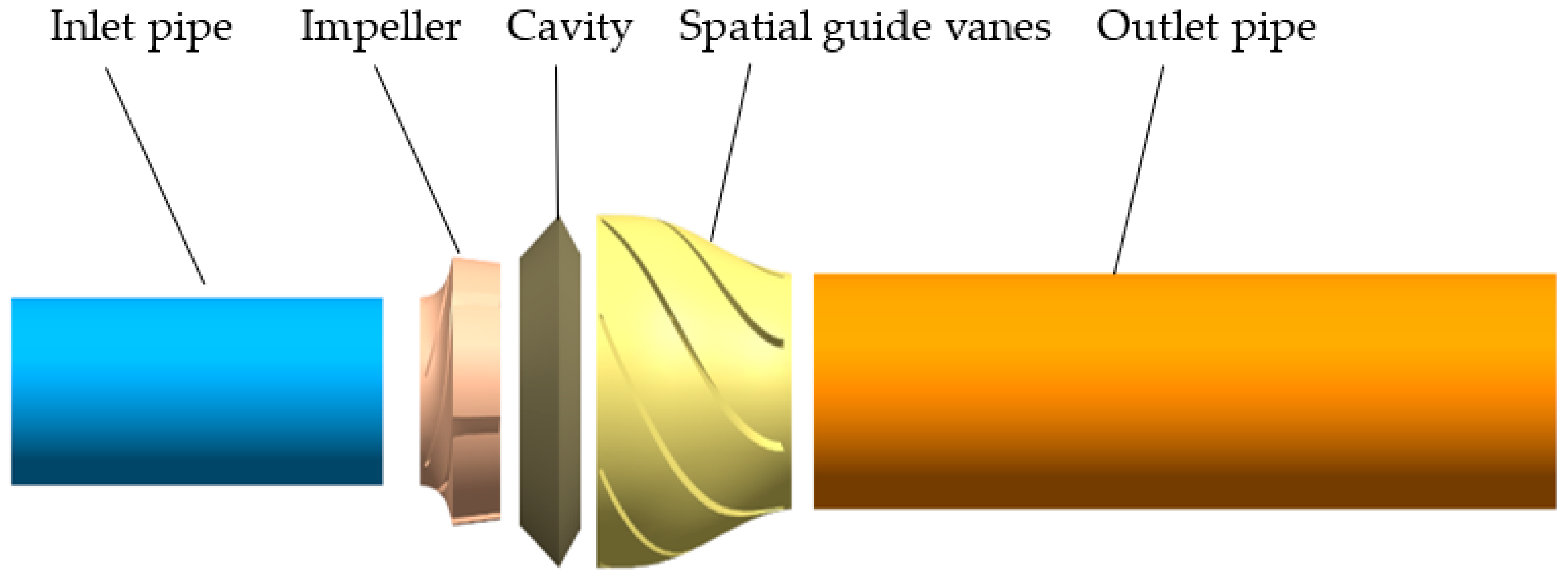
2.1. Structure and Basic Parameters

The research object of this article is a guide vane centrifugal pump driven by a submersible motor. The design head of the pump is Hd = 28 m, the design speed is n = 3000 r/min, and the specific speed is ns = 3.65nQ0.5/H0.75 = 55. The main components comprise a submersible motor, mechanical seals, an inlet chamber, a centrifugal impeller, and a spatial guide vane, as illustrated in Figure 1. Water is drawn into the impeller through the inlet chamber, undergoes centrifugal compression by the impeller, and is subsequently further rectified and pressurized by the spatial guide vane before being discharged.
Numerous structural parameters influence the performance of guide vane centrifugal pumps. Based on previous optimization studies on guide vane centrifugal pumps and the original pump model, this article selects five optimization design variables for experimental design: blade number(Z), blade wrap angle (φ1), blade outlet angle (β2), axial distance between the guide vane and the impeller (∆z), and the radial distance (∆r). The geometric features of the variables are illustrated in Figure 1 and Figure 2.
The primary hydraulic dimensions are presented in Table 1.

2.2. Numerical Simulation Configuration

This paper employs the ANSYS CFX19R3 software for numerical simulation. The entire flow field was set to a three-dimensional incompressible steady viscous turbulent flow field. The time-averaged continuity equation and momentum equation are established in a relative coordinate system, the turbulence model was set to the SST k-ω turbulence model, and a fully implicit coupled algorithm was used. The impeller is designated as the rotating domain with a rotational speed set to 3000 r/min, while the remaining simulation domains are defined as stationary. The inlet and outlet boundary conditions were set to total pressure inlet and bulk mass flow rate outlet, respectively. The interfaces between the rotor (impeller) and stators (inlet pipe and cavity) were set to “frozen rotor”, and interactions among other stators were “none”. The wall surface roughness was set at 0.03 mm, and the convergence criterion was set at 10−4. During unsteady simulations, the “frozen rotor” interface was replaced with the “Transient Rotor Stator”. To attain more stable and accurate data, a total time of 0.2 s, corresponding to 10 revolutions, was designated. The time step was set at 0.0001666 s (calculations performed every 3°).
The SST k-ω model combines the advantages of both the k-ε model and the k-ω model. The k-ε model is applied in regions outside the boundary layer, while the k-ω model is used within the boundary layer. The SST k-ω model demonstrates significant advantages in handling adverse pressure gradient flows and separated flows. A considerable portion of energy loss in guide vane centrifugal pumps originates from flow separation [22]. Therefore, the turbulence model chosen for this study is the SST k-ω turbulence model, and its transport equations are as follows:
( ρ k ) t + ρ u i k x i = P ˜ k β * ρ k ω + x i μ + σ k μ t k x i
( ρ ω ) t + ρ U i ω x i = α 1 v t P ˜ k β ρ ω 2 + x i μ + σ ω μ t ω x i + 2 1 F 1 ρ σ w 2 1 ω k x i ω x i
In the equation, kinematic eddy viscosity v t = a 1 k max a 1 ω , S F 1 , turbulent kinetic energy generated by eddy shear P ˜ k = min μ t u i x j u i x j + u j x i , 10 β * ρ k ω , and auxiliary function F 1 = tanh min max k β * ω y , 500 v y 2 ω , 4 ρ σ ω 2 k C D k ω y 2 , C D k w = max 2 ρ σ ω 2 1 ω k ω x i x i , 10 10 . Other empirical constants:  β * = 0.09 , α 1 = 5 9 , β 1 = 3 40 , σ k 1 = 0.85 , σ ω 1 = 0.5 , α 2 = 0.44 , σ k 2 = 1 , β 2 = 0.0828 , σ ω 2 = 0.856 .

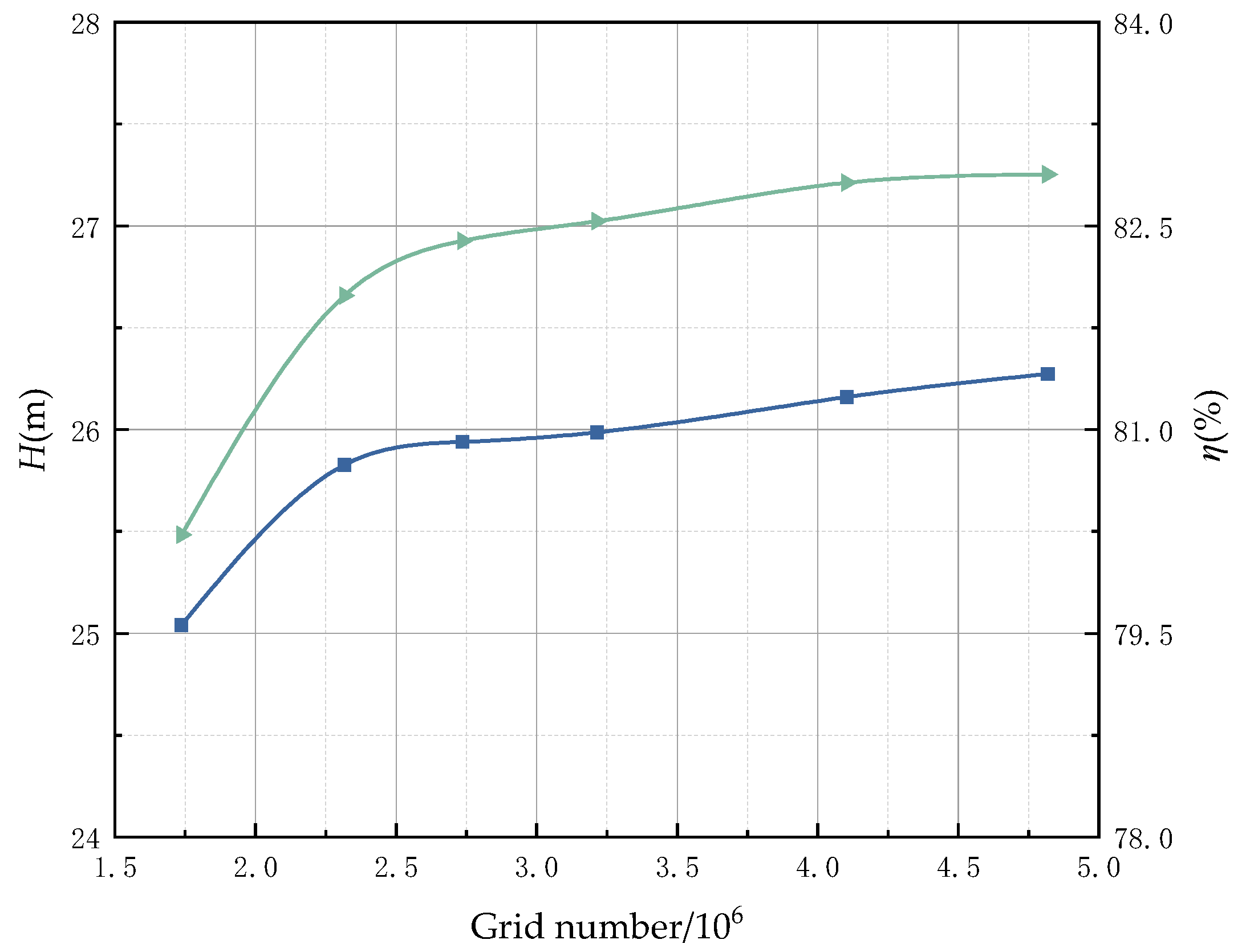
2.3. Simulation Domain and Mesh

The simulated domain is simplified as the combination of inlet pipe, impeller, cavity, spatial guide vane, and outlet pipe, as depicted in Figure 3. The length of the inlet pipe is 2.2 Dj, while the length of the outlet pipe is 4.4 Dj. Mesh generation is a crucial step in numerical simulations, where high-quality meshes enhance the accuracy of the simulation results and simulation efficiency. The meshing of the simulation domain is performed using the mesh generation tool ICEM19R3 and TurboGrid19R3 software. The structured hexahedral mesh is used in the whole simulation domain, and the boundary layer meshes are suitably refined, achieving a mesh quality higher than 0.31.
The simulation results can be influenced by grid numbers. The mesh independence was conducted using five different grid numbers, as shown in Figure 4. When the number of grids increased from 1.73 million to 4.1 million, the head showed an upward trend, with a very small increase of over 4.1 million. As the number of grids increases, the efficiency shows an upward trend and the amplitude becomes smaller and smaller. Considering the balance between computational accuracy and the computational load imposed by grid numbers, the total number of grids was about 4.10 million. The grid numbers for the inlet pipe, impeller, cavity, guide vanes, and outlet pipe were 222,912, 1,261,033, 107,823, 1,828,758, and 683,027, respectively. In this paper, most areas on the impeller blade surface and the guide vane blade surface have a Yplus value of 10 or less, while in a few regions, due to the complexity of the structure, the Yplus value is at a higher level.

3. Experimental Validation

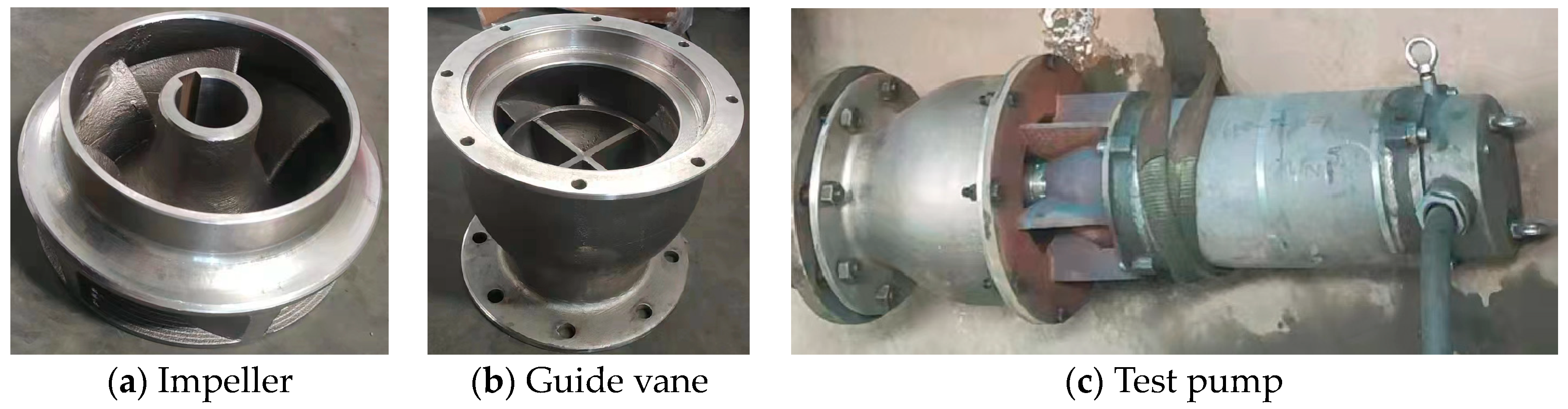
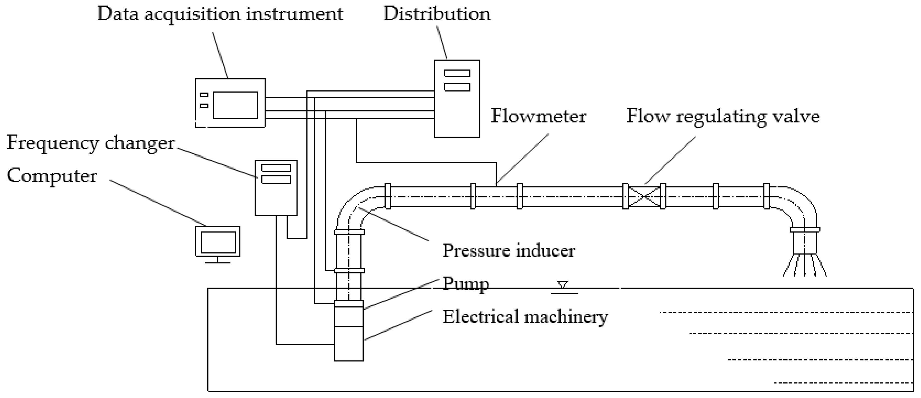
3.1. Experimental Equipment

To verify the accuracy of the numerical simulation results for the external characteristics of the guide vane centrifugal pump, experimental research on the external characteristics of the design model was conducted. The subject of the experiment was the WQ200-28-22 guide vane centrifugal pump, with the designed flow of Qd = 200 m3/h, the designed head of Hd = 28 m, and the speed n = 3000 r/min. The experimental model is illustrated in Figure 5. The experimental platform primarily consists of a guide vane centrifugal pump, a frequency converter, an outlet pipeline, an outlet control valve, an outlet pressure sensor, a flowmeter, and a data acquisition instrument, as shown in Figure 6. The driving system employs a high-speed permanent magnet motor, and the speed of centrifugal pump is regulated by the frequency converter. The flow rate is adjusted through valves on the pipeline, and the outlet pressure of the centrifugal pump is monitored by using a pressure sensor. The outlet pipeline has a diameter of 150 mm. The WT2000 pressure sensor is employed with a measurement range of 0~1.6 MPa and a comprehensive accuracy of ±0.5%. The flowmeter utilized is the LWGY-150A0A3T model turbine flowmeter with a testing accuracy of ±0.5%. The data acquisition instrument uses a TPA-3A hydraulic machinery comprehensive testing instrument.

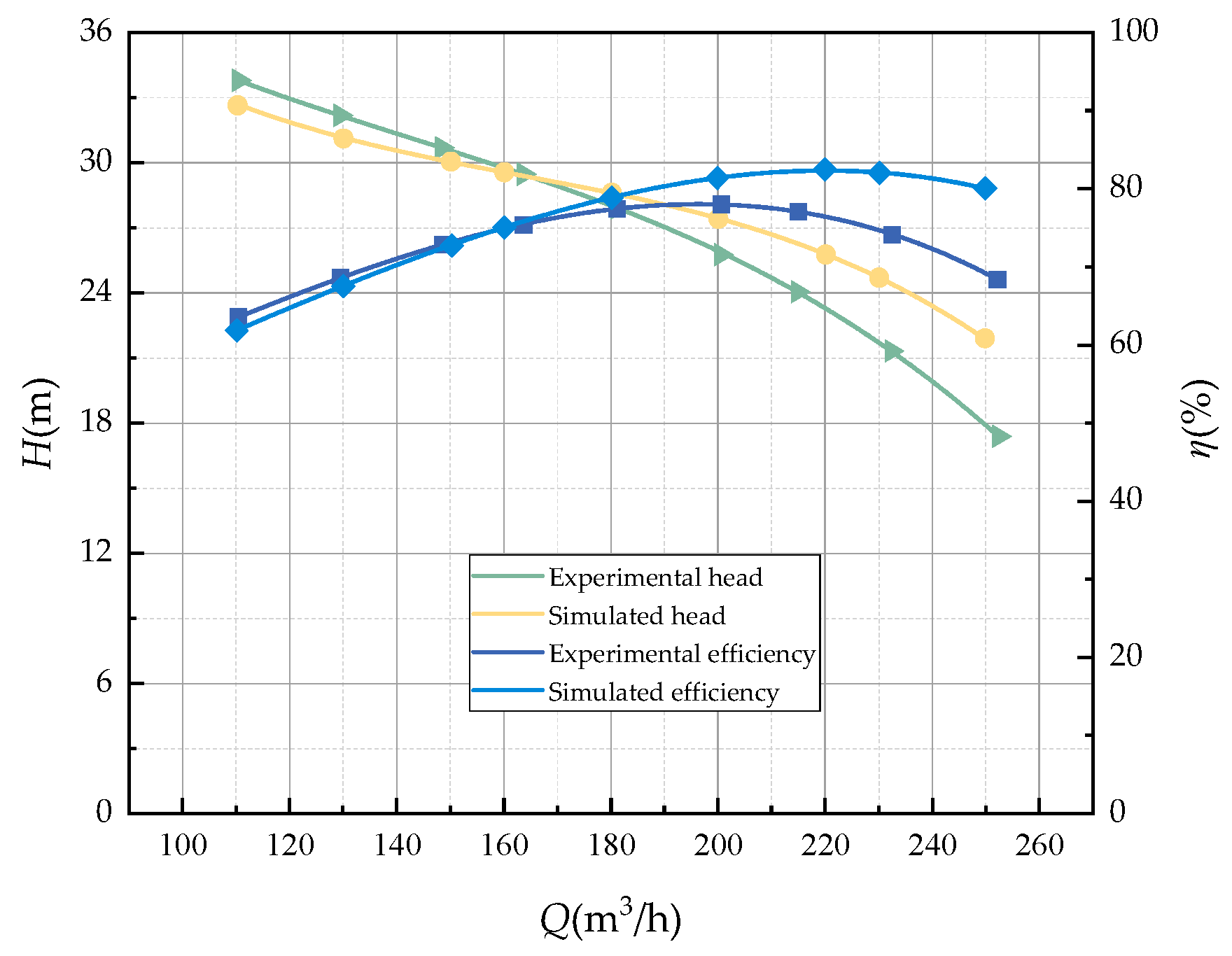
3.2. External Characteristic Test Results

Figure 7 shows the comparison between the experimental data and the simulation data of the centrifugal pump under different flow rates. The trends in the experimental and simulated data shown in the figure are closely aligned. At small flow rates, the experimental data and simulated data in the figure exhibit a similar trend, and the error is very small. As the flow rate exceeds 160 m3/h, the error gradually increases, with simulated values slightly higher than experimental values. At rated flow rate, the head error is approximately 1.24 m, and the efficiency error is around 3.2%. These errors fall within an acceptable range, indicating the reliability of the numerical simulation approach employed in this study. The main causes of errors are as follows: (1) The model used in the numerical simulation has been simplified, especially for the inlet pipe section; it is simplified from spatial inflow to a vertically entering pipe. As the flow rate increases, hydraulic losses at the spatial inflow location in the experimental model also intensify, contributing to an increase in error between the simulated and experimental values. (2) During numerical simulation, the omission of the impeller inlet’s ring gap results in a simulated outcome that tends to be higher compared to the actual conditions. (3) Disparities between the cast components of the impeller and guide vanes and the designed model impact the hydraulic performance of the experimental pump.

4. Response Surface Optimization Analysis

4.1. Mathematical Model

The majority of RSMs utilize second-order response surfaces, with their earliest application introduced by Box and Wilson [23]. A surface is formed in space by two variables, and the equation describing the surface is as follows:
Y = a 1 + 1 n a i x i + 1 n a i 2 x i 2 + 1 n a i j x i x j
In the equation, a 1 , a i , a i 2 , and a i j are coefficients; x i and x i 2 represent the first and second order terms of the response variables, respectively; x i x j stands for the interaction term of the response variables.
Variance is employed to express the degree of dispersion between a random variable and its expected value. The mathematical expression is as follows:
S 2 = x 1 x ¯ 2 + x 2 x ¯ 2 + + x n x ¯ 2 / n
In the equation, S 2 represents variance; x 1 , x 2 , ……, x n are random variables.

4.2. Response Surface Experimental Design and Results

Table 2 presents the factor levels of the five design variables (blade number Z (A), blade wrap angle φ1 (B), blade outlet angle β2 (C), radial distance between guide vane and impeller ∆z (D), and axial distance between guide vane and impeller ∆r (E)). Using the pump head H and efficiency η as response variables, the experimental design was carried out by using the Box–Behnken design method in the Design Expert12 software. The experimental design resulted in 46 sets of schemes, which were analyzed by using the simulation method mentioned earlier. The results are shown in Table 3.

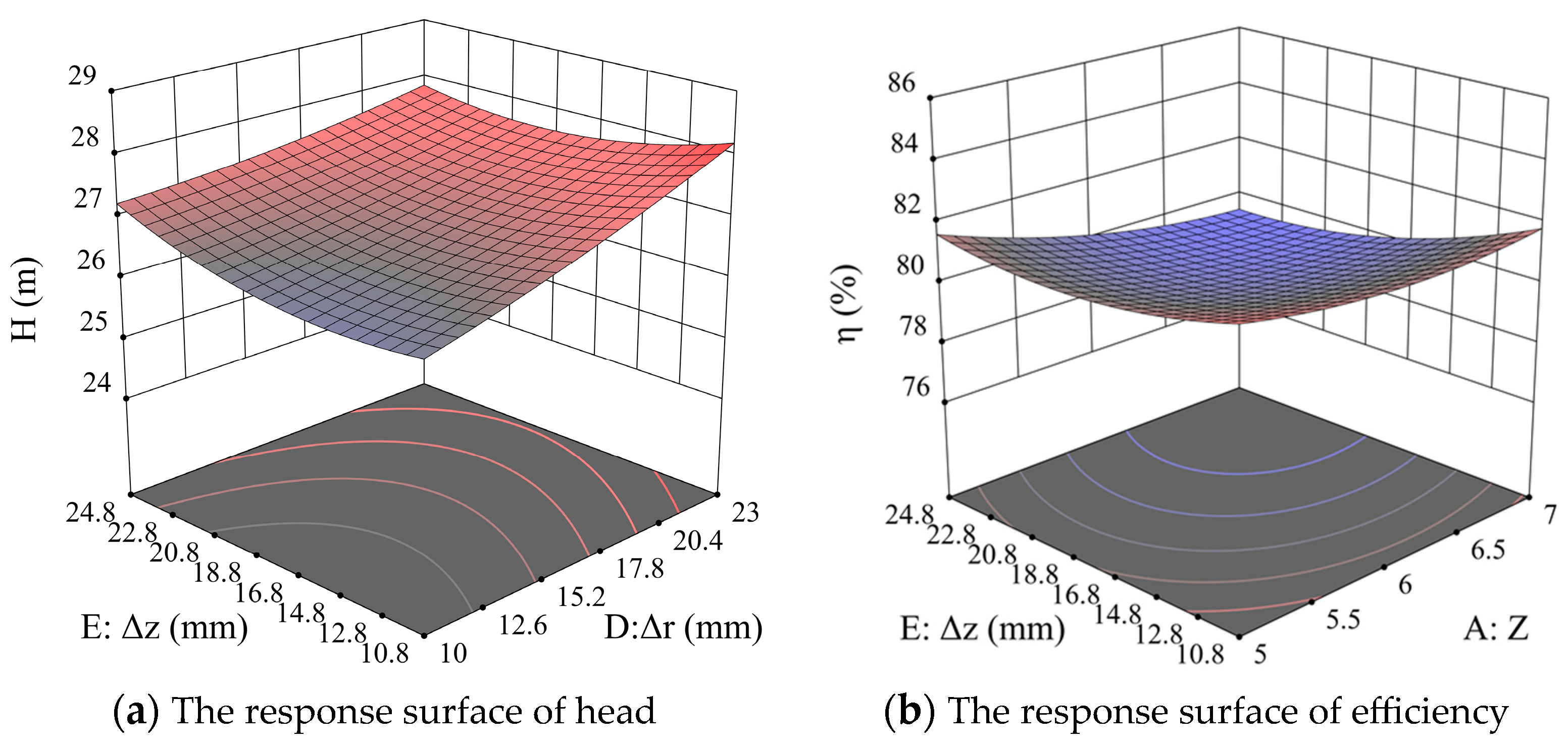
4.3. Model Fitting and Response Surface Analysis

Response surface analysis often employs second-order polynomials. The equation is provided in the previous response surface mathematical model. This article uses second-order polynomials to fit the functional relationship between design variables and response variables as follows:
H = + X 1 + X 2 A + X 3 B + X 4 C + X 5 D + X 6 E + X 7 A B + X 8 A C + X 9 A D + X 10 A E + X 11 B C + X 12 B D + X 13 B E + X 14 C D + X 15 C E + X 16 D E + X 17 A 2 + X 18 B 2 + X 19 C 2 + X 20 D 2 + X 21 E 2
η = + Y 1 + Y 2 A + Y 3 B + Y 4 C + Y 5 D + Y 6 E + Y 7 A B + Y 8 A C + Y 9 A D + Y 10 A E - Y 11 B C + Y 12 B D + Y 13 B E + Y 14 C D + Y 15 C E + Y 16 D E + Y 17 A 2 + Y 18 B 2 + Y 19 C 2 + Y 20 D 2 + Y 21 E 2
where Xi and Yi are coefficients, and their specific values can be found in Table 4.
To assess the fitting degree and predictive accuracy of the model, the model’s p-value, as well as the coefficient of determination (R²), adjusted coefficient of determination ( R a d j 2 ), and predictive coefficient of determination ( R p r e 2 ), were analyzed to validate the model. The p-value is used to test the significance of each parameter in the model. When the p-value is less than the predetermined significance level (typically set at 0.05), it indicates that the factor has a significant impact on the model. R² and R a d j 2 are measures of the fitting accuracy of the regression equation [24], with values ranging between 0 and 1. Their values closer to 1 indicate that the model fits the data better. R p r e 2 is an indicator used to assess the predictive ability of the model. Generally, a difference within 0.2 between R a d j 2 and R p r e 2 indicates that the model has good predictive performance. The results of the variance analysis of the model’s regression equations are presented in Table 5. The p-value for each response variable is less than 0.0001, indicating the model’s high significance. The R a d j 2 values for head and efficiency are 0.9658 and 0.8318, respectively, indicating a good fit of the regression equations. The difference between R p r e 2 and R a d j 2 for head and efficiency is 0.0352 and 0.0674, respectively. This signifies a relatively high accuracy of fitting, indicating that the model can predict the internal performance of the centrifugal pump quite well. Figure 8 illustrates a comparison between the actual and predicted values of head and efficiency. The X-axis represents the actual values of the design points, while the Y-axis represents the simulated values of the design points. Blue represents low levels, while red represents high levels. Most of the design points in the graph are situated around the line of equality (X = Y), indicating that the accuracy of predictions has been ensured.

4.4. Analysis of Factor Significance

The hydraulic parameters of a centrifugal pump interact and influence each other, and there are rarely completely independent relationships among structural parameters. The interaction between structural parameters may have a significant impact on the response variables of this design. Therefore, when analyzing factor significance, both single-factor and two-factor effects should be simultaneously considered. Table 6 and Table 7 present the influence of each factor on head and efficiency. It can be observed from the tables that all five single-factor terms have a significant impact on both head and efficiency. In terms of the single-factor quadratic terms, Z2, β22, and φ12 have a highly significant impact on head; β22, φ12, and ∆z2 have a highly significant impact on efficiency. In terms of factor interactions, the ∆r∆z term has the most significant impact on head, while the Z∆z term has the most pronounced influence on efficiency. Figure 9a depicts the response surface plot illustrating the influence of ∆r∆z on the head. When ∆r is 10 mm, with the increase of ∆z, H shows an upward trend in a U-shaped curve. When ∆r is set to 23 mm, with the increase of ∆z, H demonstrates a downward trend in a U-shaped curve. This variation indicates a significant interaction between ∆z and ∆r. Figure 9b depicts the response surface plot illustrating the influence of Z∆z on the efficiency. When ∆z is at a low level, the variation of Z has little influence on η. However, when ∆z is at a high level, η shows a decreasing trend with the increase of Z. This variation indicates an interaction between Z and ∆z. When Z and ∆z take their minimum values, η reaches its maximum value.
In summary, the single factors and their quadratic terms of the design factors have a significant impact on the response variables. There are interactions between factors, but compared to the single factor and single factor quadratic terms, the interaction effects are relatively weaker.

4.5. Analysis of Optimization Results

The numerical optimization algorithm in Design12.0 can assign weights to each objective to adjust the shape of its particular desirability function. The weight ratio of head and efficiency in this article is set at 4:5. When combining Equations (5) and (6) along with the factor levels of the design factors, the optimal parameter combination is determined to be Z = 7, β2 = 23.8°, φ1 = 100.7°, ∆r = 22.814 mm, and ∆z = 13.838 mm. Numerical simulations were performed in CFX for the optimal parameter combination, and a comparison was made with the simulation values of the original model. Table 8 presents the predicted and simulation values of the pump head and efficiency before and after model optimization. The simulation values of the original model were selected from the intermediate dataset in Table 4. From the data in Table 8, it can be observed that the simulation values and predicted values of the model are in good agreement, indicating the reliability and accuracy of using the RSM for the optimization of the guide vane centrifugal pump. The optimized model shows improvements in hydraulic performance compared to the original model, with an increase of 2.5845 m in head and 2.88% in efficiency, respectively. The increase in head is within ±7% of the rated head of 28 m, and the efficiency still improves by around 3% when it is above 80%. The optimization effect achieved the expected outcome.
To better observe the variation of head in the entire flow process of the original and optimized models, the spatial Z-axis values are taken as the X-axis and the head coefficient Ha as the Y-axis in a two-dimensional plot. Head coefficient H a = P ave P inlet / ρ g , where Pinlet represents the average pressure at the inlet surface (Pa), and Pave refers to the average pressure at any cross section of the guide vane centrifugal pump (Pa).
Figure 10 shows the variation curve of head coefficient along the Z-axis at flow rates of 0.6Qd, 1.0Qd, and 1.4Qd. In the figure, the original model is denoted as M1, while the optimized model is labeled as M2. As depicted in Figure 10, it is evident that, compared to the original model, the optimized model exhibits larger absolute values of Ha at the inlet of the impeller to the inlet of the blades at various flow rates. This suggests an improved suction capability of the optimized model in this specific region. At both rated and large flow rates, the optimized model displays a more rapid increase in Ha, particularly within the cavity region. The difference between the Ha values of the optimized and original models further widens, indicating that the optimization of ∆r and ∆z has modified the shape of the cavity, resulting in an improved flow state of the fluid within the cavity. As a static component, the internal flow state of the guide vane is primarily influenced by the fluid flow within the cavity. Therefore, the internal fluid flow state of the optimized model guide vane is more stable, and the Ha descent speed is smaller. At small flow rates, the internal fluid flow within the guide vane centrifugal pump tends to be turbulent. Both before and after model optimization, the trend of Ha variation near the impeller remains consistent, with similar numerical values. At the inlet of the guide vane, both models showed a sharp increase and decrease in Ha, and in the guide vane and outlet pipe, the decrease in Ha of the original model was greater than that of the optimized model. This indicates that the fluid flow at the inlet of the guide vane in the original model is more turbulent, which further affects the fluid in the guide vane and outlet pipe sections.

5. Internal Flow Characteristics of the Guide Vane Centrifugal Pump

5.1. Pressure Distribution and Streamlines

Figure 11 shows the pressure distribution and streamlines on the central plane of the main flow components for the guide vane centrifugal pump at three flow rates: 0.6Qd, 1.0Qd, and 1.4Qd. Overall, from the inlet of the impeller to the outlet of the guide vane, the pressure value of the centrifugal pump increases from low to high, and slightly decreases at the outlet of the guide vane. With the increase in flow rate, the fluid flow rate within the flow components rises, resulting in a decrease in pressure values and pressure gradients on the central plane. In addition, Figure 11c reveals that there is a localized low-pressure region near the leading edge of the blade working surface at large flow rates (indicated by the red dashed line in the figure). This indicates that at large flow rates, the flow velocity increases significantly near the leading edge of the blade, accompanied by abrupt changes in flow direction. This leads to the formation of a flow separation region at the leading edge of the blade, where the fluid detaches from the blade surface, resulting in a localized low-pressure area.
In terms of streamline, Figure 11b,c show that the flow pattern of the fluid inside the impeller and cavity is good at rated and large flow rates, with small vortices appearing at the inlet of the guide vane. But the notable vortex appears near the outlet of the guide vane; this indicates that the increase in flow velocity has brought a stronger impact to the space guide vane blades, causing strong flow separation at the trailing edge of the space guide vane blades, forming a local low-pressure area and causing the generation of vortices. At small flow rates, the streamline in Figure 11a shows that the vortex at the guide vane outlet disappears, indicating that at low flow rates, there is no longer flow separation occurring at the trailing edge of the guide vane blades. Simultaneously, the reduction in flow velocity leads to the instability of fluid flow. Figure 11a shows that the flow direction inside the impeller is chaotic at low flow conditions, and even reverse flow occurs. For instance, on the backside of the blades, turbulence emerges due to the decrease in flow velocity (indicated by the black dashed line in the figure). In the cavity section, the unstable flow of the fluid further develops, with streamlines exhibiting clear vortices. These vortices in this section further influence the internal fluid within the guide vanes, resulting in irregular flow patterns within the guide vane.

5.2. Internal Pressure Pulsation in the Pump

The pressure pulsation in the guide vane centrifugal pump primarily arises from rotor–stator interference, the mutual interaction between blades and fluid, and the secondary flow phenomenon generated by unsteady flow. To investigate the characteristics of pressure pulsation within the pump, unsteady simulations were conducted for the optimized model at three flow rates: 0.6Qd, 1.0Qd, and 1.4Qd. To mitigate the influence of specific pressure values on the analysis of pressure pulsation, the nondimensional pressure fluctuation coefficient Cp was introduced. The formula is given as
C p = p p ¯ 0.5 ρ u 2 2
where p represents the static pressure at the monitoring point (Pa), p ¯ denotes the time-averaged pressure at the monitoring point during the computation period (Pa), ρ signifies the fluid density (kg/m3), and u2 denotes the circumferential velocity at the impeller outlet, calculated as u2 = πnD2/60 (m/s).
Performing a fast Fourier transform on the temporal pulsations yields their corresponding frequency domain distributions. A coordinate system is established, with the abscissa representing f/f0 and the ordinate representing the magnitude of pulsations corresponding to that frequency, where f corresponds to frequency, and f0 is the impeller rotational frequency. For the guide vane centrifugal pump, the rotational speed is 3000 r/min, which translates to f0 = n/60, namely, 50 Hz.

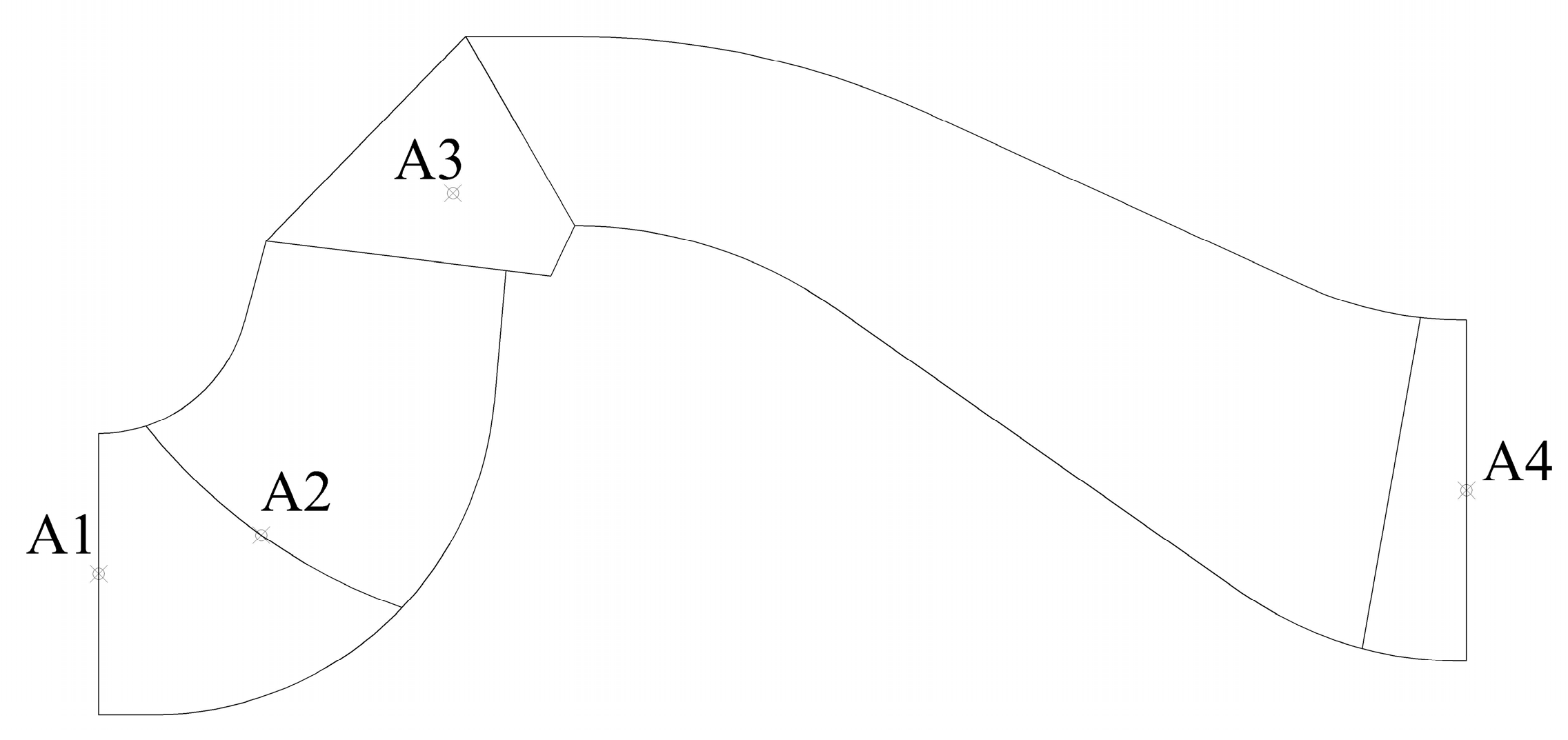
5.2.1. Pressure Pulsation Monitoring Point Configuration

Monitoring points A1–A4 were positioned on the mid-axis plane within the flow passage components. A1 is located at the impeller inlet, A2 is at the blade leading edge, A3 is in the middle of the cavity, and A4 is at the guide vane outlet. The arrangement of monitoring points is shown in Figure 12.

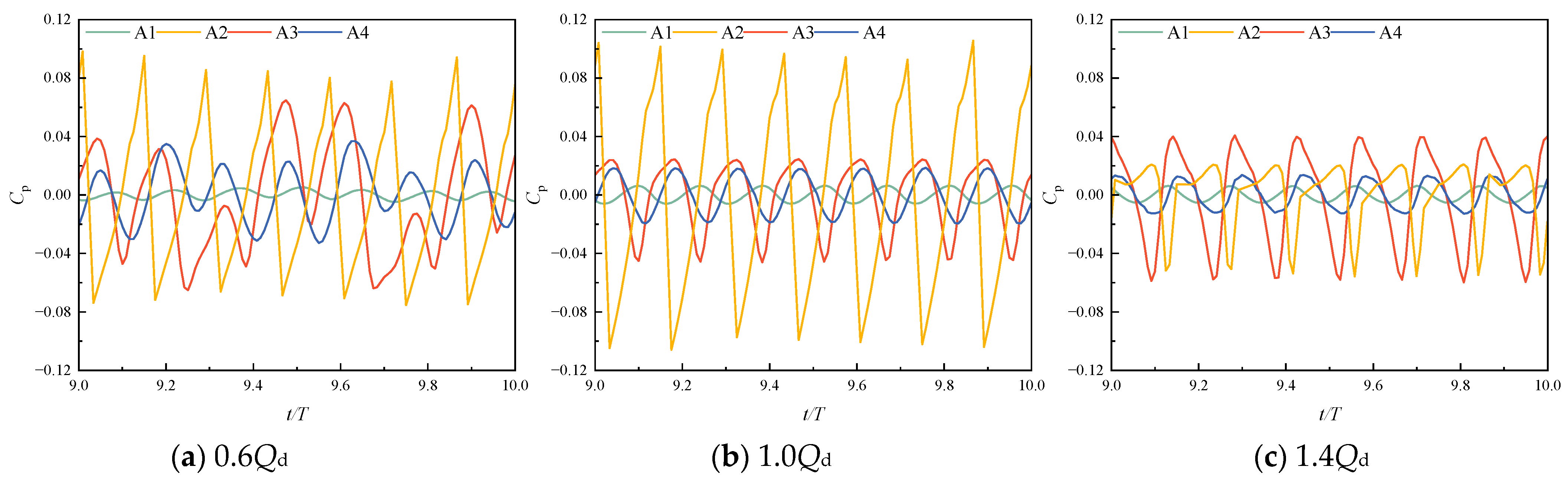
5.2.2. Time-Domain Analysis of Pressure Pulsation

Figure 13 depicts the time-domain plots of pressure pulsation at the monitoring points during the tenth rotation cycle, with the ordinate Cp. Figure 13a–c correspond to the pressure pulsation time-domain plots at flow rates of 0.6Qd, 1.0Qd, and 1.4Qd, respectively. Overall, Figure 13b indicates that at the 1.0Qd flow rate, the pressure pulsation at the monitoring points exhibits pronounced periodicity. In Figure 13a, it is observed that at the small flow rates, fluctuations in the amplitude of pulsations are observed at monitoring points A3 and A4. Figure 13c indicates that at large flow rates, the pressure pulsation at monitoring points A2 and A3 shows significant negative amplitudes.
The pressure pulsation at each monitoring point displays different variation patterns with the change in flow rate. This section individually analyzes the variation of pressure pulsation with flow rate at four monitoring points.
Monitoring Point A1: Figure 13 depicts that the fluctuation amplitude at monitoring point A1 is relatively small, presenting seven oscillation cycles which align with the number of impeller blades. Due to the simplification of the pump inlet pipe into a straight pipe, its impact on pulsation is minimal. Therefore, the main source of pressure pulsation at the impeller inlet is the interaction between the blades and the fluid. The amplitudes of pressure pulsation in Figure 13b,c are quite close. However, the pressure fluctuation amplitude in Figure 13a shows a trend of initially increasing and then decreasing. This observation suggests that at small flow rates, the fluid velocity decreases, leading to turbulence and backflow at the impeller inlet. The unstable flow of this portion of the fluid also becomes a source of pressure pulsation. With the increase in flow rate, the pulsation waveform tends to stabilize, and the peak appears later, indicating that large flow rates delay propagation of interaction between the blades and the fluid.
Monitoring point A2: Monitoring point A2 is located inside the impeller, where the amplitude of pressure fluctuations is high, showing strong periodicity, indicating that the primary cause of pulsation at A2 is the mutual interaction between the blades and the fluid. The pressure pulsation waveform at point A2 is highly similar at both small flow rates and rated flow rates. However, Figure 13c shows that there is a significant negative amplitude of pressure pulsation at large flow rates. In conjunction with the analysis in Section 5.1, it can be inferred that flow separation at the leading edge of the blades at large flow rates increases the negative amplitude of the pressure fluctuations.
Monitoring point A3: The monitoring point A3 is located in the middle of the cavity. Figure 13b shows that at rated flow rates, the pulsation waveform exhibits seven peaks and valleys. This observation signifies that the primary cause of pressure pulsation within the cavity is attributed to the rotor–stator interference between the impeller and guide vane, with the secondary cause possibly originating from the propagation of mutual interaction between the blades and the fluid. From Figure 13c, it is evident that the amplitude of pressure pulsation at monitoring point A3 increases, indicating a stronger rotor–stator interference at large flow rates. Figure 13a reveals that at small flow rates, the amplitude of pressure pulsation at monitoring point A3 exhibits irregular variations. Combining this observation with the streamline analysis of small flow rates in Section 5.1, it is indicated that the turbulent flow within the cavity also serves as one of the primary causes of internal pressure pulsation in the cavity.
Monitoring point A4: Monitoring point A4 is located at the exit of the guide vane; as stationary components, the guide vane itself has minimal influence on pulsations. Pulsations in the guide vane location are often propagated from the rotor components. Figure 13 illustrates a high degree of similarity in the pressure pulsation waveforms between A4 and A3, indicating that the primary cause of pressure pulsation at the guide vane exit is the rotor–stator interference. Figure 13c shows that at small flow rates, irregular fluctuations in amplitude occurred at point A4. This observation suggests that the unstable fluid flow also occurs at the guide vane outlet at small flow rates.

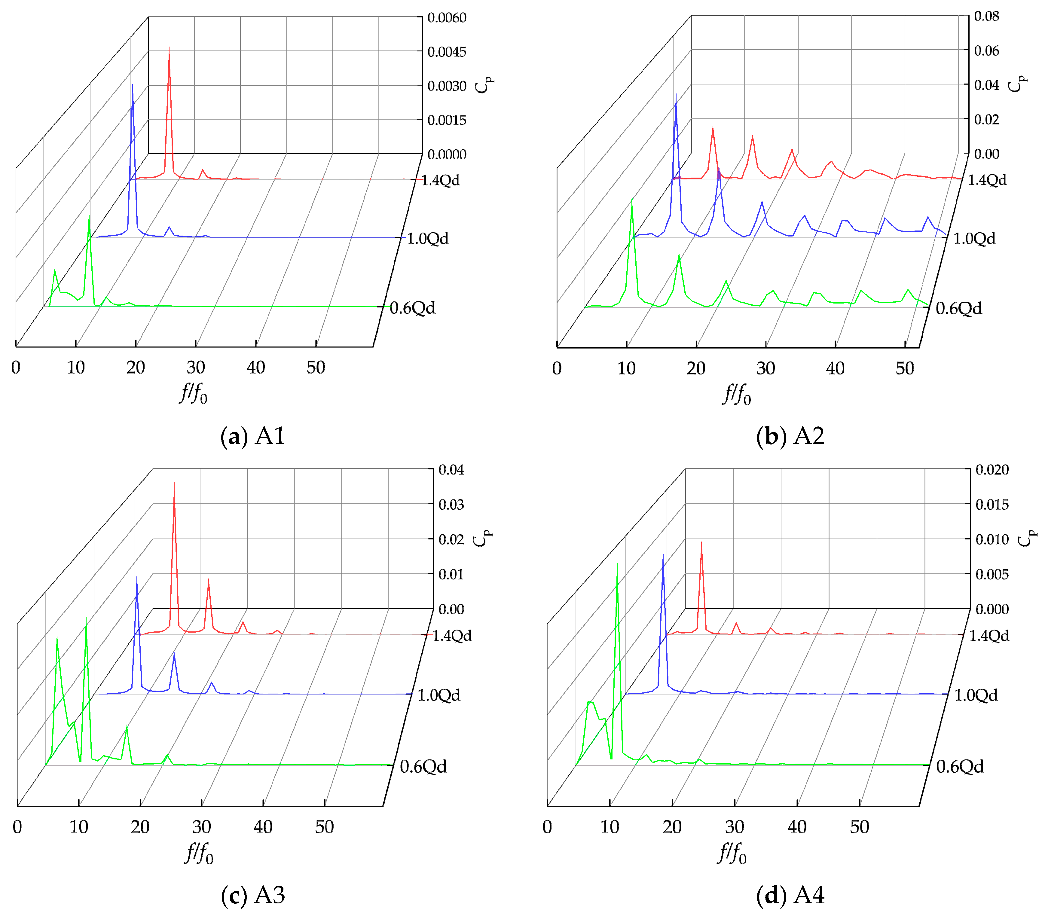
5.2.3. Pressure Pulsation Frequency Domain Analysis

Figure 14 displays the pressure pulsation frequency domain plots for monitoring points A1 to A4 during the tenth rotation cycle at flow rates of 0.6Qd, 1.0Qd, and 1.4Qd. The horizontal axis represents f/f0, while the vertical axis represents the amplitude of Cp. Figure 14a displays that the dominant frequency of pressure pulsation at monitoring point A1 appears at 6.94 f0 = 347 Hz for three flow rates, which is near the first blade frequency. In the flow rates of 1.0Qd and 1.4Qd, the subharmonics of the pulsation appear at 14.88f0 = 694 Hz, which corresponds to twice the blade frequency. At the small flow rates, the subharmonics of the pulsation occur at 0.994f0 = 50 Hz, corresponding to the shaft frequency. Simultaneously, a higher amplitude subharmonic is observed at 9.9 f0, indicating that the turbulence of the flow regime at the inlet at small flow rates increases the low-frequency component of pulsation. The pulsation at monitoring point A2 is mainly affected by the mutual interaction between the blades and the fluid. Consequently, in Figure 14b, the pulsation waveform exhibits a pronounced periodicity, and the amplitude of pulsation is also relatively high. The primary and subharmonic frequencies of pressure pulsation appear at the blade frequency, and the shaft rate magnetic field signal emerges in the high-frequency range. At large flow rates, flow separation occurs in the vicinity of A2, leading to a significant decrease in the amplitude of the blade frequency. Figure 14c shows that there is no shaft rate magnetic field signal in the high-frequency region, indicating that the pressure pulsation within the cavity is minimally influenced by the mutual interaction between the fluid and the impeller blades, with the main source being the rotor–stator interference. At small flow rates, the pressure pulsation in the low-frequency region at A3 exhibits irregular secondary frequency amplitudes similar to those at A1, indicating that turbulence inside the cavity has become one of the main causes of pulsation low-frequency signals. At the 1.4Qd flow rate, the increase in amplitude means that the rotor–stator interference becomes more pronounced at large flow rates. The primary cause of pressure pulsation at monitoring point A4 is the propagation of rotor–stator interference. Therefore, the waveform in Figure 14d is similar to that at monitoring point A3. But, at large flow rates, the amplitude of pulsation is smaller than that at the rated flow rates, signifying that an increase in flow rate weakens the propagation of pulsation caused by rotor–stator interference.

5.3. Entropy Generation Analysis

5.3.1. Entropy Generation Theory

According to the second law of thermodynamics, entropy generation is caused by irreversible processes such as heat transfer, friction, and flow viscous dissipation [25]. The fluid flow within a guide vane centrifugal pump is accompanied by various irreversible processes, leading to an increase in entropy generation. The fluid inside the pump is 25 °C water, which has a relatively high specific heat capacity. The flow within the pump can be simplified as isothermal motion, so the entropy generation in the flow process mainly originates from the combined effects of time-averaged velocity, fluctuating velocity, and wall effects [26].
The entropy generation rate due to time-averaged velocity, also known as the direct dissipation entropy generation rate, is calculated by the following formula:
S pro   , D ¯ = μ T 2 u ¯ x 2 + v ¯ y 2 + w ¯ z 2 +   v ¯ x + u ¯ y 2 + w ¯ x + u ¯ z 2 + v ¯ z + w ¯ y 2
In the equation, μ represents the dynamic viscosity of the fluid (kg·m−1·s−1); u, v, and w are the components of velocity in the Cartesian coordinate system’s x, y, and z directions, respectively, (m/s); T stands for temperature, K.
The entropy generation rate resulting from turbulent velocity fluctuations is also referred to as turbulent dissipation entropy generation rate, with the formula
S pro   , D = ρ ε T
In the equation, ε represents turbulent dissipation rate (m2/s3); ρ stands for fluid density (kg/m3). Based on the turbulent eddy frequency ω equation and turbulent kinetic energy k equation in the k-ω model, the formula for turbulent dissipation entropy generation rate evolves as S pro   , D = β ρ ω k T ,where β = 0.09; ω represents the turbulent eddy frequency (s−1); k represents turbulent kinetic energy (m2/s2). Hence, the local total entropy generation rate can be expressed as
S pro   , D = S pro   , D + S pro   , D ¯
The entropy generation rate is influenced by wall effects, and the formula for calculating the wall dissipation entropy generation rate is
S pro ,   W = τ v T
In the equation, τ represents the wall shear stress (Pa) and v represents the velocity near the wall (m/s). The total entropy production can be obtained by summing up the above three entropy production rates integrated over the simulation domain:
Δ S pro = V S pro   , D ¯ dV + V S pro   , D dV + A S pro ,   W dA
As analyzed above, from the analysis above, it can be concluded that at nonrated flow rates, the pump experiences unstable flow inside, leading to energy losses. To further investigate the characteristics of energy losses within the pump, an analysis was conducted on the local total entropy generation rate and streamline of the impeller, cavity, and guide vanes, respectively.

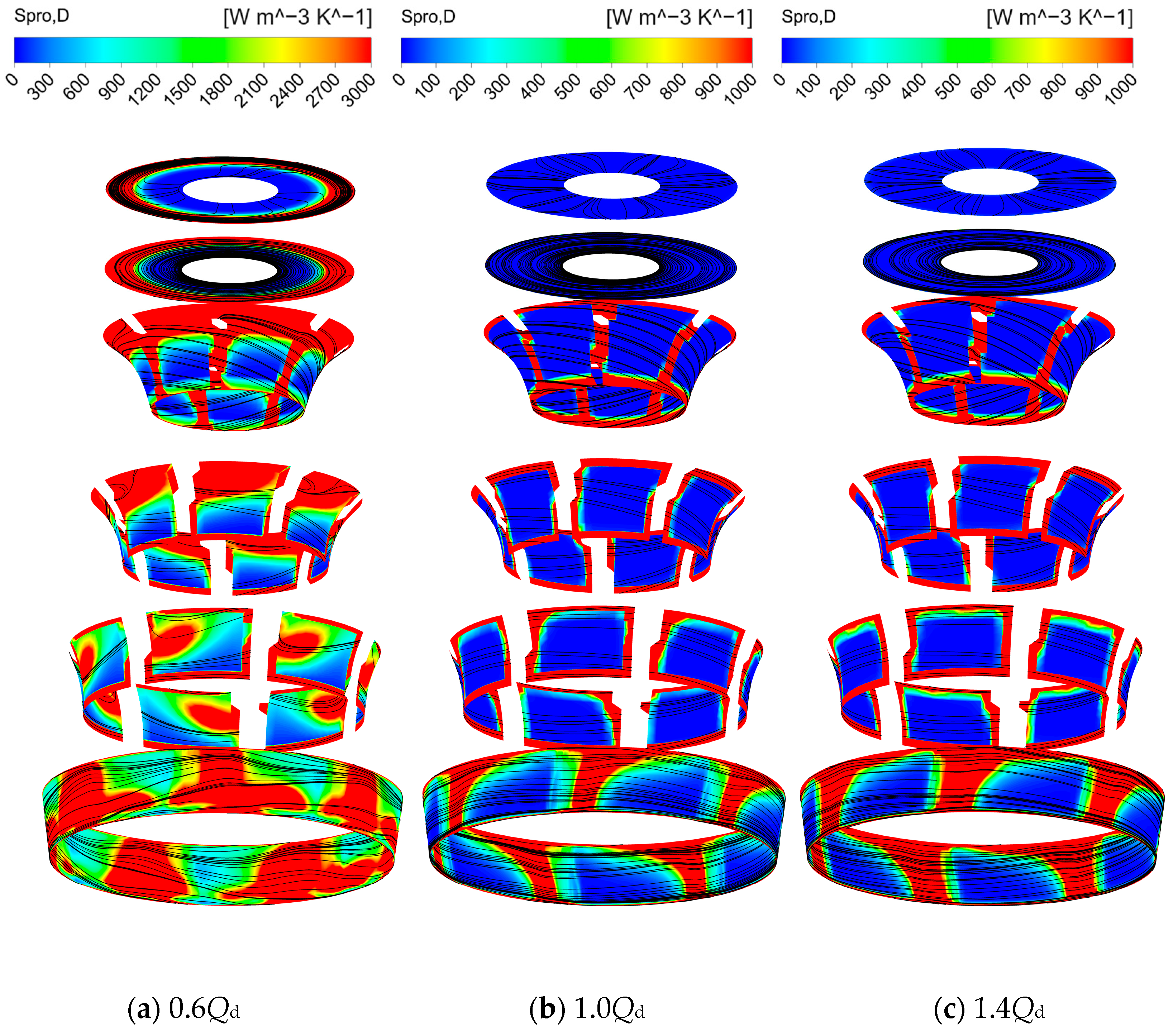
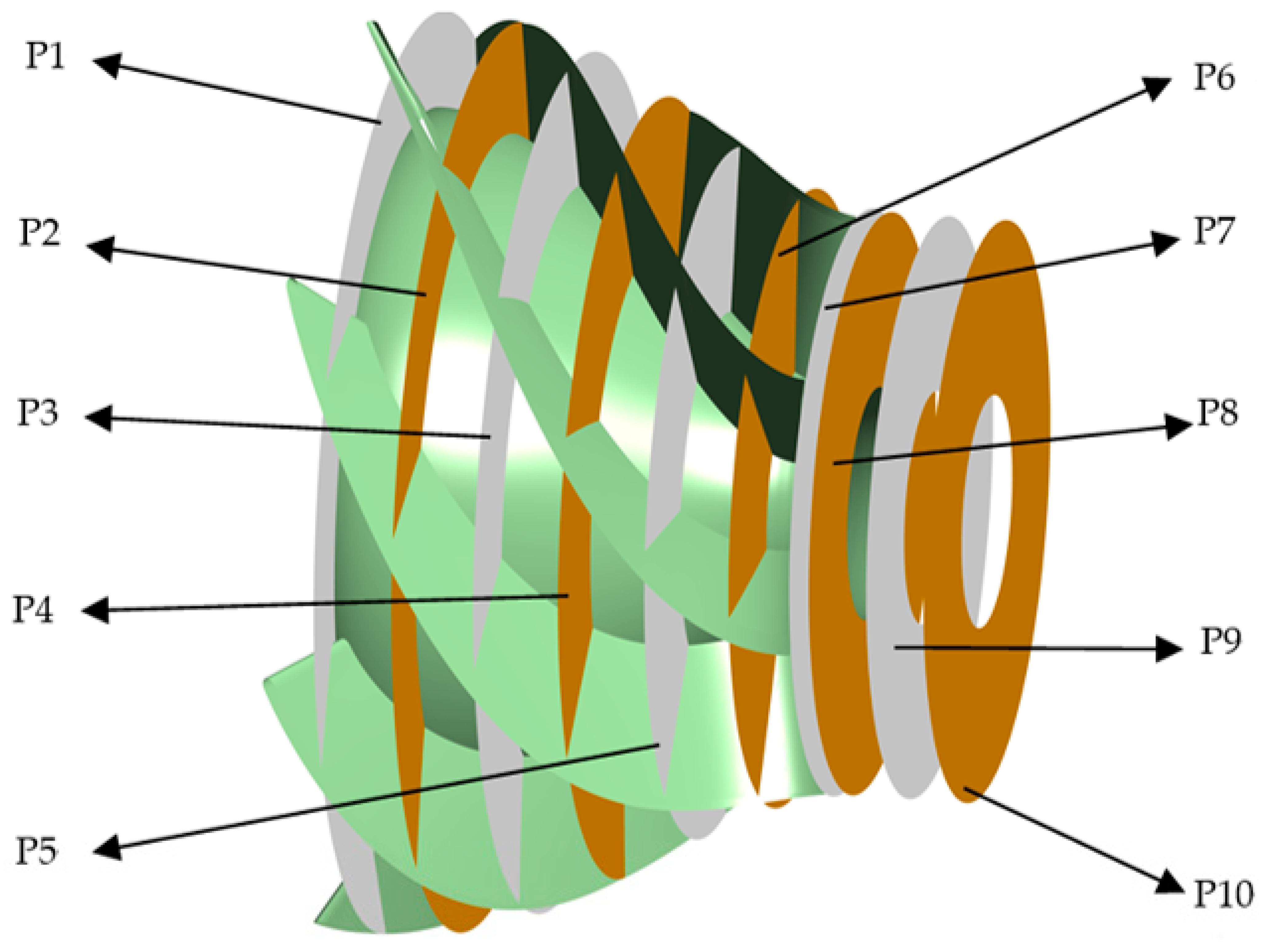
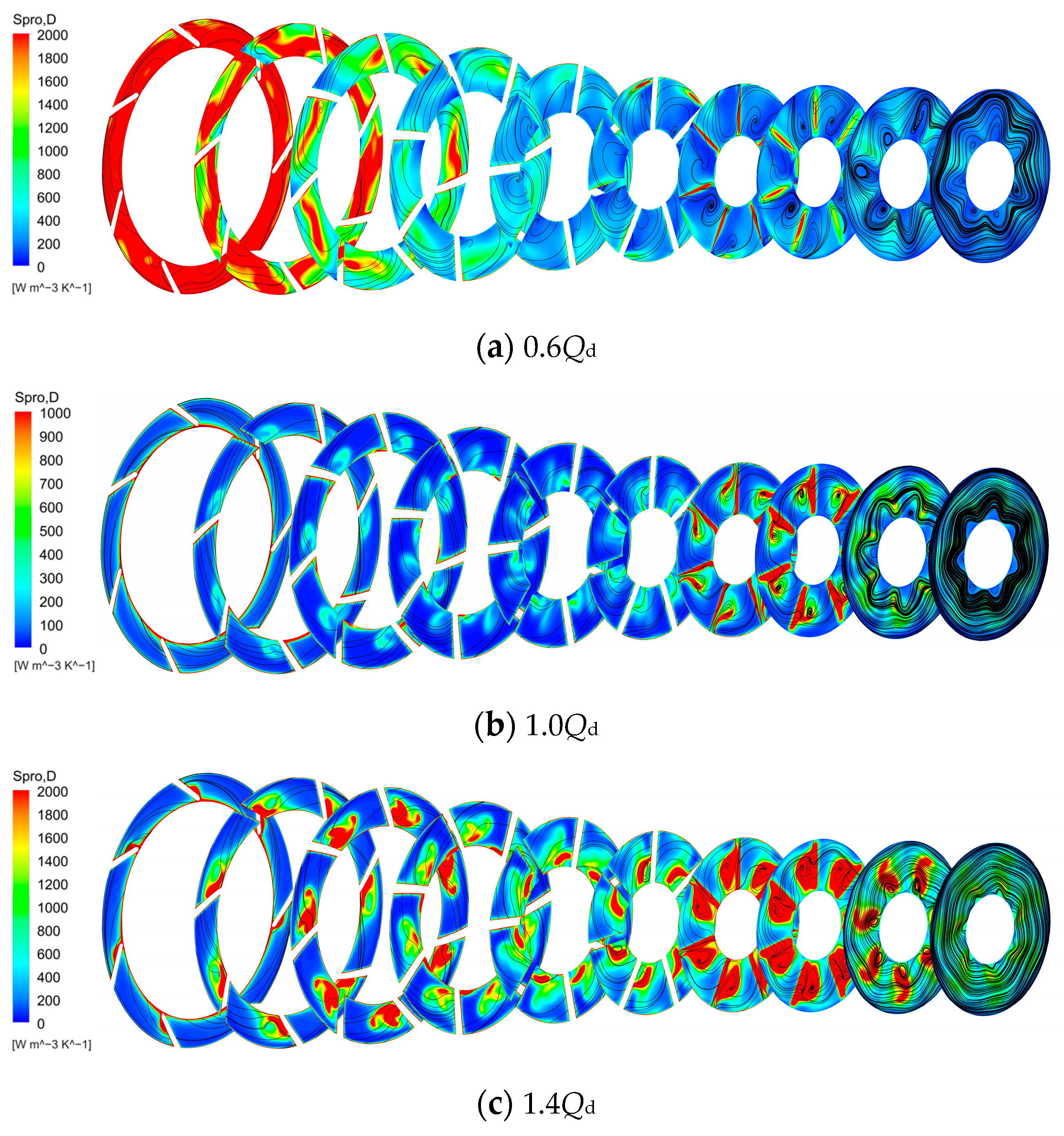
5.3.2. Analysis of Flow and Entropy Generation within the Impeller

To thoroughly analyze the internal flow characteristics within the impeller, cross sections I–VI are established, as shown in Figure 15. Cross section I is the inlet pipe cross section 10 mm away from the impeller inlet; cross section II corresponds to the impeller inlet surface; cross section III is located at the leading edge of the impeller blade; cross sections III to V are all impeller flow passages, they are generated by the rotation of curves in the impeller axial projection drawing, as shown in Figure 15c; cross section VI is the impeller outlet surface.
Figure 16 displays the local total entropy generation rate and streamline at cross sections I to VI at various flow rates. In order to comprehensively observe the cross section data, a translation operation was applied to these cross sections. Figure 16b,c demonstrate that at large flow and rated flow rates, energy losses of impeller are primarily concentrated near the blade, hub, and shroud. Additionally, at large flow rates, the high-entropy region at the cross section VI expands further. This indicates that with an increase in flow rate, the flow separation phenomenon intensifies near the trailing edge of the blades, leading to an increase in energy loss. In terms of streamlines, the fluid within the impeller flows uniformly in the direction of the blade rotation. The streamline on section I points from the inner wall to the outer wall and is divided into seven parts. It means that at flow rates of 1.0Qd and 1.4Qd, the fluid at the tail end of the inlet pipe is affected by the mutual interaction between the impeller blades and the fluid. Figure 16a depicts that at small flow rates, the entropy production rate of the fluid within the impeller increases, particularly at cross sections III and IV near the shroud, where the high-entropy region expands further. This indicates that the flow area at cross sections III and IV is relatively large and the fluid cannot fill this space at small flow rates, further intensifying fluid instability. The streamline in Figure 16a shows the occurrence of vortices at cross section IV, which perfectly overlaps with the high-entropy region. This suggests that the energy loss at cross section IV is caused by these vortices. At cross section V, the high-entropy region shifts towards the vicinity of the backside of the blades. This conveys that as the fluid velocity decreases, instability phenomenon occurs in the low-speed region of the fluid at the backside of the blades. This is consistent with the streamline analysis at small flow rates in Section 5.1. This unstable fluid is the primary cause of energy loss at cross section V. From Figure 16a, it can also be observed that high-entropy regions appear on the outer sides of cross sections I and II. Additionally, the streamlines on Section I show that fluid at this location begins to exhibit circumferential motion. This indicates that at small flow rates, the fluid at the tail end of the inlet pipe is more susceptible to the mutual interaction between the blades and the fluid.

5.3.3. Internal Flow and Entropy Generation Analysis within the Cavity

The cavity is a narrow region between the impeller and the guide vane, where the flow state undergoes significant changes. In order to investigate the flow patterns and entropy generation characteristics within the cavity, cross sections were established along the circumferential direction at intervals of 15 degrees, as shown in Figure 17. A total of 24 cross sections were configured. In Figure 17b, the section boundaries are indicated, where “inlet” represents the interface between the impeller and the cavity, and “outlet” refers to the interface between the spatial guide vane and the cavity. “Wall” represents the pump casing adjacent to the cavity. The fluid flows from the “inlet” of the cavity to the “outlet” of the cavity.
Figure 18 depicts the local entropy generation rate distribution and streamlines for the cavity cross sections at different flow rates. In order to investigate the evolution of the flow field within the cavity over one rotation cycle, the tenth rotation cycle T10 of the impeller is divided into four quarters. Figure 18b illustrates that, at the rated flow rates, the high-entropy region within the cavity is primarily located near the cavity walls. This indicates that the energy loss within the cavity is mainly attributed to the variations in fluid velocity and direction. The streamline diagram reveals that small vortices form near some of the wall surfaces, and the positions of these vortices remain consistent throughout the entire cycle. Additionally, small high-entropy regions also appear at the inlet of some cross sections. Incorporating the evolution of fluid flow from 1/4 T10 to 1 T10, it is observed that these high-entropy regions are consistently present at the sections near the trailing edge of the impeller blades. This signals the occurrence of flow separation near the trailing edge of the blades at the rated flow rates. Compared to Figure 18b, in Figure 18c, the streamlines remain unchanged, and the high-entropy regions expand further. On the one hand, the expansion of the high-entropy regions at the inlet of the cross sections is due to the intensified flow separation caused by the increase in flow rate. On the other hand, the fluid inside the cavity is primarily influenced by the rotor–stator interference. The expansion of the high-entropy regions at large flow rates indicates that the rotor–stator interference becomes more intense. This is consistent with the analysis of pressure pulsation at monitoring point A3 in Section 5.2.2. The streamlines in Figure 18a reveal that at small flow rates, the flow within the cavity becomes more turbulent. Additionally, the high-entropy zones exhibit an irregular distribution. Combining the analysis of pressure pulsation at point A3, it is found that at small flow rates, the energy loss within the cavity is primarily attributed to turbulence and rotor–stator interference. The distribution of streamlines at the cross sections throughout the entire cycle illustrates the evolution process of vortices within the cavity. At 1/4 T10 and 3/4 T10 instants, there are only a few vortices inside the cavity. However, at 1/2 T10 and 1 T10 instants, the number of vortices increases, and their level of turbulence intensifies. At small flow rates, this vortex motion not only generates significant energy loss in the cavity section but also propagates the turbulence downstream to the guide vane.

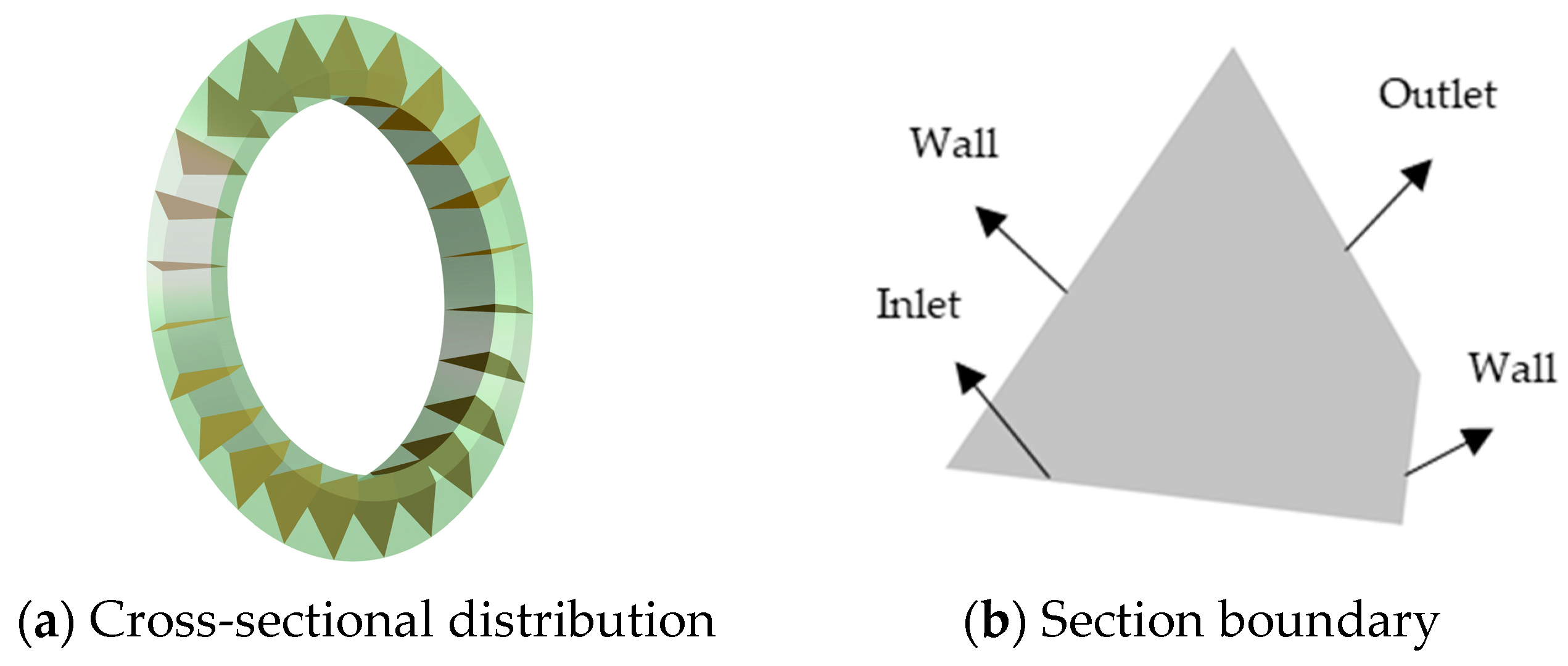
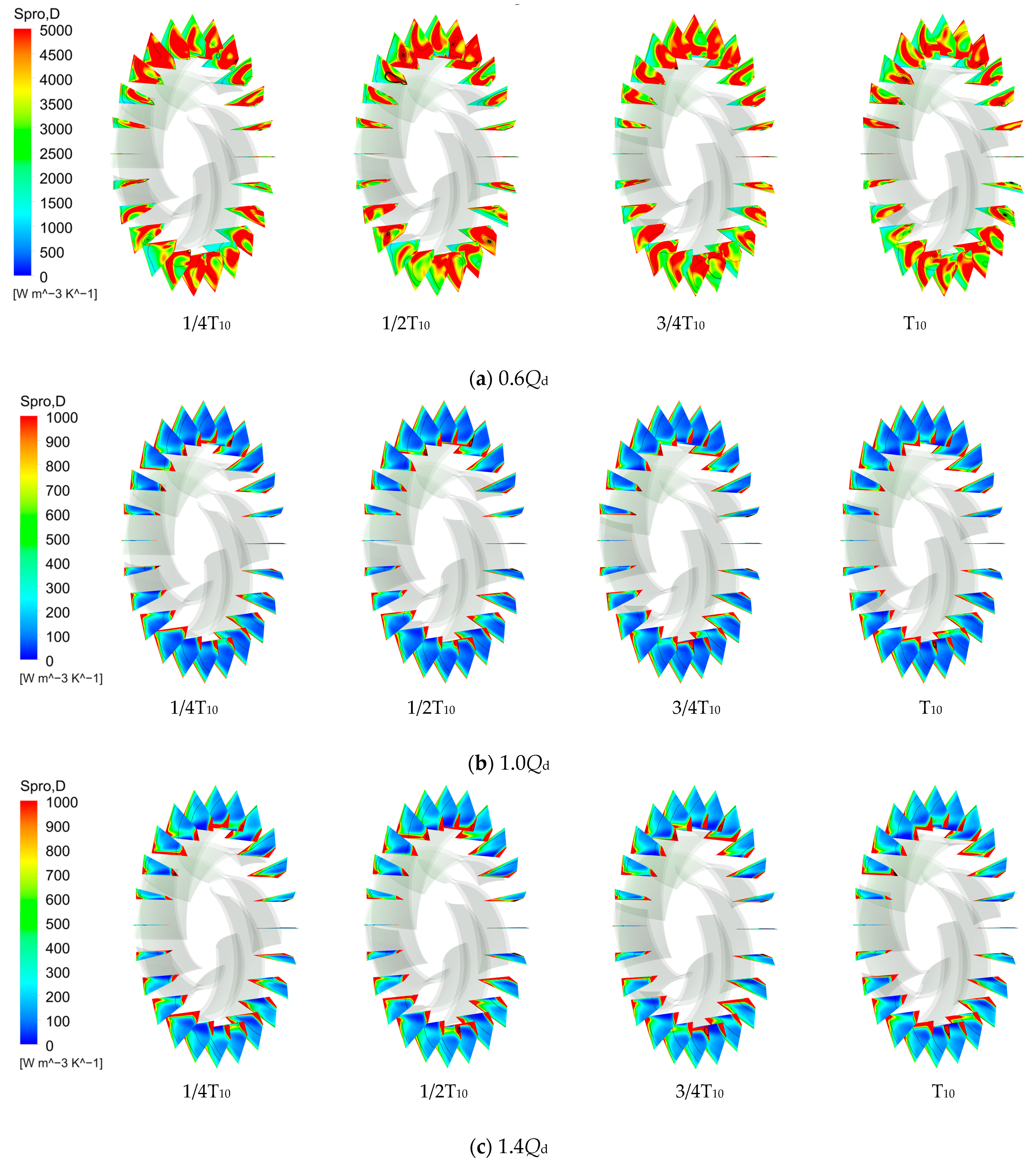
5.3.4. Analysis of Internal Flow and Entropy Generation in Guide Vane

For a detailed analysis of the flow within the guide vane, cross sections P1–P10 are established along the main axis direction. P1 represents the leading edge of the blades, P7 corresponds to the trailing edge of the blades, and there is a 20 mm spacing between the cross sections P1–P7. P8 corresponds to the outlet of the guide vane, while P9 and P10 represent sections within the outlet pipe, situated at distances of 15 mm and 30 mm from the outlet of the guide vane. The arrangement of these cross sections is illustrated in Figure 19.
Figure 20 displays the local total entropy generation distribution and streamlines at cross sections P1–P10 at various flow rates. In order to comprehensively observe the sectional data, each cross section was subjected to translational motion. From Figure 20b, it can be observed that the local entropy generation at each cross section is at a relatively low level, indicating low energy loss within the guide vane at rated flow rates. The streamline distribution on cross sections P1 to P6 is uniform and does not form vortices. Cross sections P7 and P8 are located, respectively, at the trailing edge of the blades and the outlet of the guide vane. The fluid at this location is influenced by the blade structure, leading to flow separation at the blade trailing edge and the formation of seven vortices, and resulting in energy loss. At cross sections P9 and P10, the vortices gradually dissipate, and the flow returns to a stable state. In summary, at rated flow rates, the flow of fluid within the guide vane tends to stabilize and the energy loss is relatively low, with only unstable flow occurring at the trailing edge of the blades. As indicated by Figure 20a, at small flow rates, the local total entropy generation rate at P1–2 is significantly high. In conjunction with the analysis in Section 5.3.3, it can be found that the fluid flow inside the cavity is extremely turbulent at small flow rates, generating irregular vortices. This turbulence further affects the fluid flow within the guide vane, resulting in energy loss of fluid within the guide vane. In Figure 20a, only a small portion of high-entropy regions appears at the trailing edge of the blades; this indicates that as the flow rate decreases, the flow separation at the trailing edge is alleviated. In cross sections P9 and P10, vortices still exist, indicating that at small flow rates, the unstable flow is more prone to propagation. At large flow rates, Figure 20c shows a further increase in entropy generation rate within the guide vane, and the distribution of high-entropy regions and streamlines is similar to that at rated flow rates. The distribution of entropy generation rates and the flow pattern are both similar to those observed at rated flow conditions. The only difference is mainly caused by the leading and trailing edges of the blades. From section P7, it can be observed that as the flow rate increases, flow separation at the rear edge of the blade intensifies, causing propagation of high-entropy production areas to nearby areas. Unlike the rated flow rates, this turbulence even affects the vicinity of cross section P6 at large flow rates. From cross section P1, it can be observed that the high-entropy regions at the leading edge of the blade expand compared to the rated flow rates. Simultaneously, small vortices appear within the high-entropy regions and further develop at sections P2–3. This indicates that with an increase in flow rate, there are localized low-pressure regions on the leading edge of the blades. This further illustrates the presence of flow separation at this location, which further develops along the flow direction and affects the subsequent flow until the middle section P5 of the guide vane.

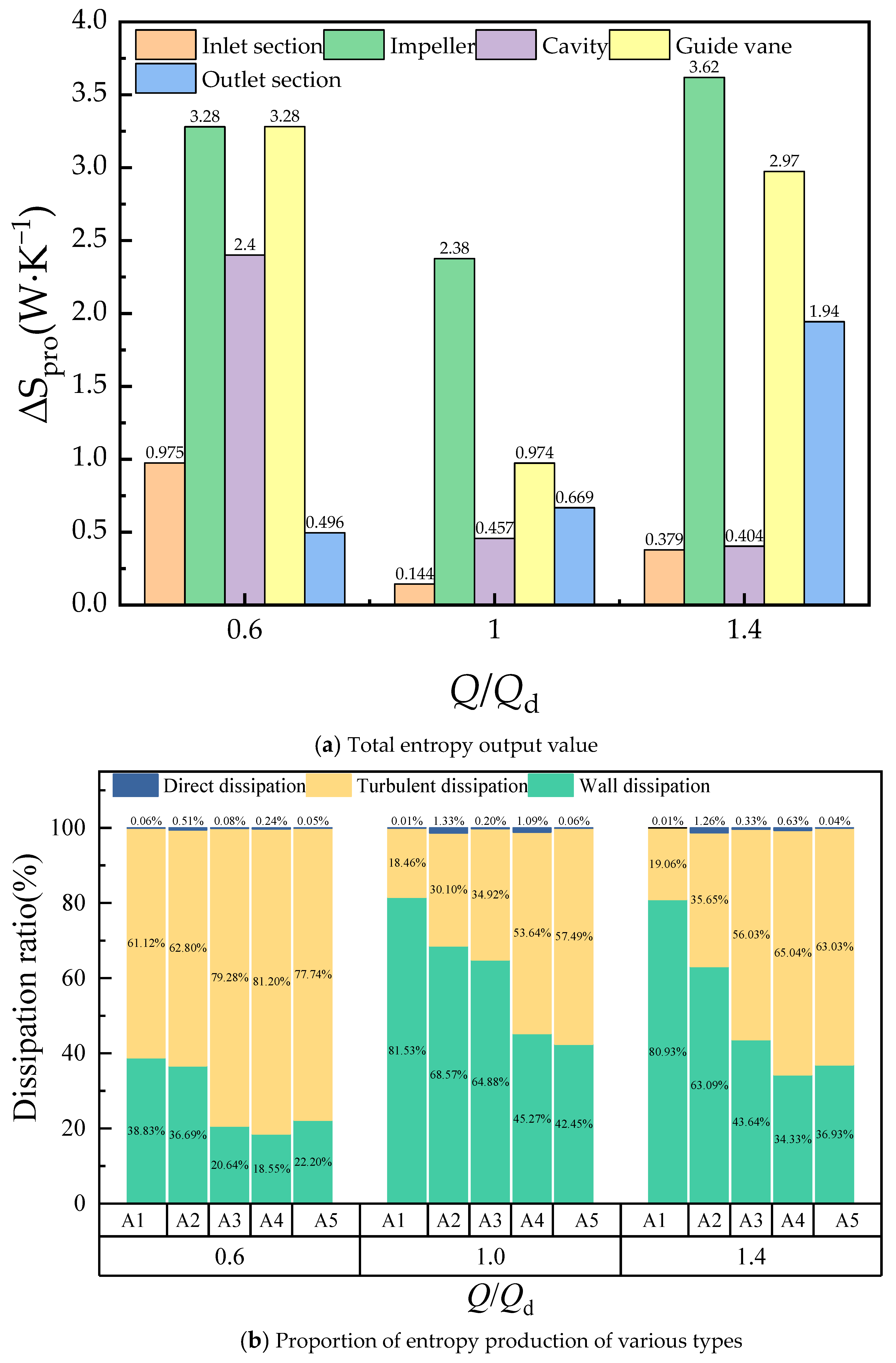
5.3.5. Analysis of Entropy Generation in Flow Components

Qualitative analysis was conducted on the entropy generation characteristics of the fluid within the flow passage components in the previous section. To quantitatively analyze the energy loss of the pump, the total entropy generation for each component was calculated. Figure 21a presents the total entropy generation for various components at the flow rates of 0.6Qd, 1.0Qd, and 1.4Qd. Figure 21b represents the proportion of total entropy generation contributed by various categories of entropy generation within each flow passage component. The components are represented as A1–A5 for the inlet pipe, impeller, cavity, guide vanes, and outlet pipe, respectively. Figure 21b illustrates that the proportion of direct dissipation to the total entropy generation is extremely small. The primary causes of entropy generation within the pump are turbulent dissipation and wall dissipation. Therefore, the local entropy generation rate in Section 5.3.1 can be approximately regarded as the turbulent dissipation entropy generation rate. At the rated flow rates, Figure 21 shows that the main cause of entropy generation is the impeller, with wall dissipation being the primary type of entropy generation within the impeller. The main reasons are as follows: (1) As a rotating component, the fluid velocity inside the impeller is very high, which increases the friction between the fluid and the blade surface, resulting in more wall dissipation. (2) Compared to other flow passage components, the impeller has a more complex structure. Thus, the impeller has a larger contact area with the fluid. This leads to stronger friction effects, consequently increasing the proportion of wall dissipation. At the large flow rates, Figure 21a shows that the impeller, guide vane, and outlet pipe have become the main sources of entropy generation. Meanwhile, it illustrates that the proportion of three types of entropy production within the impeller has not changed in Figure 21b. According to the analysis in Section 5.3.2 above, at large flow rates, the local total entropy generation rate within the impeller increases, indicating an elevation in turbulent dissipation. Hence, the total entropy generation at the impeller increases from 2.38 W·K−1 to 3.62 W·K−1. Turbulent dissipation accounts for about 65% of the total entropy production of the guide vanes and outlet pipes, and it indicates that the turbulence generated by the impeller rotation undergoes significant development as it passes through the cavity, guide vanes, and outlet pipe. This leads to a more chaotic fluid flow within the downstream components. According to the analysis in Section 5.3.4 above, the local total entropy generation rate of the guide vane and outlet pipe significantly improved compared to the rated flow rates, resulting in a 210% increase in the total entropy production of the guide vane and outlet pipe at large flow rates. Figure 21 reveals that the main components contributing to entropy generation within the pump are the impeller, cavity, and guide vanes. Among them, turbulent dissipation is the main contributor to entropy generation at small flow rates, while wall dissipation decreases further due to the reduction in flow velocity. According to the previous analysis, it can be concluded that the unstable fluid flow at low flow rates is the primary reason for the increase in turbulent dissipation. Compared to the rated flow rates, the total entropy production in the cavity increases by approximately 421%, which is the largest increase among all components. This indicates that the cavity is the region where turbulent phenomena are most pronounced within the pump. Overall, in terms of the entire pump, throughout the process from the inlet to the outlet, turbulence continues to develop. Consequently, the proportion of turbulent dissipation in the entropy production of downstream components gradually increases. In terms of flow variation, as the flow rate increases, it leads to a gradual increase in wall dissipation. Regarding turbulent dissipation, with the increase in flow rate, turbulent dissipation initially decreases and then increases. Turbulent dissipation at small flow rates is primarily caused by the fluid’s unstable flow, while at large flow rates, the primary source of turbulent dissipation is the flow separation occurring at the leading and trailing edges of the blades. The total entropy production is the lowest at rated flow rates and the highest at small flow rates. Therefore, it is advisable to avoid operating the guide vane centrifugal pump at small flow rates whenever possible.

6. Conclusions

(1)
The guide vane centrifugal pump was selected as the research subject, and the number of blades, blade wrap angle, blade outlet angle, and axial and radial distances between the guide vane and impeller were considered as design variables. The pump head and efficiency were treated as response variables. Based on the Box–Behnken design method and CFX numerical simulation results, the function equation between design variables and response variables was obtained. Additionally, the influence of each factor on the response variables was analyzed. It was observed that all five single-factor variables had a significant impact on the head and efficiency. There are interactions among the factors, however; compared to single factor and single-factor quadratic, two-factor interaction terms are less significant.
(2)
Based on the RSM, a quadratic polynomial equation was established, and it was found that the optimal combination of guide vane centrifugal structural parameters is Z = 7, β2 = 23.8°, φ1 = 100.7°, ∆r = 22.814 mm, and ∆z = 13.838 mm. The simulated values of the original model and the optimized model are in close agreement with the predicted values from the RSM. Additionally, the optimized model exhibits an increase of 2.5845 m in head and a 2.88% improvement in efficiency compared to the original model. This indicates that the RSM is capable of accurately reflecting the complex nonlinear relationships between the structural parameters of the guide vane centrifugal pump and the optimization objectives. It provides an intuitive and effective optimization approach for the design of guide vane centrifugal pumps.
(3)
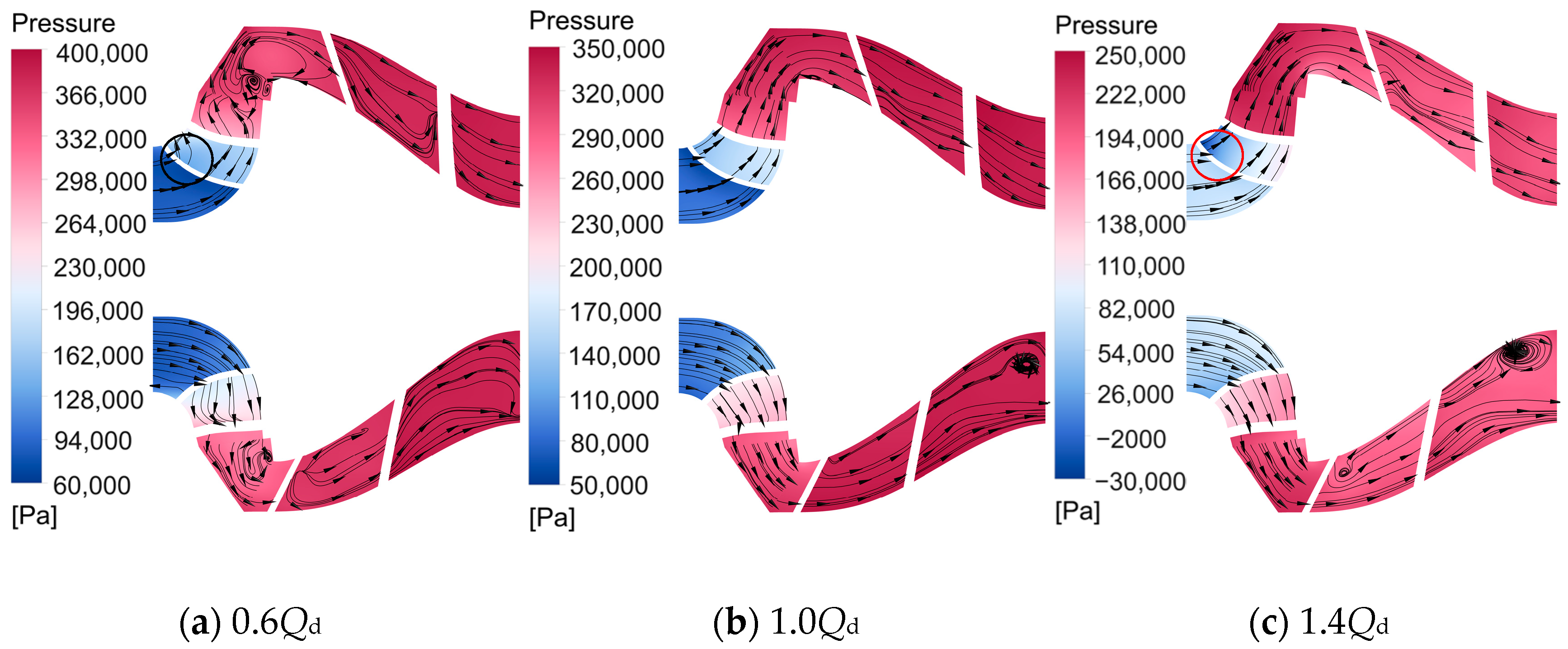
Analyzing the transient flow characteristics of the optimized model: At rated flow rates, the fluid flow within the pump remains stable. At large flow rates, flow separation is prone to occur at the leading and trailing edges of the blades. At small flow rates, the fluid flow within the pump becomes more turbulent. The pressure fluctuations within the impeller are primarily caused by the interaction between the blades and the fluid. For the cavity and guide vane, pressure fluctuations predominantly result from the rotor–stator interference. These pressure fluctuations exhibit strong periodicity, with their dominant frequencies situated around the blade frequency. At small flow rates, the turbulence generated by the unstable flow inside the pump also becomes one of the main causes of pressure fluctuations. At large flow rates, fluid separation occurs at the leading and trailing edges of the blades, resulting in variations in pressure pulsation amplitude. In the centrifugal pump with guide vanes, the turbulent and wall dissipations contribute higher values compared with the direct dissipation. At the rated flow rates, the entropy generation is concentrated in the impeller. At large flow rates, the increase in fluid velocity leads to an augmentation in wall friction dissipation and intensifies the flow separation, resulting in an escalation of turbulent dissipation at the leading and trailing edges of the blades. At small flow rates, the turbulence generated by the unstable fluid flow becomes the primary source of turbulent dissipation. At this point, the entropy production value of the guide vane centrifugal pump is the highest.

Author Contributions

Conceptualization, W.C.; methodology, W.C. and H.W.; software, H.W. and X.Y.; formal analysis, H.W.; writing—original draft preparation, H.W.; writing—review and editing, W.C. and X.L.; supervision, W.C.; investigation (performing the experiments), W.C., and H.W. All authors have read and agreed to the published version of the manuscript.

Funding

This work was supported by National Key Research and Development Program (Grant No. 2020YFC1512405) and Jiangsu Provincial Key Research and Development Program (Grant No. BE2020330).

Institutional Review Board Statement

Not applicable.

Informed Consent Statement

Not applicable.

Data Availability Statement

Not applicable.

Conflicts of Interest

The authors declare no conflict of interest.

Abbreviations

QdDesign flow rate, m3/h
HdDesign head, m
nDesign speed, r/min
nsSpecific speed
HHead, m
ηEfficiency, %
DjImpeller inlet diameter, mm
D2Impeller outlet diameter, mm
b2Impeller outlet width, mm
DhImpeller hub diameter, mm
β1Impeller blade inlet angle, °
β2Impeller blade outlet angle, °
φ1Impeller blade wrap angle, °
b3Guide vane inlet width, mm
φ2Guide vane wrap angle, °
α3Guide vane inlet setting angle, °
α4Guide vane outlet setting angle, °
LGuide vane axial length, mm
zAxial distance between impeller and guide vane, mm
rRadial distance between impeller and guide vane, mm
ZNumber of impeller blades
S2Variance
R²Coefficient of determination
R a d j 2 Adjusted coefficient of determination
R p r e 2 Predictive coefficient of determination
HaHead coefficient, m
PinletAverage pressure at the inlet surface, Pa
PaveAverage pressure at any cross section of the guide vane centrifugal pump, Pa.
CpNondimensional pressure fluctuation coefficient
pStatic pressure at the monitoring point, Pa.
p ¯ Time-averaged pressure at the monitoring point during the computation period, Pa.
ρFluid density, kg/m³
u2Circumferential velocity at the impeller outlet, m/s
f0Impeller rotational frequency
S pro   , D ¯ Direct dissipation entropy generation rate, kg·m−1·s−3·K−1
S pro   , D Turbulent dissipation entropy production rate, kg· m−1·s−3·K−1
S pro ,   W Wall dissipation entropy generation rate, kg·s−3·K−1
S pro   , D Local total entropy generation rate, kg·m−1·s−3·K−1
Δ S pro Total entropy production, W·K−1
μDynamic viscosity of the fluid, kg·m−1·s−1
u, v, wComponents of velocity in the Cartesian coordinate system’s x, y, and z directions, respectively, m/s
TTemperature, K
ωTurbulent eddy frequency, s−1
kTurbulent kinetic energy, m2/s2
τ Wall shear stress, Pa
v Velocity near the wall, m/s
Acronyms
CFDComputational fluid dynamics
DOEDesign of experiment
RSMResponse surface method
SSMSurrogate model method

References

  1. Shi, W.; Zhou, L.; Lu, W.; Xu, L.; Li, W. Numerical Simulation and Experimental Study of Different Stages Deep-Well Centrifugal Pump. J. Comput. Theor. Nanosci. 2013, 10, 2897–2901. [Google Scholar] [CrossRef]
  2. Zhou, L.; Shi, W.; Lu, W.; Hu, B.; Wu, S. Numerical Investigations and Performance Experiments of a Deep-Well Centrifugal Pump With Different Diffusers. J. Fluids Eng. 2012, 134, 071102. [Google Scholar] [CrossRef]
  3. Xuran, G.; Puyu, C.; Yang, W.; Rui, Z.; Yefu, W. Linear control design and internal flow analysis of diffuser trailing edge based on CFD. J. Drain. Irrig. Mach. Eng. 2021, 39, 1210–1217. [Google Scholar]
  4. Zailun, L.; Sanzhen, W.; Jingmin, Z.; Jinxuan, W. Optimal design of geometric parameters of diffuser inlet under optimal working conditions. J. Drain. Irrig. Mach. Eng. 2021, 39, 973–980. [Google Scholar]
  5. Kim, S.; Kim, Y.-I.; Kim, J.-H.; Choi, Y.-S. Design optimization for mixed-flow pump impeller by improved suction performance and efficiency with variables of specific speeds. J. Mech. Sci. Technol. 2020, 34, 2377–2389. [Google Scholar] [CrossRef]
  6. Heo, M.-W.; Kim, K.-Y.; Kim, J.-H.; Choi, Y.S. High-efficiency design of a mixed-flow pump using a surrogate model. J. Mech. Sci. Technol. 2016, 30, 541–547. [Google Scholar] [CrossRef]
  7. Safikhani, H.; Khalkhali, A.; Farajpoor, M. Pareto based multi-objective optimization of centrifugal pumps using CFD, neural networks and genetic algorithms. Eng. Appl. Comput. Fluid Mech. 2011, 5, 37–48. [Google Scholar] [CrossRef]
  8. Alawadhi, K.; Alzuwayer, B.; Mohammad, T.A.; Buhemdi, M.H. Design and Optimization of a Centrifugal Pump for Slurry Transport Using the Response Surface Method. Machines 2021, 9, 60. [Google Scholar] [CrossRef]
  9. Wang, W.J.; Yuan, S.Q.; Pei, J.; Zhang, J.F. Optimization of the diffuser in a centrifugal pump by combining response surface method with multi-island genetic algorithm. Proc. Inst. Mech. Eng. Part E J. Process Mech. Eng. 2016, 231, 191–201. [Google Scholar] [CrossRef]
  10. Kim, J.-H.; Lee, H.-C.; Kim, J.-H.; Yoon, J.-Y.; Choi, Y.-S. Design techniques to improve the performance of a centrifugal pump using CFD. J. Mech. Sci. Technol. 2015, 29, 215–225. [Google Scholar] [CrossRef]
  11. Nataraj, M.; Singh, R.R. Analyzing pump impeller for performance evaluation using RSM and CFD. Desalination Water Treat. 2014, 52, 6822–6831. [Google Scholar] [CrossRef]
  12. Thakkar, S.; Vala, H.; Patel, V.K.; Patel, R. Performance improvement of the sanitary centrifugal pump through an integrated approach based on response surface methodology, multi-objective optimization and CFD. J. Braz. Soc. Mech. Sci. Eng. 2021, 43, 24. [Google Scholar] [CrossRef]
  13. Wu, C.; Yang, J.; Yang, S.; Wu, P.; Huang, B.; Wu, D. A Review of Fluid-Induced Excitations in Centrifugal Pumps. Mathematics 2023, 11, 1026. [Google Scholar] [CrossRef]
  14. Posa, A.; Lippolis, A. Effect of working conditions and diffuser setting angle on pressure fluctuations within a centrifugal pump. Int. J. Heat Fluid Flow 2019, 75, 44–60. [Google Scholar] [CrossRef]
  15. Shibata, A.; Hiramatsu, H.; Komaki, S.; Miyagawa, K.; Maeda, M.; Kamei, S.; Hazama, R.; Sano, T.; Iino, M. Study of flow instability in off design operation of a multistage centrifugal pump. J. Mech. Sci. Technol. 2016, 30, 493–498. [Google Scholar] [CrossRef]
  16. Qi, H.; Li, W.; Ji, L.; Liu, M.; Song, R.; Pan, Y.; Yang, Y. Performance optimization of centrifugal pump based on particle swarm optimization and entropy generation theory. Front. Energy Res. 2023, 10, 1094717. [Google Scholar] [CrossRef]
  17. Osman, M.K.; Wang, W.; Yuan, J.; Zhao, J.; Wang, Y.; Liu, J. Flow loss analysis of a two-stage axially split centrifugal pump with double inlet under different channel designs. Proc. Inst. Mech. Eng. Part C J. Mech. Eng. Sci. 2019, 233, 5316–5328. [Google Scholar] [CrossRef]
  18. Huang, P.; Appiah, D.; Chen, K.; Zhang, F.; Cao, P.; Hong, Q. Energy dissipation mechanism of a centrifugal pump with entropy generation theory. Aip Adv. 2021, 11, 045208. [Google Scholar] [CrossRef]
  19. Böhle, M.; Fleder, A.; Mohr, M. Study of the losses in fluid machinery with the help of entropy. In Proceedings of the 16th International Symposium on Transport Phenomena and Dynamics of Rotating Machinery, Honolulu, HI, USA, 10–15 April 2016. [Google Scholar]
  20. Melzer, S.; Pesch, A.; Schepeler, S.; Kalkkuhl, T.; Skoda, R. Three-Dimensional Simulation of Highly Unsteady and Isothermal Flow in Centrifugal Pumps for the Local Loss Analysis Including a Wall Function for Entropy Production. J. Fluids Eng. 2020, 142, 111209. [Google Scholar] [CrossRef]
  21. Yang, B.; Li, B.; Chen, H.; Liu, Z. Entropy production analysis for the clocking effect between inducer and impeller in a high-speed centrifugal pump. Proc. Inst. Mech. Eng. Part C J. Mech. Eng. Sci. 2019, 233, 5302–5315. [Google Scholar] [CrossRef]
  22. Ning, Z.; Kun, Z.F.; Kai, L.X.; Xian, J.J. Distribution and evolution characteristics of complex flow field in a low specific speed centrifugal pump. Fluid Mach. 2023, 51, 27–32. [Google Scholar]
  23. Box, G.E.P.; Wilson, K.B. On the Experimental Attainment of Optimum Conditions. In Breakthroughs in Statistics: Methodology and Distribution; Kotz, S., Johnson, N.L., Eds.; Springer: New York, NY, USA, 1992; pp. 270–310. [Google Scholar] [CrossRef]
  24. Siddiqi, A.; Shabbir, M.S.; Khalid, F. A short comment on the use of R_adj^2 in social science. Rev. San Gregor. 2019, 1, 25–31. [Google Scholar] [CrossRef]
  25. Walsh, E.J.; Mc Eligot, D.M.; Brandt, L.; Schlatter, P. Entropy generation in a boundary layer transitioning under the influence of freestream turbulence. J. Fluids Eng. 2011, 133, 061203. [Google Scholar] [CrossRef]
  26. Zhou, L.; Hang, J.; Bai, L.; Krzemianowski, Z.; El-Emam, M.A.; Yasser, E.; Agarwal, R. Application of entropy production theory for energy losses and other investigation in pumps and turbines: A review. Appl. Energy 2022, 318, 119211. [Google Scholar] [CrossRef]
Figure 1. Pump assembly and partial factor selection.
Jmse 11 01917 g001
Figure 2. Impeller structure and factor selection.
Jmse 11 01917 g002
Figure 3. Simulation domain of the pump.
Jmse 11 01917 g003
Figure 4. Verification of mesh independence.
Jmse 11 01917 g004
Figure 5. Test model.
Jmse 11 01917 g005
Figure 6. Schematic diagram of the test bench.
Jmse 11 01917 g006
Figure 7. Comparison of external characteristic curves.
Jmse 11 01917 g007
Figure 8. Comparison of actual and predicted values.
Jmse 11 01917 g008
Figure 9. Response surface.
Jmse 11 01917 g009
Figure 10. The variation of head along the axial direction for the optimized model and the original model under different operating conditions.
Jmse 11 01917 g010
Figure 11. Flow and pressure distribution on the intermediate shaft surface.
Jmse 11 01917 g011
Figure 12. Monitoring points position.
Jmse 11 01917 g012
Figure 13. Time-domain analysis of pressure pulsation.
Jmse 11 01917 g013
Figure 14. Frequency domain analysis of pressure pulsation.
Jmse 11 01917 g014
Figure 15. Cross sections at impeller.
Jmse 11 01917 g015
Figure 16. Distribution of entropy generation and streamline inside the impeller.
Jmse 11 01917 g016
Figure 17. Cross sections and section boundaries at the cavity.
Jmse 11 01917 g017
Figure 18. Distribution of entropy generation and streamline inside the cavity.
Jmse 11 01917 g018
Figure 19. Cross sections at guide vane.
Jmse 11 01917 g019
Figure 20. Distribution of entropy production and streamline inside guide vanes.
Jmse 11 01917 g020
Figure 21. Total entropy production and entropy production ratio of overcurrent components.
Jmse 11 01917 g021
Table 1. Main geometric parameters of guide vane centrifugal pump.
Impeller Guide Vane
Inlet diameterDj (mm)120Inlet widthb3 (mm)28.83
Outlet diameterD2 (mm)167Guide vane wrap angleφ2 (°)105
Outlet widthb2 (mm)32Inlet setting angleα3 (°)16.5
Hub diameterDh (mm)46Outlet setting angleα4 (°)90
Blade inlet angleβ1 (°)22.3Axial lengthL (mm)136.6
Blade outlet angleβ2 (°)25Axial distance from the impellerz (mm)17.783
Blade wrap angleφ1 (°)105Radial distance from the impellerr (mm)16.5
Table 2. Test factors and the levels.
FactorUnitCoding and Levels
−101
A/567
B°100105110
C°222528
Dmm1016.523
Emm10.78317.78324.783
Table 3. Design of experiment and simulation results.
NO.Z φ1/ °β2z/mmr /mmH/mmη/%
151002516.517.78326.042881.58
271052816.517.78328.506279.23
36105251024.78327.201178.15
46105252324.78327.833682.59
57105252317.78328.645382.2
661002516.510.78328.216582.51
76105222317.78327.634384.1
861052216.524.78326.973681.22
96105251010.78326.249178.03
1061052516.517.78326.844678.65
1161052516.517.78327.107680.55
1271102516.517.78327.218480.79
136110252317.78327.359684.44
1461052516.517.78326.764978.42
155105252317.78325.567683.45
1671002516.517.78328.766179.72
176100251017.78327.137378.42
185105251017.78324.989778.85
1951052816.517.78325.827981.15
2061002516.524.78328.010780.38
217105251017.78327.60278.35
2251052516.510.78325.450782.36
2361052516.517.78326.944581.16
2461102816.517.78326.91180.55
2561052516.517.78327.116381.12
266105281017.78327.223777.57
2761102216.517.78326.412683.4
2861102516.510.78326.840182.38
2961052816.510.78327.974381.38
3061102516.524.78326.912980.93
316105252310.78327.907183.42
326105282317.78328.322982.82
3351052516.524.78325.772681.28
3461052816.524.78328.105879.91
3551102516.517.78324.633882.29
366100252317.78328.529283.33
3761002216.517.78327.1581.59
3871052516.524.78328.656179.87
3961052216.510.78327.335383.24
406110251017.78326.084278.64
4171052216.517.78327.608781.1
4251052216.517.78325.007483.15
436105221017.78326.12279.13
4471052516.510.78328.073582.75
4561052516.517.78327.139981.01
4661002816.517.78328.254580.13
Table 4. The specific values of Xi and Yi.
X126.986X8−0.0346X150.069Y180.152Y80.09Y150.17
X21.361X90.116X16−0.256Y2−0.631Y9−0.188Y16−0.238
X30.43X100.065X17−0.401Y30.887Y10−0.45Y170.468
X4−0.608X11−0.151X180.182Y40.36Y11−0.347Y180.597
X50.574X12−0.103X190.107Y52.451Y120.07Y190.714
X60.088X130.123X200.102Y6−0.734Y130.137Y200.082
X70.019X14−0.029X210.361Y70.0325Y140.222Y210.658
Table 5. Analysis of variance results.
Response VariableSum of SquaresDegree of FreedomMean Squarep-Value R 2 R a d j 2 R p r e 2
Head48.47202.42<0.00010.98100.96580.9306
Efficiency136.21206.81<0.00010.90660.83180.7644
Table 6. The influence of factors on head.
Single FactorZβ2φ1rz
p-value<0.0001<0.0001<0.0001<0.00010.0788
Two-Factor Interaction 21ZrZzβ2φ1
p-value0.84400.72330.24080.50710.1302
Two-Factor Interaction β2rβ2zφ1rφ1zrz
p-value0.29640.21460.76610.47860.0138
Single-Factor Quadratic Z2β22φ12r2z2
p-value<0.00010.01020.11240.1325<0.0001
Table 7. The influence of factors on efficiency.
Single FactorZβ2φ1rz
p-value0.0024<0.00010.0661<0.00010.0006
Two-Factor Interaction 21ZrZzβ2φ1
p-value0.93160.81210.62110.24100.3625
Two-Factor Interaction β2rβ2zφ1rφ1zrz
p-value0.85330.71670.55790.65390.5319
Single-Factor Quadratic Z2β22φ12r2z2
p-value0.07700.02670.00930.74890.0156
Table 8. Comparison of hydraulic performance of centrifugal pumps before and after optimization.
ModelZβ2φ1rzH (m)η (%)
Predicted ValuesComputed ValuesPredicted ValuesComputed Values
Optimized model723.8100.722.81413.83829.44329.692183.66483.43
Original model62510516.517.78326.98627.107680.15280.55
Disclaimer/Publisher’s Note: The statements, opinions and data contained in all publications are solely those of the individual author(s) and contributor(s) and not of MDPI and/or the editor(s). MDPI and/or the editor(s) disclaim responsibility for any injury to people or property resulting from any ideas, methods, instructions or products referred to in the content.

