Ship Dynamic Positioning Output Feedback Control with Position Constraint Considering Thruster System Dynamics

Abstract

In order to simultaneously address the issues of ship operating area limitation, unknown time-varying disturbances, immeasurable ship speed, unknown dynamics, and input saturation, this paper investigates the position-constrained ship dynamic positioning output feedback control, taking thruster system dynamics into account. Firstly, a barrier Lyapunov function (BLF) is utilized to limit the ship position inside the dynamic positioning system’s acceptable working range and to limit the ship position error. Second, the set total disturbance, which is made up of unknown time-varying disturbances and unknown dynamics and is further handled by the control strategy, is estimated using a fixed-time extended state observer (FDESO). Additionally, the thruster system dynamics equations are incorporated into the controller design process so that the generated thrust signal varies gradually without abrupt fluctuations, in keeping with engineering realities. Furthermore, the thruster input saturation issue is dealt with using a finite-time auxiliary dynamic system. Finally, a robust control term is introduced to handle the errors generated in the controller design. The stability proof section demonstrates that the designed control strategy can cause the ship to arrive and maintain at the desired location and heading, as well as stay continuously inside the designated operating area with all signals of the closed-loop control system being consistently and eventually bounded. The simulation results demonstrate that the proposed system is valid.

1. Introduction

When ships operate in deep sea, such as offshore drilling, marine geological exploration, submarine cable laying, pipe-laying, etc., they usually need to be continually positioned on a fixed position. To carry out the abovementioned deep-sea operations, the position of the ship at sea needs to be determined first, and then continuous positioning is achieved through surface positioning technology. There are various methods used to determine the position of a ship at sea, among which the Differential Global Positioning System (DGPS)-based is more advanced and is of interest to many scholars [1,2,3,4,5,6,7,8]. As for the sea surface positioning technology, there are two main categories, namely, mooring positioning technology and dynamic positioning technology. The mooring positioning technology uses mooring devices to resist unknown external disturbances to keep the ship in a fixed position. However, due to the limitation of water depth in the deep sea, there are problems such as poor maneuverability and unreliable positioning, which affect the positioning effect. Dynamic positioning technology relies on the thrust generated by its own thruster system to compensate the unknown external disturbances and keep the ship in a certain state at the desired position on the sea surface.

The first dynamic positioning systems were born in the 1960s and were implemented using a PID with a low-pass filter control strategy [9]. Dynamic positioning systems have been using Kalman filter theory and optimum control strategies since the 1970s and 1980s, when control theory began to take shape [10,11]. However, the above control methods were applied to linear models, which implied poor control because of the ship model with a highly nonlinear property. Therefore, most of the subsequent studies adopted nonlinear control methods. Since the 1990s, nonlinear control methods have been gradually utilized in dynamic positioning control systems. Grøvlen et al. presented a nonlinear control method grounded on the dynamic positioning control with a backstepping approach [12]. In the paper, the ship position was measured by designing a nonlinear observer applied to the controller design. However, the backstepping method in the paper [12] consisted of six steps, and its controller design process was tedious. In the paper [13], a vector backstepping method was used to integrate the six states in the paper [12] into two vectors, which in turn simplified the backstepping method from six steps to two steps, effectively simplifying the controller design process. At present, some of the literature on dynamic positioning is not about control methods but about methods to evaluate the capability and operability of dynamic positioning systems [14,15,16,17,18].

However, few of the above studies considered the effects of unknown external disturbances during the ship’s operation at sea. To handle the external disturbances, a lot of work had been undertaken by many scholars. Do et al. used the vector backstepping approach to develop a robust output feedback control rule and considered the unknown external disturbances as constant value disturbances [19]. However, disturbances from the ocean were bounded and unknown time-variant, and unknown environmental disturbances could lead to changes in the ship model [20,21]. In the paper [22], the unknown time-varying disturbances and the ingestion of the ship model were considered, and a robust adaptive neural controller was designed for dynamic positioning. Radial basis neural network (RBFNN) was one of them, and it was utilized to manage the unidentified time-variant disturbances and model intake. However, due to the physical upper constraint on the thrust produced by the ship thruster, the amplitude of the control action needed to be limited in order to produce a good control effect for the designed control signal. The thruster input saturation issue was taken into account by Du et al. when designing the controller, and they added an auxiliary dynamic system to account for the input saturation and create a reliable nonlinear dynamic positioning control rule [23]. In order to increase the control effect and reduce the complexity of the control law, the paper also used disturbance observer and dynamic surface approaches to handle the unknown time-varying disturbances and differential terms generated during the controller design phase, respectively. However, the control action generated in the paper [23] generated large oscillations at the initial time. Poor control resulted from the thruster’s physical properties, making it impossible to provide the required action. To enable the thruster to carry out the generated control action, Hu et al. incorporated the thruster system dynamics equation into the controller architecture [24]. The paper also introduced a disturbance observer to handle unknown time-varying disturbances and a command filter to handle the differential terms generated during the controller design.

There are many uncertainties in the marine environment, such as reefs, hazardous materials left over from war, other operating vessels, etc. Therefore, a safe operating area needs to be defined for dynamic positioning operation ships to prevent accidents, such as reefing and ship damage. Therefore, it is necessary to constrain the position of the dynamic positioning ship to make it work within a certain range. At this stage, the methods of ship position constraint are mainly divided into the following categories: artificial potential field method, path planning, BLF, preset performance control, reference regulation control, etc. Among them, the BLF method is widely used because of its easy controller combination, simple design and ease of validating the stability of the presented system, etc.

Tee et al. were the first to introduce the idea of barrier function into the design of a nonlinear constraint control system, combining the Lyapunov function with the barrier function and proposing the BLF [25]. When the function variables tended to the preset boundary values, the BLF values tended to infinity. Therefore, when the Lyapunov of the overall control system was bounded, the constrained function variables were bounded to be within the bounded range, thus achieving the purpose of state constraint. Because of its ability to constrain the state of nonlinear systems, BLF is nowadays prevalently applied in the sphere of ship motion control. In the paper [26], a nonlinear adaptive filtering based on the BLF was proposed for dynamic positioning output feedback control in which a neural network-based passive wave trap filter was applied to conjecture the uncertainty term in ship motion, and the creation of the vector for the intermediate control function was combined with the BLF to constrain the output state variables, resulting in an output feedback control law. BLF not only appeared in dynamic positioning control, but also applied in trajectory tracking control. Yin et al. applied BLF in ship trajectory tracking control to constrain the full state of the ship [27]. In the paper [28], based on the paper [27], the BLF was improved to design a trajectory tracking controller with time-varying asymmetric output constraints. Kong et al. by introducing a class of time-varying continuous error constraint functions in the BLF. The tracking error was always within the set time-varying constraint bound [29]. Qin et al., further aiming at improving the convergence speed of the system, applied a tangent type BLF for ship to design a trajectory tracking constraint controller based on finite-time stability so that its tracking error could converge to zero in finite time [30].

However, it is challenging to obtain all the exact information during the actual ship operation since the ship state feedback control requires knowing the location and velocity information of the ship. Therefore, it is necessary to introduce a state observer to estimate the ship’s speed so that the ship only needs to know the location information to complete the control effect [31,32,33,34]. Since less information is required, both the control accuracy and the failure rate can be improved and reduced. For the state estimation problem, the extended state observer (ESO) could estimate the unknown ship speed as well as the total set of disturbances formed by the model parameter ingestion, unknown time-varying disturbances and nonlinear hydrodynamic damping terms. Applying the extended state observer to the controller design handles not only the ship speed unpredictability problem but also the unknown time-varying disturbances and unknown dynamics problem. Miao et al. designed the path-tracking control law by compensating the set total disturbances formed by the model ingestion, external disturbances, etc., through the reduced-order linear extended state observer [35]. In the papers [36,37], finite-time ESOs were proposed in order to improve the observer convergence rate. However, the convergence time of the above observer was related to the initial value. To further improve the convergence speed of the observer, the papers [38,39] proposed an FDESO to estimate the unknown state and the set total disturbance and applied it to the controller design.

When operating in real marine environments, the thruster cannot fully execute the control signal to generate the corresponding thrust due to the thruster’s physical properties and the interference produced by the external environment on the thruster blades, resulting in a decrease in thrust efficiency. Therefore, in practical applications, to guarantee that the resulting control signal can permit good control of the actual thrust, the thruster system dynamics equation needs to be stressed during the control law design process. Sørensen et al. initially took into account the dynamics of the thruster system in dynamic positioning control system by introducing a linear thruster model equation [40]. In order to achieve the best thrust, Berge et al. analyzed the thruster system dynamics in a robust overdrive ship experiment [41]. The robust nonlinear dynamic positioning control design in the paper [24] takes into account the dynamics of the thruster system, causing the control action produced by the control signal acting on the thruster to change gradually without sudden changes, as required by engineering reality. There are also some papers that use a thrust allocation algorithm in dynamic positioning prediction, and they also have good results [42,43,44,45].

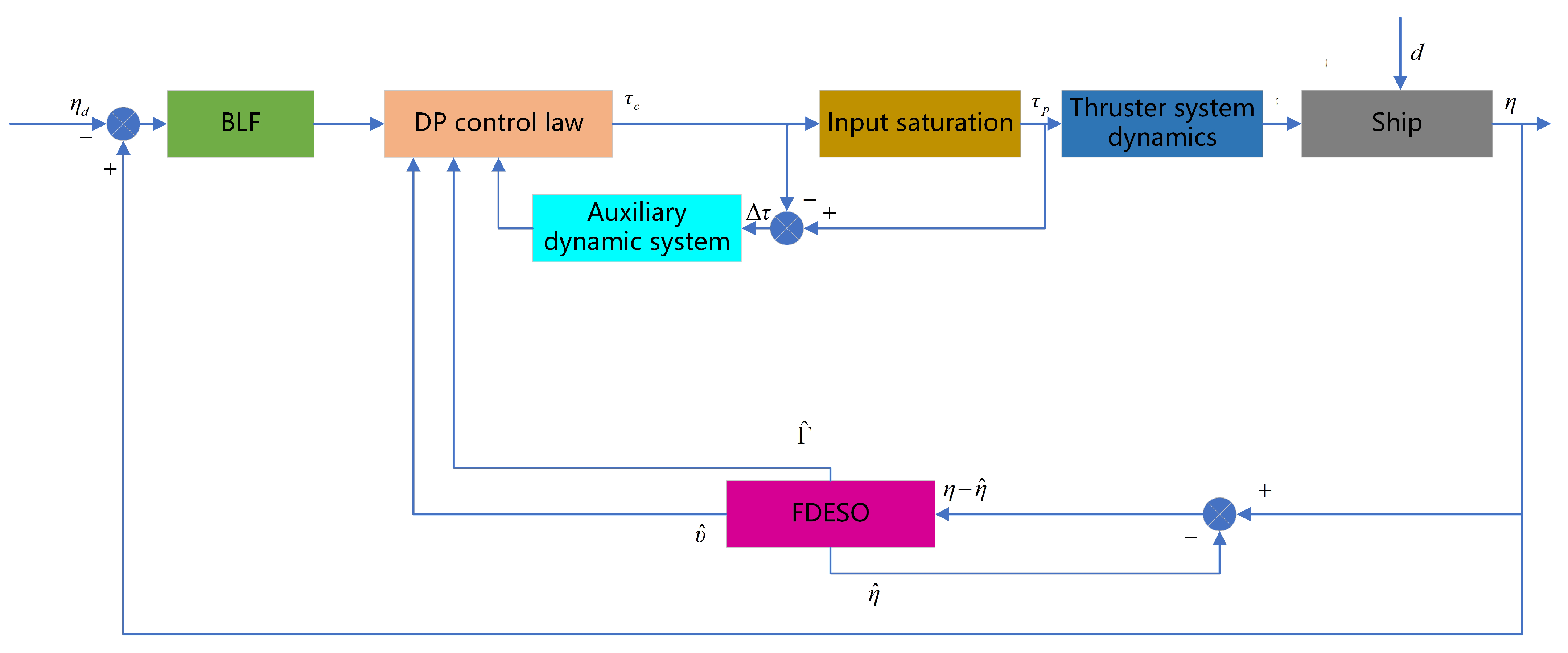
Based on the above, the problems of ship operating position limitation, unmeasurable ship speed, unknown time-varying disturbances, unknown dynamics and input saturation are simultaneously handled in this paper. The ship position is always within the dynamic positioning operation range by introducing the BLF to limit the ship position error. A FDESO is used to estimate the ship’s unmeasurable velocity as well as the set total disturbance, which consists of unknown time-varying disturbances and unknown dynamics. In order to ensure that the generated thrust signal adheres to engineering reality, the controller design takes the thruster system dynamic into account. The input saturation issue is dealt with via a finite-time auxiliary dynamic system. To combat unwanted errors, a robust control term is used. The proposed control law enables the ship position $(x,y)$ and yaw $\psi$ to be reached and keep the anticipated value ${\eta }_d={[x_d,y_d,{\psi }_d]}^T$ with arbitrarily small errors, without exceeding the specified operating area throughout and with all signals in the closed-loop control system consistently and eventually bounded. The major contributions of this paper can be summarized as the following three points.

1.

Throughout the paper, as much as possible, the problems encountered by dynamic positioning systems in complex sea conditions are considered to make them more realistic. For example, there are effects, such as unmeasurable velocity, uncertainty of model parameters, uncertainty of external disturbances, physical characteristics of the thruster system and thruster input saturation. The aforementioned issues are addressed, respectively, using the FDESO, the thruster dynamics equation, and the finite-time auxiliary dynamic system. Among them, FDESO not only estimates the unknown ship speed, but also estimates the total set disturbance caused by unknown model parameters, unknown external disturbance, etc. In addition, a robust control term is introduced in the control strategy to improve the stability of the controlled system.

2.

In the controller design, the ship position is constrained to be within the set range. By introducing the BLF to constrain the ship position error, the ship position is always within the safe working range, which ensures the safety of the ship during operation.

3.

The paper improves the convergence speed of dynamic positioning control method in two ways.

• The use of FDESO significantly improves the convergence speed compared to the high-gain state observer in [46]. According to the detail figure in Figure 4c,d, the convergence speed compared of the presented control scheme is increased by 38.66% comparing with [46].
• The convergence speed is further improved by using a finite-time auxiliary dynamic system to handle the potential input saturation problem.

The rest of this paper is shown below. Section 2 gives the models, assumptions, and lemmas required in the controller design. The design of the FDESO-based dynamic positioning output feedback control rule for position-constrained ships is illustrated, and the system stability is examined in Section 3. In Section 4, lots of comparative simulations are designed, which illustrate the effectiveness and advantages of the control strategy. Section 5 summaries the entire paper.

2. Problem Formulation and Preliminaries

$O-X_0{Y}_0{Z}_0$, which denotes the Earth-fixed inertial frame, and $XYZ$, which denotes the body-fixed frame, are shown in Figure 1.

As is the case for the dynamic positioning control system, the three degrees of freedom of surge, sway and yaw are frequently taken into account in the field of ship motion control. The following diagram illustrates the nonlinear mathematical model of the ship’s dynamic location [47].

$$\begin{array}{cc}\hfill & \dot{\eta }=J\left(\psi \right)\upsilon \hfill \end{array}$$

(1)

$$\begin{array}{cc}\hfill & M\dot{\upsilon }=-D\upsilon +\tau +d\hfill \end{array}$$

(2)

where the ship’s location, expressed in the Earth’s coordinate system as $\eta ={[x,y,\psi ]}^T$, includes the surge position x, sway position y and heading angle $\psi$ of the ship. With surge velocity u, sway velocity v and yaw velocity r being the projections of the velocity vector $\upsilon ={[u,v,r]}^T$ in the three directions of the surge, sway and yaw on the ship body coordinate system, respectively, $\upsilon ={[u,v,r]}^T$ is the ship velocity as it is represented in the body coordinate system. $J\left(\psi \right)\in R^{3\times 3}$ is the rotation matrix to convert the physical quantities between the Earth and body coordinate systems, as follows:

$$\begin{array}{c}\hfill J\left(\psi \right)=\left[\begin{array}{ccc}cos\left(\psi \right)& -sin\left(\psi \right)& 0\\ sin\left(\psi \right)& cos\left(\psi \right)& 0\\ 0& 0& 1\end{array}\right]\end{array}$$

(3)

where $J^{-1}\left(\psi \right)=J^T\left(\psi \right)$, $∥J\left(\psi \right)∥=1$. $M\in R^{3\times 3}$ and $D\in R^{3\times 3}$ are the mass matrix and linear damping matrix of the ship, respectively; $\tau ={[{\tau }_1,{\tau }_2,{\tau }_3]}^T$ is the thrust generated by the thruster, where ${\tau }_1$ is the surge thrust, ${\tau }_2$ is the sway thrust, and ${\tau }_3$ is the yaw thrust. The vector that disturbs the marine ecosystem is $d\in R^3$.

A thruster system dynamics equation is inserted in the controller design as follows to allow the thrust produced by the thruster to make up for the loss of thrust efficiency caused by the actual maritime environment:

$$\begin{array}{c}\hfill \dot{\tau }=-A_{tr}\tau +A_{tr}{\tau }_p\end{array}$$

(4)

where $A_{tr}\in R^{3\times 3}$ is the thruster dynamics matrix, as follows:

$$\begin{array}{c}\hfill A_{tr}=\left[\begin{array}{ccc}\frac{1}{T_{tr1}}& 0& 0\\ 0& \frac{1}{T_{tr2}}& 0\\ 0& 0& \frac{1}{T_{tr3}}\end{array}\right]\end{array}$$

(5)

where $\frac{1}{T_{tr1}}$, $\frac{1}{T_{tr2}}$, and $\frac{1}{T_{tr3}}$ are the equivalent thruster time constants in surge, sway and yaw. For a conventional thruster system, $\frac{1}{T_{tr1}}$ can be approximated by the time constants corresponding to the main propellers; $\frac{1}{T_{tr2}}$ and $\frac{1}{T_{tr3}}$ can be approximated by the time constants to the tunnel and azimuth thrusters. Moreover, it is reasonable to assume that $T_{tr2}\approx T_{tr3}$.

Here, ${\tau }_p\in R^3$ is the thruster system’s control signal restricted because of real-world physical constraints, as in:

$$\begin{array}{c}\hfill {\tau }_{pi}=sat\left({\tau }_{ci}\right)=\left\{\begin{array}{cc}sig\left({\tau }_{ci}\right){\tau }_{Mi}& \left|{\tau }_{ci}\right|\ge {\tau }_{Mi}\\ {\tau }_{ci}& \left|{\tau }_{ci}\right|<{\tau }_{Mi}\end{array},i=1,2,3\right.\end{array}$$

(6)

where ${\tau }_{Mi}>0$ is the maximum thrust value that the thruster can generate, and ${\tau }_c={[{\tau }_{c1},{\tau }_{c2},{\tau }_{c3}]}^T$ is the control signal generated by the designed control strategy. The difference between the restricted control signal ${\tau }_p$ and the unrestrained control signal ${\tau }_c$ is known as $\Delta \tau ={\tau }_p-{\tau }_c$.

Assumption 1.

1. 

The ship model parameter matrices M and D are unknown.

2. 

The ship speed vector $\upsilon ={[u,v,r]}^T$ is unmeasurable.

3. 

The marine environmental disturbance vector $d\in R^3$ is bounded and unknown time-variant; there exists a positive constant $d^{*}>0$ that satisfies

$$\begin{array}{c}\hfill ∥d∥\le d^{*}<\infty \end{array}$$

(7)

Remark 1.

First, the operational circumstances and environment have an impact on the ship. Additionally, the ship is exposed to unidentified time-variant disturbances, which cause the ship model matrices M and D to change. Secondly, most ships’ velocities are not measurable, leading to difficulties in their application in controller design. In addition, the disturbance vector acting on the ship is unknown time-varying and bounded because the ocean environment is constantly changing but energy-limited. Assumption 1 holds.

Since the ship model parameter matrices M and D ingest, we define $M=M_0+\Delta M$ and $D=D_0+\Delta D$, where $M_0$, $D_0$ are nominal values and $\Delta M$, $\Delta D$ are uncertainty terms. Therefore, (2) can be expressed as

$$\begin{array}{c}\hfill M_0\dot{\upsilon }=-D_0\upsilon +\tau +d+\Delta \end{array}$$

(8)

where

$$\begin{array}{c}\hfill M_0=\left[\begin{array}{ccc}{m}_{11}& 0& 0\\ 0& m_{22}& 0\\ 0& 0& m_{33}\end{array}\right]\end{array}$$

(9)

$$\begin{array}{c}\hfill D_0=\left[\begin{array}{ccc}{d}_{11}& 0& 0\\ 0& d_{22}& d_{23}\\ 0& d_{32}& d_{33}\end{array}\right]\end{array}$$

(10)

$$\begin{array}{c}\hfill \Delta =-\Delta M\dot{\upsilon }-\Delta D\upsilon \end{array}$$

(11)

is a composite uncertainty term that includes the model mass matrix and the linear damping matrix ingestion information; $m_{11}$, $m_{22}$, $m_{33}$, $d_{11}$, $d_{22}$, $d_{23}$, $d_{32}$ and $d_{33}$ are all ship model parameters, which will be given later.

Lemma 1

([48,49]). Consider the following system:

$$\begin{array}{c}\hfill \left\{\begin{array}{c}{\dot{z}}_1=z_2-k_{1}si{g}^{{\varsigma }_1}\left(z_1\right)-{\kappa }_{1}si{g}^{{\pi }_1}\left(z_1\right)\hfill \\ {\dot{z}}_2=z_3-k_{2}si{g}^{{\varsigma }_2}\left(z_1\right)-{\kappa }_{2}si{g}^{{\pi }_2}\left(z_1\right)\hfill \\ ⋮\hfill \\ {\dot{z}}_{n-1}=z_n-k_{n-1}si{g}^{{\varsigma }_{n-1}}\left(z_1\right)-{\kappa }_{n-1}si{g}^{{\pi }_{n-1}}\left(z_1\right)\hfill \\ {\dot{z}}_n=-k_{n}si{g}^{{\varsigma }_n}\left(z_1\right)-{\kappa }_{n}si{g}^{{\pi }_n}\left(z_1\right)\hfill \end{array}\right.\end{array}$$

(12)

where $0<{\varsigma }_i<1$, ${\pi }_i>1$ ($i=1,2,\cdots ,n$) and satisfies ${\varsigma }_i=i\varsigma -(i-1)$, ${\pi }_i=i\pi -(i-1)$ ($i=1,2,\cdots ,n$), where $1-{\ell }_1<\varsigma <1$, $1<\pi <1+{\ell }_2$, and ${\ell }_1$, ${\ell }_2$ are sufficiently small positive constants. The matrices formed by the observer gains $k_i$, ${\kappa }_i$ ($i=1,2,\cdots ,n$):

$$\begin{array}{cc}\hfill & A_1=\left[\begin{array}{ccccc}-k_1& 1& 0& \cdots & 0\\ -k_2& 0& 1& \cdots & 0\\ ⋮& & & & \\ -k_{n-1}& 0& 0& \cdots & 1\\ -k_n& 0& 0& \cdots & 0\end{array}\right]\hfill \end{array}$$

(13)

$$\begin{array}{cc}\hfill & A_2=\left[\begin{array}{ccccc}-{\kappa }_1& 1& 0& \cdots & 0\\ -{\kappa }_2& 0& 1& \cdots & 0\\ ⋮& & & & \\ -{\kappa }_{n-1}& 0& 0& \cdots & 1\\ -{\kappa }_n& 0& 0& \cdots & 0\end{array}\right]\hfill \end{array}$$

(14)

are Hurwitz matrices. Then, the system (12) is stable at fixed time and is stable for a time T:

$$\begin{array}{c}\hfill T\le \frac{{{\lambda }_{max}}^{1-\varsigma }\left(P_1\right)}{r_1(1-\varsigma )}+\frac{1}{r_2(\pi -1){{\chi }_0}^{\pi -1}}\end{array}$$

(15)

where $r_1=\frac{{\lambda }_{min}\left(Q_1\right)}{{\lambda }_{max}\left(P_1\right)}$, $r_2=\frac{{\lambda }_{min}\left(Q_2\right)}{{\lambda }_{max}\left(P_2\right)}$, $0<{\chi }_0<{\lambda }_{min}\left(P_2\right)$, and $P_1$, $P_2$, $Q_1$, $Q_2$ are positive definite non-singular matrices and satisfy $P_1{A}_1+{A_1}^T{P}_1=-Q_1$, $P_2{A}_2+{A_2}^T{P}_2=-Q_2$.

Lemma 2

([50]). For a positive definite continuous Lyapunov function $V(x,t)$, the independent variable is defined on $U_1\in R^n$. For the following form:

$$\begin{array}{c}\hfill \dot{V}(x,t)\le -c_1{V}^{\alpha }(x,t)+c_{2}V(x,t),\forall x\in U_1\backslash \left\{0\right\}\end{array}$$

(16)

where $c_1>0$, $c_2>0$, and $0<\alpha <1$, then the system is finite-time stable.

Lemma 3

([51]). For any positive constant $k_{bi}$ ($i=1,2,\dots ,n$), let $S_i:=\{z_i\in R\left|\left|z_i\right|<k_{bi}\right.\}\subset R$ ($i=1,2,\dots ,n$), where $z={[z_1,z_2,\cdots ,z_n]}^T$ ($i=1,2,\dots ,n$), and $N:=R^l\times S_i\subset R^{l+1}$ is an open set, consider the following system:

$$\begin{array}{c}\hfill \dot{x}=f(t,x)\end{array}$$

(17)

where $x={[w^T,z_i]}^T\in N$ is the state vector of the system, and the function $f:R_{+}\times N\to R^{l+1}$ is segmentally continuous with respect to the variable t and satisfies the local Lipschitz condition on $R_{+}\times N$. Suppose there exists a continuously derivable positive definite function $U:R^l\to R_{+}$ and $V_i:z_i\to R_{+}$ ($i=1,2,\dots ,n$) satisfying when $\left|z_i\right|<k_{bi}$, there is

$$\begin{array}{cc}\hfill & V_i\left(z_i\right)\to \infty \hfill \end{array}$$

(18)

$$\begin{array}{cc}\hfill & {\delta }_1\left(∥w∥\right)\le U\left(w\right)\le {\delta }_2\left(∥w∥\right)\hfill \end{array}$$

(19)

where ${\delta }_1$, ${\delta }_2$ are $K_{\infty }$ functions. Let $V\left(x\right):={\displaystyle \sum _{i=1}^n}{V}_i\left(z_i\right)+U\left(w\right)$ and $z_i\left(0\right)\in S_i$. If

$$\begin{array}{c}\hfill \dot{V}=\frac{\partial V}{\partial x}\le -\mu V+\lambda \end{array}$$

(20)

where $x\in N$, and μ and λ are positive constants, then $-k_{bi}<z_i\left(t\right)<k_{bi}$ is satisfied for any $t\ge 0$.

Establishing a reliable nonlinear output feedback dynamic positioning control system based on a BLF is the control goal of this study when some of the model parameters, velocity information and external disturbances are unknown, and there are positional limits on the ship. The proposed control law enables the ship position $(x,y)$ and heading angle $\psi$ to be reached and kept at the expected value ${\eta }_d={[x_d,y_d,{\psi }_d]}^T$ with arbitrarily small errors, and all signals in the closed-loop control system are consistent and eventually bounded.

3. Robust Output Feedback Control Design and System Stability Analysis

During dynamic positioning operations, it is often necessary to delineate a certain working area for each ship for safety reasons to prevent accidents, such as collisions, groundings and ship damage. Therefore, a ship dynamic positioning output feedback control law with position constraint is proposed in this section. Firstly, the unknown ship speed and set total disturbance are estimated by an FDESO and used in the subsequent controller design. Secondly, a BLF is introduced to constrain the ship position. A finite-time auxiliary dynamic system is then used to handle the input saturation problem. In addition, robust control term is used to tackle undesirable errors. The ship dynamic positioning schematic is depicted in Figure 2.

3.1. Design of FDESO

In order to satisfy the condition for the use of FDESO, the ship model depicted in (1) and (2) are transformed and following is the definition of the auxiliary variable.

$$\begin{array}{c}\hfill \zeta =J\left(\psi \right)\upsilon \end{array}$$

(21)

where, $\zeta ={[{\zeta }_1,{\zeta }_2,{\zeta }_3]}^T$.

According to (1) and (21), one can see that

$$\begin{array}{c}\hfill \dot{\eta }=\zeta \end{array}$$

(22)

According to (8) and (21) it is known that

$$\begin{array}{cc}\hfill \dot{\zeta }=& \dot{J}\left(\psi \right)\upsilon +J\left(\psi \right)\dot{\upsilon }\hfill \\ \hfill =& J\left(\psi \right)S\left(r\right)\upsilon +J\left(\psi \right)(-{M_0}^{-1}{D}_0\upsilon +{M_0}^{-1}\tau +{M_0}^{-1}d+{M_0}^{-1}\Delta )\hfill \\ \hfill =& J\left(\psi \right){M_0}^{-1}\tau +J\left(\psi \right)S\left(r\right)\upsilon -J\left(\psi \right){M_0}^{-1}{D}_0\upsilon +J\left(\psi \right){M_0}^{-1}d+J\left(\psi \right){M_0}^{-1}\Delta \hfill \end{array}$$

(23)

where $S\left(r\right)=\left[\begin{array}{ccc}0& -r& 0\\ r& 0& 0\\ 0& 0& 0\end{array}\right]$.

Define the total set disturbance $\Gamma \in R^3$ as depicted below:

$$\begin{array}{cc}\hfill \Gamma =& J\left(\psi \right)S\left(r\right)\upsilon -J\left(\psi \right){M_0}^{-1}{D}_0\upsilon +J\left(\psi \right){M_0}^{-1}d+J\left(\psi \right){M_0}^{-1}\Delta .\hfill \end{array}$$

(24)

Assumption 2.

The set total disturbance Γ satisfies $∥\dot{\Gamma }∥\le {\Gamma }_1$, where ${\Gamma }_1$ is a known bounded constant.

Therefore, according to (22)–(24), the mathematical model of ship dynamic positioning (1) and (2) is rewritten in the following form:

$$\begin{array}{cc}\hfill & \dot{\eta }=\zeta \hfill \end{array}$$

(25)

$$\begin{array}{cc}\hfill & \dot{\zeta }=J\left(\psi \right){M_0}^{-1}\tau +\Gamma .\hfill \end{array}$$

(26)

Since the designed control law requires ship speed information, and to compensate for the set total disturbance formed by unmodeled parameters and external environmental disturbances, a FDESO is designed as depicted below:

$$\begin{array}{c}\hfill \left\{\begin{array}{cc}\dot{\widehat{\eta }}=\hfill & \widehat{\zeta }+{\kappa }_{o,1}si{g}^{{\alpha }_{o,1}}(\eta -\widehat{\eta })+{\epsilon }_{o,1}si{g}^{{\beta }_{o,1}}(\eta -\widehat{\eta })\\ \dot{\widehat{\zeta }}=\hfill & J\left(\psi \right){M_0}^{-1}\tau +\widehat{\Gamma }+{\kappa }_{o,2}si{g}^{{\alpha }_{o,2}}(\eta -\widehat{\eta })+{\epsilon }_{o,2}si{g}^{{\beta }_{o,2}}(\eta -\widehat{\eta })\\ \dot{\widehat{\Gamma }}=\hfill & {\kappa }_{o,3}si{g}^{{\alpha }_{o,3}}(\eta -\widehat{\eta })+{\epsilon }_{o,3}si{g}^{{\beta }_{o,3}}(\eta -\widehat{\eta })+Xsig(\eta -\widehat{\eta })\end{array}\right.\end{array}$$

(27)

where $\widehat{\eta }$, $\widehat{\zeta }$ and $\widehat{\Gamma }$ are the estimates of $\eta$, $\zeta$ and $\Gamma$, respectively. The parameter values satisfy $0<{\alpha }_{o,i}<1$, ${\beta }_{o,i}>1$ ($i=1,2,\cdots ,n$), and satisfy ${\alpha }_{o.i}=i{\alpha }_o-(i-1)$, ${\beta }_{o.i}=i{\beta }_o-(i-1)$, $1-\overline{\alpha }<{\alpha }_o<1$, $1<{\beta }_0<1+\overline{\beta }$, where $\overline{\alpha }$, $\overline{\beta }$ are both sufficiently small positive constants, $X>{\Gamma }_1$. The matrix consisting of the gain ${\kappa }_{o,i}$, ${\epsilon }_{o,i}$ ($i=1,2,3$) of the observer

$$\begin{array}{cc}\hfill & A_{o,1}=\left[\begin{array}{ccc}-{\kappa }_{o,1}& 1& 0\\ -{\kappa }_{o,2}& 0& 1\\ -{\kappa }_{o,3}& 0& 0\end{array}\right]\hfill \end{array}$$

(28)

$$\begin{array}{cc}\hfill & A_{o,2}=\left[\begin{array}{ccc}-{\epsilon }_{o,1}& 1& 0\\ -{\epsilon }_{o,2}& 0& 1\\ -{\epsilon }_{o,3}& 0& 0\end{array}\right]\hfill \end{array}$$

(29)

are all Hurwitz matrices.

Theorem 1.

The designed FDESO (27) can estimate the ship position η, auxiliary variables ζ and set total disturbance Γ under the conditions that satisfy Assumption 1 and Assumption 2, and the estimation error can converge to 0 in fixed time. The convergence time $T_o$ satisfies:

$$\begin{array}{c}\hfill T_o\le \frac{{{\lambda }_{max}}^{1-{\alpha }_o}\left(P_1\right)}{r_{o1}(1-{\alpha }_o)}+\frac{1}{r_{o2}({\beta }_o-1){\chi }^{{\beta }_o-1}}\end{array}$$

(30)

where $r_{o1}=\frac{{\lambda }_{min}\left(Q_1\right)}{{\lambda }_{max}\left(P_1\right)}$, $r_{o2}=\frac{{\lambda }_{min}\left(Q_2\right)}{{\lambda }_{max}\left(P_2\right)}$, $0<\chi <{\lambda }_{min}\left(P_2\right)$, and where $P_1$, $P_2$, $Q_1$ and $Q_2$ are all positive definite non-singular matrices and satisfy $P_1{A}_1+{A_1}^T{P}_1=-Q_1$, $P_2{A}_2+{A_2}^T{P}_2=-Q_2$.

Proof of Theorem 1. 

Define the estimation error of the FDESO:

$$\begin{array}{c}\hfill \left\{\begin{array}{c}{e}_{o,1}=\eta -\widehat{\eta }\\ e_{o,2}=\zeta -\widehat{\zeta }\\ e_{o,3}=\Gamma -\widehat{\Gamma .}\end{array}\right.\end{array}$$

(31)

According to (25)–(27), the derivative of (31) is obtained

$$\begin{array}{c}\hfill \left\{\begin{array}{cc}{\dot{e}}_{o,1}=\hfill & e_{o,2}-{\kappa }_{o,1}si{g}^{{\alpha }_{o,1}}\left(e_{o,1}\right)-{\epsilon }_{o,1}si{g}^{{\beta }_{o,1}}\left(e_{o,1}\right)\hfill \\ {\dot{e}}_{o,2}=\hfill & e_{o,3}-{\kappa }_{o,2}si{g}^{{\alpha }_{o,2}}\left(e_{o,1}\right)-{\epsilon }_{o,2}si{g}^{{\beta }_{o,2}}\left(e_{o,1}\right)\hfill \\ {\dot{e}}_{o,3}=\hfill & \dot{\Gamma }-{\kappa }_{o,3}si{g}^{{\alpha }_{o,3}}\left(e_{o,1}\right)-{\epsilon }_{o,3}si{g}^{{\beta }_{o,3}}\left(e_{o,1}\right)-Xsig\left(e_{o,1}\right).\hfill \end{array}\right.\end{array}$$

(32)

Decompose ${\dot{e}}_{o,3}$ in (32) into the following form:

$$\begin{array}{cc}\hfill & {\dot{e}}_{o,3,1}=-{\kappa }_{o,3}si{g}^{{\alpha }_{o,3}}\left(e_{o,1}\right)-{\epsilon }_{o,3}si{g}^{{\beta }_{o,3}}\left(e_{o,1}\right)\hfill \end{array}$$

(33)

$$\begin{array}{cc}\hfill & {\dot{e}}_{o,3,2}=\dot{\Gamma }-Xsig\left(e_{o,1}\right)\hfill \end{array}$$

(34)

where

$$\begin{array}{c}\hfill {\dot{e}}_{o,3}={\dot{e}}_{o,3,1}+{\dot{e}}_{o,3,2}.\end{array}$$

(35)

Combining ${\dot{e}}_{o,1}$, ${\dot{e}}_{o,2}$ in (32) with (33), it is obtained that

$$\begin{array}{c}\hfill \left\{\begin{array}{c}{\dot{e}}_{o,1}=e_{o,2}-{\kappa }_{o,1}si{g}^{{\alpha }_{o,1}}\left(e_{o,1}\right)-{\epsilon }_{o,1}si{g}^{{\beta }_{o,1}}\left(e_{o,1}\right)\\ {\dot{e}}_{o,2}=e_{o,3}-{\kappa }_{o,2}si{g}^{{\alpha }_{o,2}}\left(e_{o,1}\right)-{\epsilon }_{o,2}si{g}^{{\beta }_{o,2}}\left(e_{o,1}\right)\\ {\dot{e}}_{o,3,1}=-{\kappa }_{o,3}si{g}^{{\alpha }_{o,3}}\left(e_{o,1}\right)-{\epsilon }_{o,3}si{g}^{{\beta }_{o,3}}\left(e_{o,1}\right).\end{array}\right.\end{array}$$

(36)

According to Lemma 1, the system (36) converges to 0 in a fixed time, which means that the observer estimation errors $e_{o,1}$, $e_{o,2}$ and $e_{o,3}$ converge to 0 in a fixed time. and the convergence time $T_o$ satisfies (30). For (34), it follows from [48,49,50] that $e_{o,3,2}\equiv 0$ when $t>T_o$. Therefore, at $t>T_o$, $e_o={[e_{o,1},e_{o,2},e_{o,3}]}^T$ converges to 0. Theorem 1 is proved. □

Thus, at steady state, one can conclude that

$$\begin{array}{cc}\hfill & \eta =\widehat{\eta }\hfill \end{array}$$

(37)

$$\begin{array}{cc}\hfill & \zeta =\widehat{\zeta }\hfill \end{array}$$

(38)

$$\begin{array}{cc}\hfill & \Gamma =\widehat{\Gamma .}\hfill \end{array}$$

(39)

According to (21) and $J^{-1}\left(\psi \right)=J^T\left(\psi \right)$, it follows that

$$\begin{array}{c}\hfill \left\{\begin{array}{c}\upsilon =J^T\left(\psi \right)\zeta \\ \widehat{\upsilon }=J^T\left(\psi \right)\widehat{\zeta .}\end{array}\right.\end{array}$$

(40)

From (38), (40), it is clear that

$$\begin{array}{cc}\hfill \widehat{\upsilon }-\upsilon & =J^T\left(\psi \right)\widehat{\zeta }-J^T\left(\psi \right)\zeta \hfill \\ \hfill & =J^T\left(\psi \right)(\widehat{\zeta }-\zeta )\hfill \\ \hfill & =0.\hfill \end{array}$$

(41)

Therefore, $\upsilon =\widehat{\upsilon }$ holds.

3.2. Design of Robust Output Feedback Control for Dynamic Positioning Considering Position Constraint

The design coordinate transformation is shown below with the velocity measurable:

$$\begin{array}{cc}\hfill & S_1=\eta -{\eta }_d\hfill \end{array}$$

(42)

$$\begin{array}{cc}\hfill & S_2=\upsilon -{\alpha }_1\hfill \end{array}$$

(43)

$$\begin{array}{cc}\hfill & S_3=\tau -{\beta }_1\hfill \end{array}$$

(44)

where ${\eta }_d={[x_d,y_d,{\psi }_d]}^T$ denotes the desired position and heading of the ship, and both ${\alpha }_1\in R^3$ and ${\beta }_1\in R^3$ are intermediate control function vectors, which will be designed later.

According to (1), the derivative of (42) is

$$\begin{array}{c}\hfill {\dot{S}}_1=J\left(\psi \right)\upsilon .\end{array}$$

(45)

Due to the need to constrain the position error $S_1\in R^3$, the BLF $V_1$ is established for the system (45) as

$$\begin{array}{c}\hfill V_1=\frac{1}{2}ln\frac{{K_B}^T{K}_B}{{K_B}^T{K}_B-{S_1}^T{S}_1}\end{array}$$

(46)

where $K_B\in R^3$ is a vector of constant value of ship position error constraint.

Derive (46) from (43), (45)

$$\begin{array}{cc}\hfill {\dot{V}}_1& =\frac{1}{2}·\frac{{K_B}^T{K}_B-{S_1}^T{S}_1}{{K_B}^T{K}_B}·\frac{-{K_B}^T{K}_B(-2{S_1}^T{\dot{S}}_1)}{{({K_B}^T{K}_B-{S_1}^T{S}_1)}^2}\hfill \\ \hfill & =\frac{{S_1}^T{\dot{S}}_1}{{K_B}^T{K}_B-{S_1}^T{S}_1}\hfill \\ \hfill & =\frac{{S_1}^{T}J\left(\psi \right)(S_2+{\alpha }_1)}{{K_B}^T{K}_B-{S_1}^T{S}_1}.\hfill \end{array}$$

(47)

Therefore, the intermediate control function vector ${\alpha }_1\in R^3$ is set to

$$\begin{array}{c}\hfill {\alpha }_1=-({K_B}^T{K}_B-{S_1}^T{S}_1)J^T\left(\psi \right)K_1{S}_1\end{array}$$

(48)

where $K_1={K_1}^T\in R^{3\times 3}$ is the positive definite matrix of the design.

Substituting (48) into (47), the collation gives

$$\begin{array}{cc}\hfill {\dot{V}}_1& =\frac{{S_1}^{T}J\left(\psi \right)S_2+{S_1}^{T}J\left(\psi \right){\alpha }_1}{{K_B}^T{K}_B-{S_1}^T{S}_1}\hfill \\ \hfill & =\frac{{S_1}^{T}J\left(\psi \right)S_2-{S_1}^{T}J\left(\psi \right)({K_B}^T{K}_B-{S_1}^T{S}_1)J^T\left(\psi \right)K_1{S}_1}{{K_B}^T{K}_B-{S_1}^T{S}_1}\hfill \\ \hfill & =-{S_1}^T{K}_1{S}_1+\frac{{S_1}^{T}J\left(\psi \right)S_2}{{K_B}^T{K}_B-{S_1}^T{S}_1}.\hfill \end{array}$$

(49)

According to (21), (26), it can be obtained

$$\begin{array}{cc}\hfill & \frac{d\left[J\right(\psi \left)\upsilon \right]}{dt}=J\left(\psi \right){M_0}^{-1}\tau +\Gamma \hfill \\ \hfill & J\left(\psi \right)S\left(r\right)\upsilon +J\left(\psi \right)\dot{\upsilon }=J\left(\psi \right){M_0}^{-1}\tau +\Gamma \hfill \\ \hfill & J\left(\psi \right)\dot{\upsilon }=J\left(\psi \right){M_0}^{-1}\tau -J\left(\psi \right)S\left(r\right)\upsilon +\Gamma \hfill \\ \hfill & M_0\dot{\upsilon }=\tau -M_{0}S\left(r\right)\upsilon +M_0{J}^T\left(\psi \right)\Gamma .\hfill \end{array}$$

(50)

According to (50), the derivative of (43) is

$$\begin{array}{cc}\hfill M_0{\dot{S}}_2& =M_0\dot{\upsilon }-M_0{\dot{\alpha }}_1\hfill \\ \hfill & =\tau -M_{0}S\left(r\right)\upsilon +M_0{J}^T\left(\psi \right)\Gamma -M_0{\dot{\alpha }}_1.\hfill \end{array}$$

(51)

Establish the Lyapunov function $V_2$ for the system (45), (50) as

$$\begin{array}{c}\hfill V_2=V_1+\frac{1}{2}{S_2}^T{M}_0{S}_2.\end{array}$$

(52)

Derive (52) from (49), (51)

$$\begin{array}{cc}\hfill {\dot{V}}_2=& {\dot{V}}_1+{S_2}^T{M}_0{\dot{S}}_2\hfill \\ \hfill =& -{S_1}^T{K}_1{S}_1+\frac{{S_1}^{T}J\left(\psi \right)S_2}{{K_B}^T{K}_B-{S_1}^T{S}_1}+{S_2}^T(\tau -M_{0}S\left(r\right)\upsilon +M_0{J}^T\left(\psi \right)\Gamma -M_0{\dot{\alpha }}_1).\hfill \end{array}$$

(53)

Define the intermediate control function vector ${\beta }_1\in R^3$ as

$$\begin{array}{cc}\hfill {\beta }_1=& -K_2{S}_2-\frac{J^T\left(\psi \right)S_1}{{K_B}^T{K}_B-{S_1}^T{S}_1}+M_{0}S\left(r\right)\upsilon -M_0{J}^T\left(\psi \right)\Gamma +M_0{\dot{\alpha }}_1+h_r\hfill \end{array}$$

(54)

where $K_2={K_2}^T\in R^{3\times 3}$ is the positive definite matrix of the design.

In order to make the design of the dynamic positioning controller more accurate, the undesirable errors generated in the design are dealt with as follows:

$$\begin{array}{c}\hfill \delta =c^{*}\end{array}$$

(55)

where $c^{*}$ is the normal number, which is the upper bound of the design process that produces undesirable errors, and $h_r$ is the robust control term, as follows:

$$\begin{array}{cc}\hfill & h_r=-\frac{{\widehat{\delta }}^2{S}_2}{\widehat{\delta }∥S_2∥+\rho }\hfill \end{array}$$

(56)

$$\begin{array}{cc}\hfill & \dot{\widehat{\delta }}={\gamma }_1(∥S_2∥-{\gamma }_2\widehat{\delta }),\widehat{\delta }\left(0\right)>0\hfill \end{array}$$

(57)

where $\widehat{\delta }$ is an estimate of $\delta$, and $\rho$, ${\gamma }_1$ and ${\gamma }_2$ are all design parameters.

Based on (4) and $\Delta \tau ={\tau }_p-{\tau }_c$, the derivative of (44) is

$$\begin{array}{cc}\hfill {A_{tr}}^{-1}{\dot{S}}_3& ={A_{tr}}^{-1}\dot{\tau }-{A_{tr}}^{-1}{\dot{\beta }}_1\hfill \\ \hfill & =-\tau +{\tau }_p-{A_{tr}}^{-1}{\dot{\beta }}_1\hfill \\ \hfill & =-\tau +{\tau }_c+\Delta \tau -{A_{tr}}^{-1}{\dot{\beta }}_1.\hfill \end{array}$$

(58)

Furthermore, to address the issue of thruster input saturation, the illustration that follows introduces an auxiliary dynamic system with finite time:

$$\dot{\xi }=\left\{\begin{array}{cc}-K_{{\xi }_1}\xi -K_{{\xi }_2}{\left|\xi \right|}^{r_0}-\frac{{\displaystyle \sum _{i=1}^3}\left|s_{3,i}\Delta {\tau }_i\right|+0.5K_{{\xi }_3}\Delta {\tau }^T\Delta \tau }{{∥\xi ∥}^2}+K_{{\xi }_3}\Delta \tau \hfill & ∥\xi ∥\ge {\xi }_0\\ 0_{3\times 1}\hfill & ∥\xi ∥<{\xi }_0\end{array}\right.$$

(59)

where $\xi ={[{\xi }_1,{\xi }_2,{\xi }_3]}^T$ is the state vector of the auxiliary dynamic system, $K_{{\xi }_1}$ and $K_{{\xi }_2}$ are positive definite parameter design matrices, $K_{{\xi }_3}$ is a positive parameter, ${\xi }_0$ is a positive constant, and the exponential parameter $r_0$ satisfies $0<r_0<1$.

Theorem 2.

The state vector $\xi ={[{\xi }_1,{\xi }_2,{\xi }_3]}^T$ of the finite-time auxiliary dynamic system (59) can converge to zero in finite time.

Proof of Theorem 2.

A Lyapunov function is created for system (59) as follows:

$$\begin{array}{c}\hfill V_{\xi }=\frac{1}{2}{\xi }^T\xi .\end{array}$$

(60)

When $∥\xi ∥\ge {\xi }_0$, according to (59) and Young’s inequality, the derivative of (60) is

$$\begin{array}{cc}\hfill {\dot{V}}_{\xi }=& {\xi }^T\dot{\xi }\hfill \\ \hfill =& -{\xi }^T{K}_{{\xi }_1}\xi -\sum _{i=1}^3{K}_{{\xi }_2,i}{\left|{\xi }_i\right|}^{r_0+1}-\sum _{i=1}^3\left|s_{3,i}\Delta {\tau }_i\right|-\frac{1}{2}{K}_{{\xi }_3}\Delta {\tau }^T\Delta \tau +K_{{\xi }_3}{\xi }^T\Delta \tau \hfill \\ \hfill \le & -{\lambda }_{min}\left(K_{{\xi }_1}\right){∥\xi ∥}^2-{\lambda }_{min}\left(K_{{\xi }_2}\right){∥\xi ∥}^{r_0+1}-\sum _{i=1}^3\left|s_{3,i}\Delta {\tau }_i\right|+\frac{1}{2}{K}_{{\xi }_3}{\xi }^T\xi \hfill \\ \hfill \le & -2[{\lambda }_{min}\left(K_{{\xi }_1}\right)-\frac{1}{2}{K}_{{\xi }_3}]V_{\xi }-2^{\frac{r_0+1}{2}}{\lambda }_{min}\left(K_{{\xi }_2}\right){V_{\xi }}^{\frac{r_0+1}{2}}.\hfill \end{array}$$

(61)

According to Lemma 2, the state vector $\xi ={[{\xi }_1,{\xi }_2,{\xi }_3]}^T$ converges to 0 in finite time when ${\lambda }_{min}\left(K_{{\xi }_1}\right)>\frac{1}{2}{K}_{{\xi }_3}$. Theorem 2 is proved. □

Further, the dynamic positioning state feedback control law in the case where the state is known is designed as

$$\begin{array}{c}\hfill {{\tau }_c}_0=-K_3{S}_3+\tau +{A_{tr}}^{-1}{\dot{\beta }}_1+K_{\xi }\xi -S_2\end{array}$$

(62)

where $K_3={K_3}^T\in R^{3\times 3}$ is the positive definite matrix of the design.

According to Assumption 1, it is known that some of the required states in the control law (62) are unknown, and the estimates $\widehat{\eta }$, $\widehat{\zeta }$, $\widehat{\Gamma }$ and $\widehat{\upsilon }$ obtained in the FDESO (27), and (40) need to be used instead of the true values $\eta$, $\zeta$, $\Gamma$ and $\upsilon$ in the previous section.

Define the new error vector as follows for the ship dynamic positioning output feedback control system in the case of an unknown state:

$$\begin{array}{cc}\hfill & {\widehat{S}}_1=\widehat{\eta }-{\eta }_d\hfill \end{array}$$

(63)

$$\begin{array}{cc}\hfill & {\widehat{S}}_2=\widehat{\upsilon }-{\widehat{\alpha }}_1\hfill \end{array}$$

(64)

$$\begin{array}{cc}\hfill & {\widehat{S}}_3=\tau -{\widehat{\beta }}_1\hfill \end{array}$$

(65)

where

$$\begin{array}{cc}\hfill {\widehat{\alpha }}_1=& -({K_B}^T{K}_B-{{\widehat{S}}_1}^T{\widehat{S}}_1)J^T\left(\psi \right)K_1{\widehat{S}}_1\hfill \end{array}$$

(66)

$$\begin{array}{cc}\hfill {\widehat{\beta }}_1=& -K_2{\widehat{S}}_2-\frac{J^T\left(\psi \right){\widehat{S}}_1}{{K_B}^T{K}_B-{{\widehat{S}}_1}^T{\widehat{S}}_1}+M_{0}S\left(\widehat{r}\right)\widehat{\upsilon }-M_0{J}^T\left(\psi \right)\widehat{\Gamma }+M_0{\dot{\widehat{\alpha }}}_1+{\widehat{h}}_r\hfill \end{array}$$

(67)

where the estimated value of the robust control term $h_r$ is

$$\begin{array}{cc}\hfill & {\widehat{h}}_r=-\frac{{\widehat{\delta }}^2{\widehat{S}}_2}{\widehat{\delta }∥{\widehat{S}}_2∥+\rho }\hfill \end{array}$$

(68)

$$\begin{array}{cc}\hfill & \dot{\widehat{\delta }}={\gamma }_1(∥{\widehat{S}}_2∥-{\gamma }_2\widehat{\delta }),\widehat{\delta }\left(0\right)>0.\hfill \end{array}$$

(69)

In the state unknown case, the finite-time auxiliary dynamic system changes to (70)

$$\dot{\widehat{\xi }}=\left\{\begin{array}{cc}-K_{{\xi }_1}\widehat{\xi }-K_{{\xi }_2}{\left|\widehat{\xi }\right|}^{r_0}-\frac{{\displaystyle \sum _{i=1}^3}\left|{\widehat{s}}_{3,i}\Delta {\tau }_i\right|+0.5K_{{\xi }_3}\Delta {\tau }^T\Delta \tau }{{∥\widehat{\xi }∥}^2}+K_{{\xi }_3}\Delta \tau \hfill & ∥\widehat{\xi }∥\ge {\xi }_0\\ 0_{3\times 1}\hfill & ∥\widehat{\xi }∥<{\xi }_0.\end{array}\right.$$

(70)

Thus, the dynamic positioning output feedback control strategy in the case of unknown state is designed as

$$\begin{array}{c}\hfill {\tau }_c=-K_3{\widehat{S}}_3+\tau +{A_{tr}}^{-1}{\dot{\widehat{\beta }}}_1+K_{\xi }\widehat{\xi }-{\widehat{S}}_2.\end{array}$$

(71)

From (37)–(39), and (41), it follows that at steady state ($t>T_o$), the estimates $\widehat{\eta }$, $\widehat{\zeta }$, $\widehat{\Gamma }$ and $\widehat{\upsilon }$ of the state vector of the FDESO agree with the true values $\eta$, $\zeta$, $\Gamma$ and $\upsilon$. Therefore, at the steady state ($t>T_o$), there are ${\widehat{S}}_1=S_1$, ${\widehat{S}}_2=S_2$, ${\widehat{S}}_3=S_3$, ${\widehat{\alpha }}_1={\alpha }_1$, ${\widehat{\beta }}_1={\beta }_1$, ${\widehat{h}}_r=h_r$, $\widehat{\xi }=\xi$ and ${\tau }_c={\tau }_{c0}$ hold.

3.3. Proof of Stability

A Lyapunov function is created for the dynamic positioning output feedback system as depicted below:

$$\begin{array}{cc}\hfill V=& \frac{1}{2}ln\frac{{K_B}^T{K}_B}{{K_B}^T{K}_B-{S_1}^T{S}_1}+\frac{1}{2}{S_2}^T{M}_0{S}_2+\frac{1}{2}{S_3}^T{A_{tr}}^{-1}{S}_3+\frac{1}{2}{\xi }^T\xi +\frac{1}{2{\gamma }_1}{\tilde{\delta }}^2\hfill \end{array}$$

(72)

where $\tilde{\delta }=\widehat{\delta }-\delta$.

Performing a deflationary transformation on (72) yields

$$\begin{array}{cc}\hfill V>& \frac{1}{2}·\frac{{S_1}^T{S}_1}{{K_B}^T{K}_B}+\frac{1}{2}{S_2}^T{M}_0{S}_2+\frac{1}{2}{S_3}^T{A_{tr}}^{-1}{S}_3+\frac{1}{2}{\xi }^T\xi +\frac{1}{2{\gamma }_1}{\tilde{\delta }}^2.\hfill \end{array}$$

(73)

Derivation of (72)

$$\begin{array}{c}\hfill \dot{V}=\frac{{S_1}^T{\dot{S}}_1}{{K_B}^T{K}_B-{S_1}^T{S}_1}+{S_2}^T{M}_0{\dot{S}}_2+{S_3}^T{A_{tr}}^{-1}{\dot{S}}_3+{\xi }^T\dot{\xi }+\frac{1}{{\gamma }_1}\tilde{\delta }\dot{\widehat{\delta }}.\end{array}$$

(74)

According to (44), (47), (49), (53), (54) and Young’s inequality, it is known that

$$\begin{array}{cc}\hfill {\dot{V}}_2=& \frac{{S_1}^T{\dot{S}}_1}{{K_B}^T{K}_B-{S_1}^T{S}_1}+{S_2}^T{M}_0{\dot{S}}_2\hfill \\ \hfill =& -{S_1}^T{K}_1{S}_1+\frac{{S_1}^{T}J\left(\psi \right)S_2}{{K_B}^T{K}_B-{S_1}^T{S}_1}+{S_2}^T(\tau -M_{0}S\left(r\right)\upsilon +M_0{J}^T\left(\psi \right)\Gamma -M_0{\dot{\alpha }}_1)\hfill \\ \hfill =& -{S_1}^T{K}_1{S}_1+\frac{{S_1}^{T}J\left(\psi \right)S_2}{{K_B}^T{K}_B-{S_1}^T{S}_1}+{S_2}^T(-K_2{S}_2-\frac{J^T\left(\psi \right)S_1}{{K_B}^T{K}_B-{S_1}^T{S}_1}-{\beta }_1+h_r+\tau )\hfill \\ \hfill =& -{S_1}^T{K}_1{S}_1+\frac{{S_1}^{T}J\left(\psi \right)S_2}{{K_B}^T{K}_B-{S_1}^T{S}_1}+{S_2}^T(-K_2{S}_2-\frac{J^T\left(\psi \right)S_1}{{K_B}^T{K}_B-{S_1}^T{S}_1}+S_3+h_r)\hfill \\ \hfill =& -{S_1}^T{K}_1{S}_1-{S_2}^T{K}_2{S}_2+{S_2}^T{S}_3+{S_2}^T{h}_r\hfill \\ \hfill \le & -{S_1}^T{K}_1{S}_1-{S_2}^T{K}_2{S}_2+\frac{1}{2}{S_2}^T{S}_2+\frac{1}{2}{S_3}^T{S}_3+{S_2}^T{h}_r.\hfill \end{array}$$

(75)

Using (58), (71), (72), ${\widehat{S}}_2=S_2$, ${\widehat{S}}_3=S_3$, ${\widehat{\beta }}_1={\beta }_1$, $\widehat{\xi }=\xi$ and Young’s inequality, it follows that

$$\begin{array}{cc}\hfill {S_3}^T{A_{tr}}^{-1}{\dot{S}}_3=& {S_3}^T(-\tau +{\tau }_c+\Delta \tau -{A_{tr}}^{-1}{\dot{\beta }}_1)\hfill \\ \hfill =& {S_3}^T(-K_3{\widehat{S}}_3+{A_{tr}}^{-1}{\dot{\widehat{\beta }}}_1+K_{\xi }\widehat{\xi }-{\widehat{S}}_2+\Delta \tau -{A_{tr}}^{-1}{\dot{\beta }}_1)\hfill \\ \hfill =& -{S_3}^T{K}_3{S}_3+{S_3}^T{K}_{\xi }\xi -{S_3}^T{S}_2+{S_3}^T\Delta \tau \hfill \\ \hfill \le & -{S_3}^T{K}_3{S}_3-\frac{1}{2}{S_2}^T{S}_2+\frac{1}{2}{\xi }^T{K_{\xi }}^T{K}_{\xi }\xi +{S_3}^T\Delta \tau .\hfill \end{array}$$

(76)

When $∥\xi ∥\ge {\xi }_0$, according to (61) and Young’s inequality yields

$$\begin{array}{cc}\hfill {\xi }^T\dot{\xi }=& -{\xi }^T{K}_{{\xi }_1}\xi -\sum _{i=1}^3{K}_{{\xi }_2,i}{\left|{\xi }_i\right|}^{r_0+1}-\sum _{i=1}^3\left|s_{3,i}\Delta {\tau }_i\right|-\frac{1}{2}{K}_{{\xi }_3}\Delta {\tau }^T\Delta \tau +K_{{\xi }_3}{\xi }^T\Delta \tau \hfill \\ \hfill \le & -{\xi }^T{K}_{{\xi }_1}\xi -\sum _{i=1}^3{K}_{{\xi }_2,i}{\left|{\xi }_i\right|}^{r_0+1}-\sum _{i=1}^3\left|s_{3,i}\Delta {\tau }_i\right|+\frac{1}{2}{K}_{{\xi }_3}{\xi }^T\xi \hfill \\ \hfill \le & -{\xi }^T{K}_{{\xi }_1}\xi -\sum _{i=1}^3\left|s_{3,i}\Delta {\tau }_i\right|+\frac{1}{2}{K}_{{\xi }_3}{\xi }^T\xi .\hfill \end{array}$$

(77)

When $∥\xi ∥<{\xi }_0$, according to (59) and Young’s inequality obtains

$$\begin{array}{c}\hfill {\xi }^T\dot{\xi }=0\end{array}$$

(78)

$$\begin{array}{cc}\hfill \frac{1}{2}{\xi }^T{K_{\xi }}^T{K}_{\xi }\xi & ={\xi }^T{K_{\xi }}^T{K}_{\xi }\xi -\frac{1}{2}{\xi }^T{K_{\xi }}^T{K}_{\xi }\xi \hfill \\ \hfill & <-\frac{1}{2}{\xi }^T{K_{\xi }}^T{K}_{\xi }\xi +{{\xi }_0}^2∥{K_{\xi }}^T{K}_{\xi }∥\hfill \end{array}$$

(79)

$$\begin{array}{c}\hfill {S_3}^T\Delta \tau \le \frac{1}{2}{S_3}^T{S}_3+\frac{1}{2}{∥\Delta \tau ∥}^2.\end{array}$$

(80)

From (57), it follows that

$$\begin{array}{cc}\hfill \frac{1}{{\gamma }_1}\tilde{\delta }\dot{\widehat{\delta }}& =\frac{1}{{\gamma }_1}\tilde{\delta }{\gamma }_1(∥S_2∥-{\gamma }_2\widehat{\delta })\hfill \\ \hfill & =\tilde{\delta }(∥S_2∥-{\gamma }_2\widehat{\delta })\hfill \\ \hfill & =\tilde{\delta }∥S_2∥-{\gamma }_2\tilde{\delta }\widehat{\delta .}\hfill \end{array}$$

(81)

Further, according to (56) and $\tilde{\delta }=\widehat{\delta }-\delta$, it is known that

$$\begin{array}{cc}\hfill {S_2}^T{h}_r+\tilde{\delta }∥S_2∥& =-\frac{{\widehat{\delta }}^2{S_2}^T{S}_2}{\widehat{\delta }∥S_2∥+\rho }+\tilde{\delta }∥S_2∥\hfill \\ \hfill & \le -\frac{{\widehat{\delta }}^2{S_2}^T{S}_2}{\widehat{\delta }∥S_2∥+\rho }+\widehat{\delta }∥S_2∥\hfill \\ \hfill & \le \rho \frac{\widehat{\delta }∥S_2∥}{\widehat{\delta }∥S_2∥+\rho }\hfill \\ \hfill & \le \rho \hfill \end{array}$$

(82)

$$\begin{array}{cc}\hfill -{\gamma }_2\tilde{\delta }\widehat{\delta }& =-\frac{{\gamma }_2}{2}{\tilde{\delta }}^2-\frac{{\gamma }_2}{2}{\widehat{\delta }}^2+\frac{{\gamma }_2}{2}{(\tilde{\delta }-\widehat{\delta })}^2\hfill \\ \hfill & =-\frac{{\gamma }_2}{2}{\tilde{\delta }}^2-\frac{{\gamma }_2}{2}{\widehat{\delta }}^2+\frac{{\gamma }_2}{2}{(-\delta )}^2\hfill \\ \hfill & \le -\frac{{\gamma }_2}{2}{\tilde{\delta }}^2+\frac{{\gamma }_2}{2}{\delta }^2.\hfill \end{array}$$

(83)

In the case of $∥\xi ∥\ge {\xi }_0$, substituting (75)–(77) and (81)–(83) into (74), it follows that

$$\begin{array}{cc}\hfill \dot{V}\le & -{S_1}^T{K}_1{S}_1-{S_2}^T{K}_2{S}_2-{S_3}^T{K}_3{S}_3+\frac{1}{2}{S_3}^T{S}_3+\frac{1}{2}{\xi }^T{K_{\xi }}^T{K}_{\xi }\xi -{\xi }^T{K}_{{\xi }_1}\xi +\frac{1}{2}{K}_{{\xi }_3}{\xi }^T\xi -\frac{{\gamma }_2}{2}{\tilde{\delta }}^2+\rho +\frac{{\gamma }_2}{2}{\delta }^2.\hfill \end{array}$$

(84)

Organize, obtain

$$\begin{array}{cc}\hfill \dot{V}& \le -{S_1}^T{K}_1{S}_1-{S_2}^T{K}_2{S}_2-{S_3}^T(K_3-\frac{1}{2}{I}_{3\times 3})S_3-{\xi }^T(K_{{\xi }_1}-\frac{1}{2}{K_{\xi }}^T{K}_{\xi }-\frac{1}{2}{K}_{{\xi }_3}{I}_{3\times 3})\xi -\frac{{\gamma }_2}{2}{\tilde{\delta }}^2+\rho +\frac{{\gamma }_2}{2}{\delta }^2\hfill \\ \hfill & \le -2{\mu }_{1}V+C_1\hfill \end{array}$$

(85)

where

$$\begin{array}{cc}\hfill {\mu }_1=& min\{{\lambda }_{min}\left(K_1\right){K_B}^T{K}_B,{\lambda }_{min}\left(K_2{M_0}^{-1}\right),{\lambda }_{min}\left((K_3-\frac{1}{2}{I}_{3\times 3})A_{tr}\right),{\lambda }_{min}(K_{{\xi }_1}-\frac{1}{2}{K_{\xi }}^T{K}_{\xi }-\frac{1}{2}{K}_{{\xi }_3}{I}_{3\times 3}),\frac{{\gamma }_1{\gamma }_2}{2}\}\hfill \end{array}$$

(86)

and

$$\begin{array}{c}\hfill C_1=\frac{{\gamma }_2}{2}{\delta }^2+\rho .\end{array}$$

(87)

The design matrices $K_1$, $K_2$, $K_3$, $K_{\xi }$ and $K_{{\xi }_1}$ need to satisfy the following conditions

$$\begin{array}{cc}\hfill & {\lambda }_{min}\left(K_1\right)>0\hfill \end{array}$$

(88)

$$\begin{array}{cc}\hfill & {\lambda }_{min}\left(K_2\right)>0\hfill \end{array}$$

(89)

$$\begin{array}{cc}\hfill & {\lambda }_{min}\left(K_3\right)>\frac{1}{2}\hfill \end{array}$$

(90)

$$\begin{array}{cc}\hfill & {\lambda }_{min}(K_{{\xi }_1}-\frac{1}{2}{K_{\xi }}^T{K}_{\xi }-\frac{1}{2}{K}_{{\xi }_3}{I}_{3\times 3})>0.\hfill \end{array}$$

(91)

In the case of $∥\xi ∥<{\xi }_0$, substituting (75), (76) and (78)–(83) into (74), it follows that

$$\begin{array}{cc}\hfill \dot{V}\le & -{S_1}^T{K}_1{S}_1-{S_2}^T{K}_2{S}_2-{S_3}^T{K}_3{S}_3+{S_3}^T{S}_3-\frac{1}{2}{\xi }^T{K_{\xi }}^T{K}_{\xi }\xi -\frac{{\gamma }_2}{2}{\tilde{\delta }}^2+{{\xi }_0}^2∥{K_{\xi }}^T{K}_{\xi }∥+\frac{1}{2}{∥\Delta \tau ∥}^2+\frac{{\gamma }_2}{2}{\delta }^2+\rho .\hfill \end{array}$$

(92)

Organize and obtain

$$\begin{array}{cc}\hfill \dot{V}& \le -{S_1}^T{K}_1{S}_1-{S_2}^T{K}_2{S}_2-{S_3}^T(K_3-I_{3\times 3})S_3-\frac{1}{2}{\xi }^T{K_{\xi }}^T{K}_{\xi }\xi -\frac{{\gamma }_2}{2}{\tilde{\delta }}^2+{{\xi }_0}^2∥{K_{\xi }}^T{K}_{\xi }∥+\frac{1}{2}{∥\Delta \tau ∥}^2+\frac{{\gamma }_2}{2}{\delta }^2+\rho \hfill \\ \hfill & \le -2{\mu }_{2}V+C_2\hfill \end{array}$$

(93)

where

$$\begin{array}{cc}\hfill {\mu }_2=& min\{{\lambda }_{min}\left(K_1\right){K_B}^T{K}_B,{\lambda }_{min}\left(K_2{M_0}^{-1}\right),{\lambda }_{min}\left((K_3-I_{3\times 3})A_{tr}\right),{\lambda }_{min}\left({K_{\xi }}^T{K}_{\xi }\right),\frac{{\gamma }_1{\gamma }_2}{2}\}\hfill \end{array}$$

(94)

and

$$\begin{array}{c}\hfill C_2={{\xi }_0}^2∥{K_{\xi }}^T{K}_{\xi }∥+\frac{1}{2}{∥\Delta \tau ∥}^2+\frac{{\gamma }_2}{2}{\delta }^2+\rho .\end{array}$$

(95)

The design matrices $K_1$, $K_2$, $K_3$ and $K_{\xi }$, need to satisfy the following conditions:

$$\begin{array}{cc}\hfill & {\lambda }_{min}\left(K_1\right)>0\hfill \end{array}$$

(96)

$$\begin{array}{cc}\hfill & {\lambda }_{min}\left(K_2\right)>0\hfill \end{array}$$

(97)

$$\begin{array}{cc}\hfill & {\lambda }_{min}\left(K_3\right)>1\hfill \end{array}$$

(98)

$$\begin{array}{cc}\hfill & {\lambda }_{min}\left({K_{\xi }}^T{K}_{\xi }\right)>0.\hfill \end{array}$$

(99)

According to (85) and (93), it follows that

$$\begin{array}{c}\hfill \dot{V}\le -2\mu V+C\end{array}$$

(100)

where $\mu =min\{{\mu }_1,{\mu }_2\}$, $C=max\{C_1,C_2\}$.

Theorem 3.

The dynamic positioning control system with position constraint is able to make the position error vector $S_1$ of the ship (1)–(4) considering the thruster system dynamics always within the bounded set at any moment by choosing the proper design matrix and design parameter values.

Proof of Theorem 3.

According to Lemma 3, when (100) is satisfied, the position error vector $S_1$ satisfies the following condition:

$$\begin{array}{c}\hfill ∥S_1∥\le ∥K_B∥.\end{array}$$

(101)

Therefore, Theorem 3 is proved. □

Theorem 4.

The robust output feedback control system with position constraint for dynamic positioning can enable the ship (1)–(4) considering the thruster system dynamics to arrive and stay on the desired position and heading ${\eta }_d={[x_d,y_d,{\psi }_d]}^T$ within a certain time while satisfying Assumptions 1 and 2. Moreover, by selecting a reasonable design matrix and design parameters, it is possible to make all signals in the whole closed-loop control system consistent and ultimately constrained.

Proof of Theorem 4.

Solving for (100) yields

$$\begin{array}{c}\hfill 0\le V\left(t\right)\le \frac{C}{2\mu }+[V\left(0\right)-\frac{C}{2\mu }]e^{-2\mu t}.\end{array}$$

(102)

According to (102), it is known that the Lyapunov function of the dynamic positioning output feedback system is consistently and eventually bounded. Then, from (72), it is known that $∥S_1∥$, $∥S_2∥$, $∥S_3∥$, $∥\xi ∥$ and $∥\tilde{\delta }∥$ are consistently eventually bounded. Since ${\eta }_d$ is a set constant, it follows from (42) that $\eta$ is bounded. By (48), ${\alpha }_1$ is bounded, and further, by (43), $\upsilon$ is bounded. From (6), ${\tau }_p$ is bounded, and by extension, from (4), $\tau$ is bounded. Therefore, from (44), one knows that ${\beta }_1$ is bounded. Because there is an upper bound for $\Delta \tau$, and $\Delta \tau ={\tau }_p-{\tau }_c$, the control signal ${\tau }_c$ is bounded. According to (55), it is clear that $\delta$ is bounded. From the fact that $\tilde{\delta }=\widehat{\delta }-\delta$ and $∥\tilde{\delta }∥$ are bounded, it follows that $\widehat{\delta }$ is bounded. It is evident from (56) that $h_r$ is bounded. From (7) and (11), it is known that d, $\Delta$ is bounded. Then, according to (24), $\Gamma$ is bounded. Therefore, all signals within the closed-loop control system are bounded. Further, according to (102), it is obtained that

$$\begin{array}{c}\hfill ∥S_1∥\le ∥K_B∥\sqrt{1-e^{\frac{C}{\mu }+2[V\left(0\right)-\frac{C}{2\mu }]e^{-2\mu t}}}.\end{array}$$

(103)

From (97), it is clear that for any positive constant ${\zeta }_{S_1}>∥K_B∥\sqrt{1-e^{\frac{C}{\mu }}}$, there exists a positive constant $T_{S_1}$, when $t>T_{S_1}$, $∥S_1∥\le {\zeta }_{S_1}$. Therefore, $S_1$ converges to a tight set ${\Omega }_{S_1}=\{S_1\in R^3\left|∥S_1∥\le {\zeta }_{S_1}\right.{\zeta }_{S_1}>∥K_B∥\sqrt{1-e^{\frac{C}{\mu }}}\}$. By changing the parameters, this tight set can be made arbitrarily small in a specific amount of time. Therefore, taking into account the dynamics of the thruster system, the ship (1)–(4) is able to reach and maintain the target position and direction in a specific amount of time. Theorem 4 is proved. □

4. Simulation and Analysis

In this section, lots of dynamic positioning simulation experiments are used to demonstrate the efficacy of the suggested control technique. First, to verify that the output feedback control strategy in the speed-unmeasurable case can effectively recover the performance of the state feedback control strategy in the speed-measurable case, the output feedback control law ${\tau }_c$ proposed in (71) and the state feedback control law ${\tau }_{c0}$ proposed in (62) of this paper were subjected to separate dynamic positioning simulation experiments and compared. Secondly, the output feedback control strategy ${\tau }_c$ provided in this paper is contrasted with the output feedback control strategy provided in [46], and then the effectiveness and superiority of introducing the BLF, introducing the FDESO and considering the thruster system dynamics are illustrated. Here, a supply vessel Northern Clipper with dimensions of $76.2$ m in length and $4.591\times {10}^6$ kg in mass is simulated with the nominal model parameters and thruster parameters shown in

Table 1. Parameter of the supply vessel Northern Clipper.

${\mathit{m}}_{11}$	$5.3122\times {10}^6$	${\mathit{m}}_{22}$	$8.2831\times {10}^6$
$m_{33}$	$3.7454\times {10}^9$	$d_{11}$	$5.0242\times {10}^4$
$d_{22}$	$2.7229\times {10}^5$	$d_{23}$	$-4.3933\times {10}^6$
$d_{32}$	$-4.3933\times {10}^6$	$d_{33}$	$4.1894\times {10}^8$
$T_{tr1}$	5	$T_{tr2}$	5
$T_{tr3}$	5

[47]:

The thruster input saturation issue must be taken into account in the intended control strategy due to the physical constraints of the supply vessel thrusters.

Table 2. Thruster input saturation limit values.

	Thrusters	Limits
Surge	${\tau }_{M1}$	$3.76815\times {10}^2$ (kN)
Sway	${\tau }_{M2}$	$6.8072\times {10}^2$ (kN)
Yaw	${\tau }_{M3}$	$7.31\times {10}^3$ (kN)

shows the thruster input saturation limits for the supply ship Northern Clipper.

The unknown time-varying disturbance $d\in R^3$ in the text is set as $d\left(t\right)=J^T\left(\psi \right)b$, where $b\in R^3$ is taken from the first-order Markov process $\dot{b}=-T^{-1}b+\Psi \overline{\omega }$ as the bias force and moment vector, $T\in R^{3\times 3}$ is the time constant matrix, $\overline{\omega }\in R^3$ is the Gaussian white noise vector with mean 0, and $\Psi \in R^{3\times 3}$ is the diagonal matrix of the tuning $\overline{\omega }$. Set the disturbance scene parameters as $b\left(0\right)={[10\mathrm{kN},10\mathrm{kN},10\mathrm{kNm}]}^T$, $T=diag({10}^3,{10}^3,{10}^3)$ and $\Psi =diag(3\times {10}^4,3\times {10}^4,3\times {10}^5)$.

The desired position and heading of the ship are set to ${\eta }_d={[0\mathrm{m},0\mathrm{m},0^{\circ }]}^T$, and the initial values of the initial state of the ship and some of the controller parameters are $\eta \left(0\right)={[20\mathrm{m},20\mathrm{m},10{}^{\circ }]}^T$, $\upsilon \left(0\right)={[0\mathrm{m}/\mathrm{s},0\mathrm{m}/\mathrm{s},0{}^{\circ }/\mathrm{s}]}^T$, $\tau \left(0\right)={[0,0,0]}^T$, $\eta \left(0\right)={[20\mathrm{m},20\mathrm{m},10{}^{\circ }]}^T$, $\widehat{\zeta }\left(0\right)={[0,0,0]}^T$, $\widehat{\Gamma }\left(0\right)={[0,0,0]}^T$, $\widehat{\delta }\left(0\right)=10$, $\xi \left(0\right)={[5\times {10}^4,5\times {10}^4,5\times {10}^4]}^T$. The design parameters are $K_1=diag(0.2,0.2,0.2)$, $K_2=diag(1\times {10}^7,1\times {10}^7,8\times {10}^9)$, $K_3=diag(0.3,0.4,0.4)$, ${\kappa }_{o,1}=5$, ${\kappa }_{o,2}=20$, ${\kappa }_{o,3}=50$, ${\epsilon }_{o,1}=5$, ${\epsilon }_{o,2}=20$, ${\epsilon }_{o,3}=50$, ${\alpha }_{o,1}=0.8$, ${\alpha }_{o,2}=0.6$, ${\alpha }_{o,3}=0.4$, ${\beta }_{o,1}=1.2$, ${\beta }_{o,2}=1.4$, ${\beta }_{o,3}=1.6$, $X=1\times {10}^{-3}$, $K_B={[25,25,100]}^T$, $\rho =1\times {10}^3$, ${\gamma }_1=3\times {10}^2$, ${\gamma }_2=1\times {10}^{-7}$, $K_{{\xi }_1}=diag(5,3,5)$, $K_{{\xi }_2}=diag(2,2,5)$, $K_{{\xi }_3}=0.02$, ${\xi }_0=20$, $r_0=\frac{6}{7}$, $K_{\xi }=(5,5,5)$.

4.1. Performance of Proposed Output Feedback Control Law

To verify the performance of the proposed output feedback control strategy in the case of unmeasurable speed, the output feedback control strategy ${\tau }_c$ in (71) is contrasted with the state feedback control strategy ${\tau }_{c0}$ in (62) in the case of known speed, as shown in Figure 3a–d. To verify the validity of the FDESO, the velocity observation $\widehat{\upsilon }$ and the set total disturbance observation $\widehat{\Gamma }$ are compared with the velocity true value $\upsilon$ and the set total disturbance true value $\Gamma$, respectively, as shown in Figure 3e,f.

Figure 3a,b show that the ship can achieve and maintain the desired location and direction ${\eta }_d={[0\mathrm{m},0\mathrm{m},0^{\circ }]}^T$ within a certain time under both output feedback and state feedback control laws, and the ship’s motion trajectory is within the position error bounded range $-25\mathrm{m}<x<25\mathrm{m}$, $-25\mathrm{m}<y<25\mathrm{m}$. The ship’s velocity u, v and r are shown to be constrained in Figure 3c, and the ship velocity produced by the output feedback control technique is nearly identical to the ship velocity produced by the state feedback. Figure 3d indicates that the signals shift smoothly without abrupt changes, and the actual thrust generated by the thruster is within the thruster input saturation limits shown in Table 2. Additionally, the thrusts produced by the output feedback approach and those produced by the state feedback technique are essentially identical. Therefore, the output feedback control strategy proposed in this paper can effectively recover the performance of the state feedback control strategy. Figure 3e shows that the FDESO can effectively observe the unmeasurable velocity, and Figure 3f indicates that the FDESO can estimate the unknown set of total thrusters. Therefore, the FDESO is effective.

4.2. Comparison with Existing DP Control Law

The dynamic positioning output feedback control strategy ${\tau }_h$ based on the high-gain observer proposed in [46] is compared with the dynamic positioning output feedback control law ${\tau }_c$ based on the FDESO proposed in this paper to show the effectiveness and superiority of introducing BLF and FDESO, taking into account the dynamics of the thruster system. This comparison is shown in Figure 4a–e.

Figure 4a,b indicate that the control strategy proposed in this paper can reach and stay on the desired position and heading ${\eta }_d={[0\mathrm{m},0\mathrm{m},0^{\circ }]}^T$ within a certain time, and the ship’s motion trajectory is within the position error limit $-25\mathrm{m}<x<25\mathrm{m}$, $-25\mathrm{m}<y<25\mathrm{m}$. Additionally, it takes about the same amount of time to get to the desired point as the control method of [46]. Figure 4c,d show that both the FDESO proposed in this paper and the high-gain observer proposed in [46] can effectively estimate the unmeasured velocity, and the estimation speed of the FDESO is faster than that of the high-gain observer. Figure 4e illustrates that the actual thrust produced by the control strategy discussed in this paper and the control strategy in [46] are both within the thruster input saturation limit, but the actual thrust signal produced in this paper changes smoothly without abrupt changes, whereas the actual thrust signal produced in [46] has significant fluctuations at the beginning and clearly abrupt changes. As a result, the control technique provided in this work is more in tune with engineering realities than [46].

4.3. Marine System Simulator Toolbox Simulations

It is necessary to plan the related experiments in order to test the suggested control strategy. However, because of the constraints of current engineering development, conducting actual ship testing to verify the applicability of the offered approach is very challenging. About 99 percent of the control systems that have been devised for ship dynamic positioning control cannot be tested on a real ship. However, this study can be replicated using the MSS toolbox, which is well-known in the area and whose disturbance model and ship model are accepted in that field. A semi-realistic ship and disturbance may be constructed using the MSS toolbox, and the developed control system can be utilized as a substitute for an engineering verification system.

The simulation example is a supply vessel from DP MotionRAO, the essential details of which are presented in

Table 3. Main particulars of the supply vessel in DP_MotionRAO.

Length between perpendiculars	$82.8$ m
Draft	6 m
Breadth	$19.2$ m
Mass	$6.3622\times {10}^6$ kg
Displacement	$6.2070\times {10}^3{\mathrm{m}}^3$

. The MSS toolbox contains the nominal values $M_0$ and $D_0$ of the parameters of its motion mathematical model. Also offered is a simulated comparison with the [46] DP control legislation that is now in place.

In simulations, the sea state four is represented by the Jonswap wave spectrum type, significant wave height of 1.5 m, peak frequency of 0.76 rad/s, and mean wave direction of $({35}^{\circ }/{180}^{\circ })\times \pi$ rad in the northeast frame. The mean wind angle is $({30}^{\circ }/{180}^{\circ })\times \pi$ rad, and the wind speed is 5 m/s. The current direction is $({350}^{\circ }/{180}^{\circ })\times \pi$, and the current speed is 0.1 m/s.

To verify the performance of the proposed output feedback control strategy in the case of unmeasurable speed, the output feedback control strategy ${\tau }_c$ in (71) is compared with the state feedback control strategy ${\tau }_{c0}$ in (62) in the case of known speed, as shown in Figure 5a–d. To verify the validity of the FDESO, the velocity observation $\widehat{\upsilon }$ and the set total disturbance observation $\widehat{\Gamma }$ are compared with the velocity true value $\upsilon$ and the set total disturbance true value $\Gamma$, respectively, as shown in Figure 5e,f.

Figure 5a,b show that the ship can reach and stay on the desired location and orientation ${\eta }_d={[0\mathrm{m},0\mathrm{m},0^{\circ }]}^T$ within a certain time under both output feedback and state feedback control laws, and the ship’s motion trajectory is within the position error bounded range $-25\mathrm{m}<x<25\mathrm{m}$, $-25\mathrm{m}<y<25\mathrm{m}$. Figure 5c shows that the ship velocity u, v and r is bounded, and the ship velocity generated by the output feedback control strategy is basically the same as the ship velocity generated by the state feedback. Figure 5d indicates that the actual thrust generated by the thruster is within the thruster input saturation limits shown in Table 2, and the signals change smoothly without sudden changes. Moreover, the thrusts produced by the output feedback strategy are basically the same as that generated by the state feedback strategy. Therefore, the output feedback control strategy proposed in this paper can effectively recover the performance of the state feedback control strategy. Figure 5e shows that the FDESO can effectively observe the unmeasurable velocity, and Figure 5f indicates that the FDESO can estimate the unknown set of total thrusters. Therefore, the FDESO is effective.

The dynamic positioning output feedback control law ${\tau }_h$ based on the high-gain observer proposed in [46] is compared with the dynamic positioning output feedback control strategy ${\tau }_c$ based on the FDESO proposed in this paper in order to demonstrate the effectiveness and superiority of introducing BLF and FDESO, taking into account the dynamics of the thruster system. This comparison is shown in Figure 6a–e.

Figure 6a,b indicate that the control strategy presented in this paper can reach and stay on the desired location and direction ${\eta }_d={[0\mathrm{m},0\mathrm{m},0^{\circ }]}^T$ within a certain time, and the ship’s motion trajectory is within the position error limit $-25\mathrm{m}<x<25\mathrm{m}$, $-25\mathrm{m}<y<25\mathrm{m}$. In addition, it takes about the same amount of time to get to the desired point as the control method of [46]. Figure 6c,d show that both the FDESO proposed in this paper and the high-gain observer proposed in [46] can effectively estimate the unmeasured velocity, and the estimation speed of the FDESO is faster than that of the high-gain observer. Figure 6e shows that the actual thrust produced by the control strategy discussed in this paper and the control strategy in [46] are both within the thruster input saturation limit, but the actual thrust signal produced in this paper changes smoothly without abrupt changes, whereas the actual thrust signal produced in [46] has significant fluctuations at the beginning and clearly abrupt changes.

In the MMS toolbox, the disturbance model is less energetic than white noise, as can be observed by comparing Figure 3, Figure 4, Figure 5 and Figure 6. Because of this, the ship using the toolbox produces less thruster force to mitigate the disruption than the initial supply ship did. The supply ship model using white noise as the disturbance provides control performance that is equivalent to that produced by the ship model and the semi-realistic disturbance in the MMS toolbox, despite the fact that both are capable of creating the required control effect. As a result, it can be shown that the study’s proposed control strategy is dependable and effective.

5. Conclusions

In this paper, the problems encountered in the actual dynamic positioning operation are considered. For example, there are problems, such as ship operation area limitation, unmeasurable speed, unknown time-varying disturbances, unknown dynamics and input saturation. By introducing the BLF to limit the ship position error, the ship position is always within the dynamic positioning operation range. The ship’s unmeasurable velocity and the set total disturbance consisting of unknown time-varying disturbances and unknown dynamics are estimated by an FDESO. The thruster system dynamics equation is considered in the controller design to make the generated thrust signal conform to the engineering reality. The input saturation issue is dealt with via a finite-time auxiliary dynamic system. To combat unwanted mistakes, one uses the robust control concept. A position-constrained dynamic ship positioning output feedback control rule that takes the dynamics of the thruster system into account is constructed by combining the aforementioned parts. The theoretical analysis section shows that the ship position and heading can eventually be maintained at the expected value and that the ship position remains within the designated operating area throughout. All signals in the designed dynamic positioning output feedback control system are eventually and consistently bounded. The simulation results show that the control law is effective and satisfies the engineering reality.

This paper improves the existing dynamic positioning technique by considering as many problems encountered in complex sea conditions as possible to make it more realistic. This paper also considers the effects of unmeasurable speed, the uncertainty of model parameters, the uncertainty of external disturbances, physical characteristics of the thruster system, and input saturation of the thruster system. In addition, in this paper, the ship position error is constrained by introducing BLF in the controller design so that the ship position is always kept within the safe working range, which ensures the safety of the ship during operation. Finally, this paper speeds up the convergence speed by introducing FDESO and a finite-time auxiliary dynamic system.

Since the ship model, actuation dynamics model and disturbance model used in the design of the controller in this paper deviate from the real physical model, the performance of the designed control law will be lower than expected when applied to the actual dynamic positioning.

The following two elements are included in upcoming work. To first achieve dynamic positioning control under various sea circumstances, the switching control technique is included into the dynamic positioning control. In order to achieve automated berthing control, the dynamic positioning control will also introduce the switching control technique and event triggering mechanism.

References

1. Chae, C.J.; Jung, Y.C. An Analysis on Incident Cases of Dynamic Positioning Vessels. J. Navig. Port Res. 2015, 39, 149–156. [Google Scholar] [CrossRef] [Green Version]
2. Chen, H.; Moan, T.; Verhoeven, H. Effect of DGPS failures on dynamic positioning of mobile drilling units in the North Sea. Accid. Anal. Prev. 2009, 41, 1164–1171. [Google Scholar] [CrossRef]
3. Chen, H.; Moan, T.; Verhoeven, H. DGPS failures on mobile offshore drilling units on the Norwegian Continental Shelf. In Proceedings of the 17th European Safety and Reliability Conference, ESREL 2006, Estoril, Portugal, 18–22 September 2006; pp. 2485–2492. [Google Scholar]
4. Chen, H.; Moan, T.; Verhoeven, H. Barriers to prevent loss of position on DP drilling units on the Norwegian Continental Shelf. In Proceedings of the 17th European Safety and Reliability Conference, ESREL 2006, Estoril, Portugal, 18–22 September 2006; pp. 2477–2484. [Google Scholar]
5. Specht, C. Accuracy and coverage of the modernized Polish Maritime differential GPS system. Adv. Space Res. 2011, 47, 221–228. [Google Scholar] [CrossRef]
6. Specht, C.; Weintrit, A.; Specht, M. A History of Maritime Radio-Navigation Positioning Systems used in Poland. J. Navig. 2016, 69, 468–480. [Google Scholar] [CrossRef] [Green Version]
7. Specht, C.; Pawelski, J.; Smolarek, L.; Specht, M.; Dbrowski, P.S. Assessment of the Positioning Accuracy of DGPS and EGNOS Systems in the Bay of Gdansk using Maritime Dynamic Measurements. J. Navig. 2019, 72, 575–587. [Google Scholar] [CrossRef] [Green Version]
8. Specht, C.; Smolarek, L.; Pawelski, J.; Specht, M.; Dabrowski, P. Polish DGPS System: 1995–2017—Study of Positioning Accuracy. Pol. Marit. Res. 2019, 26, 15–21. [Google Scholar] [CrossRef] [Green Version]
9. Fossen, T.I. Guidance and Control of Ocean Vehicles. Ph.D. Thesis, University of Trondheim, Trondheim, Norway, 1999. [Google Scholar]
10. Balchen, J.G.; Jenssen, N.A.; Sælid, S. Dynamic positioning using Kalman filtering and optimal control theory. In IFAC/IFIP Symposium on Automation in Offshore Oil Field Operation; North-Holland Publishing Company: Amsterdam, The Netherlands, 1976; Volume 183, p. 186. [Google Scholar]
11. Balchen, J.G.; Jenssen, N.A.; Mathisen, E.; Saelid, S. Dynamic positioning of floating vessles based on Kalman filtering and optimal control. In Proceedings of the 1980 19th IEEE Conference on Decision and Control including the Symposium on Adaptive Processes, Albuquerque, NM, USA, 10–12 December 1980; pp. 852–864. [Google Scholar]
12. Grovlen, A.; Fossen, T.I. Nonlinear control of dynamic positioned ships using only position feedback: An observer backstepping approach. In Proceedings of the 35th IEEE Conference on Decision and Control, Kobe, Japan, 13 December 1996; Volume 3, pp. 3388–3393. [Google Scholar]
13. Fossen, T.I.; Grovlen, A. Nonlinear output feedback control of dynamically positioned ships using vectorial observer backstepping. IEEE Trans. Control Syst. Technol. 1998, 6, 121–128. [Google Scholar] [CrossRef]
14. Piekło, A.; Witkowska, A.; Zubowicz, T. Dynamic Positioning Capability Assessment for Ship Design Purposes. Lect. Notes Netw. Syst. 2023, 545, 386–397. [Google Scholar]
15. Mauro, F.; Nabergoj, R. A probabilistic approach for Dynamic Positioning capability and operability predictions. Ocean Eng. 2022, 262, 112250. [Google Scholar] [CrossRef]
16. Martelli, M.; Faggioni, N.; Donnarumma, S. A time-domain methodology to assess the dynamic positioning performances. Ocean Eng. 2022, 247, 110668. [Google Scholar] [CrossRef]
17. Mauro, F.; Prpić-Oršić, J. Determination of a DP operability index for an offshore vessel in early design stage. Ocean Eng. 2020, 195, 106764. [Google Scholar] [CrossRef]
18. Smogeli, O.; Trong, N.; Borhaug, B.; Pivano, L. The next level DP capability analysis. In Proceedings of the Dynamic Positioning Conference, Houston, TX, USA, 15–16 October 2013. [Google Scholar]
19. Do, K.D. Global robust and adaptive output feedback dynamic positioning of surface ships. J. Mar. Sci. Appl. 2011, 10, 325–332. [Google Scholar] [CrossRef]
20. Ma, Y.; Zhu, G.; Li, Z. Error-Driven-Based Nonlinear Feedback Recursive Design for Adaptive NN Trajectory Tracking Control of Surface Ships With Input Saturation. IEEE Intell. Transp. Syst. Mag. 2019, 11, 17–28. [Google Scholar] [CrossRef]
21. Zhang, G.; Huang, C.; Zhang, X.; Tian, B. Robust adaptive control for dynamic positioning ships in the presence of input constraints. J. Mar. Sci. Technol. 2019, 24, 1172–1182. [Google Scholar] [CrossRef]
22. Du, J.; Yang, Y.; Wang, D.; Guo, C. A robust adaptive neural networks controller for maritime dynamic positioning system. Neurocomputing 2013, 110, 128–136. [Google Scholar] [CrossRef]
23. Du, J.; Hu, X.; Krstić, M.; Sun, Y. Robust dynamic positioning of ships with disturbances under input saturation. Automatica 2016, 73, 207–214. [Google Scholar] [CrossRef]
24. Hu, X.; Du, J. Robust nonlinear control design for dynamic positioning of marine vessels with thruster system dynamics. Nonlinear Dyn. 2018, 94, 365–376. [Google Scholar] [CrossRef]
25. Tee, K.P.; Ge, S.S.; Tay, F. Adaptive Control of Electrostatic Microactuators With Bidirectional Drive. IEEE Trans. Control Syst. Technol. 2009, 17, 340–352. [Google Scholar]
26. Tu, F.; Ge, S.S.; Choo, Y.S.; Hang, C.C. Adaptive dynamic positioning control for accommodation vessels with multiple constraints. IET Control Theory Appl. 2017, 11, 329–340. [Google Scholar] [CrossRef]
27. Yin, Z.; He, W.; Yang, C. Tracking control of a marine surface vessel with full-state constraints. Int. J. Syst. Sci. 2017, 48, 535–546. [Google Scholar] [CrossRef] [Green Version]
28. Zheng, Z.; Huang, Y.; Xie, L.; Zhu, B. Adaptive trajectory tracking control of a fully actuated surface vessel with asymmetrically constrained input and output. IEEE Trans. Control Syst. Technol. 2017, 26, 1851–1859. [Google Scholar] [CrossRef]
29. Kong, L.; He, W.; Yang, C.; Li, G.; Zhang, Z. Adaptive fuzzy control for a marine vessel with time-varying constraints. IET Control Theory Appl. 2018, 12, 1448–1455. [Google Scholar] [CrossRef]
30. Qin, H.; Li, C.; Sun, Y.; Li, X.; Du, Y.; Deng, Z. Finite-time trajectory tracking control of unmanned surface vessel with error constraints and input saturations. J. Frankl. Inst. 2020, 357, 11472–11495. [Google Scholar] [CrossRef]
31. Zhang, J.; Yu, S.; Yan, Y.; Wu, D. Fixed-time output feedback sliding mode tracking control of marine surface vessels under actuator faults with disturbance cancellation. Appl. Ocean Res. 2020, 104, 102378. [Google Scholar] [CrossRef]
32. Hao, L.Y.; Yu, Y.; Li, T.S.; Li, H. Quantized Output-Feedback Control for Unmanned Marine Vehicles With Thruster Faults via Sliding-Mode Technique. IEEE Trans. Cybern. 2021, 52, 9363–9376. [Google Scholar] [CrossRef]
33. Zhu, G.; Ma, Y.; Li, Z.; Malekian, R.; Sotelo, M.A. Adaptive Neural Output Feedback Control for MSVs With Predefined Performance. IEEE Trans. Veh. Technol. 2021, 70, 2994–3006. [Google Scholar] [CrossRef]
34. Hu, X.; Zhu, G.; Ma, Y.; Li, Z.; Malekian, R.; Sotelo, M. Event-Triggered Adaptive Fuzzy Setpoint Regulation of Surface Vessels With Unmeasured Velocities Under Thruster Saturation Constraints. IEEE Trans. Intell. Transp. Syst. 2021, 23, 13463–13472. [Google Scholar] [CrossRef]
35. Miao, J.; Wang, S.; Zhao, Z.; Li, Y.; Tomovic, M.M. Spatial curvilinear path following control of underactuated AUV with multiple uncertainties. ISA Trans. 2017, 67, 107–130. [Google Scholar] [CrossRef]
36. Wang, N.; Qian, C.; Sun, J.C.; Liu, Y.C. Adaptive robust finite-time trajectory tracking control of fully actuated marine surface vehicles. IEEE Trans. Control Syst. Technol. 2015, 24, 1454–1462. [Google Scholar] [CrossRef]
37. Liu, J.; Sun, L.; Tan, W.; Liu, X.; Li, G. Finite time observer based incremental nonlinear fault-tolerant flight control. Aerosp. Sci. Technol. 2020, 104, 105986. [Google Scholar] [CrossRef]
38. Zhang, J.; Yu, S.; Yan, Y. Fixed-time output feedback trajectory tracking control of marine surface vessels subject to unknown external disturbances and uncertainties. ISA Trans. 2019, 93, 145–155. [Google Scholar] [CrossRef] [PubMed]
39. Sun, J.; Yi, J.; Pu, Z.; Tan, X. Fixed-time sliding mode disturbance observer-based nonsmooth backstepping control for hypersonic vehicles. IEEE Trans. Syst. Man, Cybern. Syst. 2018, 50, 4377–4386. [Google Scholar] [CrossRef]
40. Sørensen, A.J.; Sagatun, S.I.; Fossen, T.I. Design of a dynamic positioning system using model-based control. Control Eng. Pract. 1996, 4, 359–368. [Google Scholar] [CrossRef]
41. Berge, S.P.; Fossen, T.I. Robust control allocation of overactuated ships; experiments with a model ship. IFAC Proc. Vol. 1997, 30, 193–198. [Google Scholar] [CrossRef]
42. Arditti, F.; Cozijn, H.; Van Daalen, E.; Tannuri, E.A. Robust thrust allocation algorithm considering hydrodynamic interactions and actuator physical limitations. J. Mar. Sci. Technol. 2019, 24, 1057–1070. [Google Scholar] [CrossRef]
43. Arditti, F.; Souza, F.L.; Martins, T.C.; Tannuri, E.A. Thrust allocation algorithm with efficiency function dependent on the azimuth angle of the actuators. Ocean Eng. 2015, 105, 206–216. [Google Scholar] [CrossRef]
44. Prpić-Oršić, J.; Valčić, M. Derivative free optimal thrust allocation in ship dynamic positioning based on direct search algorithms. TransNav Int. J. Mar. Navig. Saf. Sea Transp. 2020, 14, 309–314. [Google Scholar]
45. Mauro, F. Thrusters modelling for escort Tug capability predictions. Ocean Eng. 2021, 229, 108967. [Google Scholar] [CrossRef]
46. Du, J.; Hu, X.; Liu, H.; Chen, C.L.P. Adaptive Robust Output Feedback Control for a Marine Dynamic Positioning System Based on a High-Gain Observer. IEEE Trans. Neural Netw. Learn. Syst. 2015, 26, 2775–2786. [Google Scholar] [CrossRef]
47. Fossen, T.I.; Strand, J.P. Passive nonlinear observer design for ships using Lyapunov methods: Full-scale experiments with a supply vessel. Automatica 1999, 35, 3–16. [Google Scholar] [CrossRef]
48. Basin, M.; Yu, P.; Shtessel, Y. Finite-and fixed-time differentiators utilising HOSM techniques. IET Control Theory Appl. 2017, 11, 1144–1152. [Google Scholar] [CrossRef]
49. Zhang, L.; Wei, C.; Wu, R.; Cui, N. Fixed-time extended state observer based non-singular fast terminal sliding mode control for a VTVL reusable launch vehicle. Aerosp. Sci. Technol. 2018, 82, 70–79. [Google Scholar] [CrossRef]
50. Du, H.; Qian, C.; Frye, M.T.; Li, S. Global finite-time stabilisation using bounded feedback for a class of non-linear systems. IET Control Theory Appl. 2012, 6, 2326–2336. [Google Scholar] [CrossRef]
51. Ren, B.; Ge, S.S.; Tee, K.P.; Lee, T.H. Adaptive neural control for output feedback nonlinear systems using a barrier Lyapunov function. IEEE Trans. Neural Netw. 2010, 21, 1339–1345. [Google Scholar] [PubMed]
Figure 1. The Earth-fixed inertial and body-fixed frames.
Jmse 11 00094 g001
Figure 2. Schematic of DP control system for ships.
Jmse 11 00094 g002
Figure 3. Comparison of simulation results for output feedback vs. state feedback: (a) ship horizontal motion trajectory; (b) ship position and heading; (c) ship speed; (d) actual thrust generated by ship thrusters; (e) estimated and true values of speed; (f) estimated and true values of set total disturbance.
Jmse 11 00094 g003
Figure 4. Simulation comparison between this paper and paper [46] for dynamic positioning output feedback control strategy: (a) ship horizontal motion trajectory; (b) ship position and heading; (c) comparison between the observed speed of FDESO proposed in this paper and the real speed; (d) comparison between the observed speed of high-gain observer proposed in [46] and the real speed; (e) comparison between the actual thrust generated by the ship thruster in this paper and in [46].
Jmse 11 00094 g004aJmse 11 00094 g004b
Figure 5. Comparison of simulation results for output feedback vs state feedback in MSS toolbox: (a) ship horizontal motion trajectory; (b) ship position and heading; (c) ship speed; (d) actual thrust generated by ship thrusters; (e) estimated and true values of speed; (f) estimated and true values of set total disturbance.
Jmse 11 00094 g005aJmse 11 00094 g005b
Figure 6. Simulation comparison between this paper and paper [46] for dynamic positioning output feedback control strategy with MSS toolbox: (a) ship horizontal motion trajectory; (b) ship position and heading; (c) comparison between the observed speed of FDESO proposed in this paper and the real speed; (d) comparison between the observed speed of high-gain observer proposed in [46] and the real speed; (e) comparison between the actual thrust generated by the ship thruster in this paper and in [46].
Jmse 11 00094 g006