Finite-Time Controller Design for the Dynamic Positioning of Ships Considering Disturbances and Actuator Constraints

Abstract

Focusing on dynamic positioning (DP) systems for ships, which are subject to environmental disturbances and actuator constraints, this paper presents a finite-time controller that uses a disturbance observer with the aid of a backstepping technique. First, to estimate the time-varying and unknown environmental disturbances in finite time, two sliding-mode disturbance observers are constructed. Specifically, an adaptive disturbance observer (ADO) effectively decreases undesired chattering without the need for prior information on environmental disturbances. Then, to handle the actuator constraints, the designed control forces are distributed into multiple actuators using a control allocation algorithm to obtain the actual forces. Next, an auxiliary dynamic system is built to compensate for velocity tracking errors induced by the mismatch of the DP control law and thruster forces. Then, with the designed ADO and the auxiliary dynamic system, a finite-time controller with a fast exponential-reaching law is designed; this ensures that the positioning errors and the sliding surface converge to zero at a fast convergence rate. Finally, numerical simulations are presented: these present a cable-laying ship experiencing wind, currents, and waves in different sea states. The results show the effectiveness of the presented control scheme.

1. Introduction

A dynamic positioning (DP) system maintains a ship’s position and heading or moves a ship along a predetermined trajectory by employing its thruster system [1]. In the 1960s, DP controllers were presented using conventional control methods [2]. Additionally, research into DP nonlinear control design gained more attention in the 1990s. In [3], a nonlinear observer backstepping controller was presented for DP systems, and its globally exponentially stable (GES) quality was illustrated via the Lyapunov stability theory. In [4], a passive and GES nonlinear observer was developed using the nonlinear kinematic equation of motion to estimate low-frequency position, the velocities of ships, and environmental disturbances, where environmental disturbances were defined as slowly varying biases induced by wind, currents, and waves. By using the observers in [4], a proportional derivative control law with estimates of environmental disturbances was presented; the designed controller achieves a GES position and heading tracking, and the performance of the control system was demonstrated by an experiment with a scaled ship model in [5]. Thus far, disturbance observers [4,5,6] have been applied to the designed DP controllers and can considerably attenuate the effects of environmental disturbances. To further improve control performance, some nonlinear techniques with various disturbance observers and adaptive strategies, such as the adaptive method [6], backstepping [7,8], fuzzy logic [9], and sliding mode control scheme [10], have been introduced to the control design for DP ships with external disturbances. In [6], a global output-feedback control scheme was proposed, whereby disturbances that act on DP for ships were taken as unknown constant disturbances and estimated by an adaptive algorithm. The approach presented in [7] was similar in that it assumes that the disturbances are constant; however, this robust adaptive controller presented for DP systems requires the known upper bound of the disturbances.

In the above analyses, external disturbances are generally treated as invariants, or else knowledge about the nature of the disturbances is needed for control design. However, in practice, sea states are constantly changing and have limited energy, which determines that the disturbances acting on the DP systems of ships are unknown, time-varying, and bounded, and their boundedness cannot be calculated exactly. Taking into account unknown time-varying environmental disturbances, Du et al. [8] developed an output-feedback control law for the DP system of a ship, which can achieve disturbance suppression using a high gain observer; however, during the design process, the system must be given prior information on the upper bounds of the disturbances. In [9], a fuzzy DP control law was developed for a ship DP system with unmodeled dynamics and external disturbances, where the first derivative of the disturbance is not required to be close to zero. In [10], a finite-time controller with a nonlinear disturbance observer was presented, where the proposed nonlinear disturbance observer did not require prior information on the disturbances and accurately determined the boundedness of the disturbance estimation errors.

As we can see from the examples given above, actuator dynamics tend not to be considered in control design [8,9,10]. In practice, the control design for a ship DP system with unknown time-varying disturbances and actuator dynamics makes DP control more complicated. Therefore, in recent years, more research has focused on improving the dynamic characteristics and stability of DP control systems.

Other factors to consider relate to extreme sea states and input saturation. In [11], a fuzzy control law was developed for a DP system with multiplicative noise, where the controller can achieve asymptotic state tracking by seeking the stability condition for the closed-loop system, subject to actuator saturation. In [12], a guaranteed cost controller was proposed for the DP system of a marine surface vessel with external disturbances and input saturation; the magnitude constraints of the control inputs were transformed into linear matrix inequalities, which were achieved by seeking a feasible control objective. In [13], a robust DP controller with a nonlinear disturbance observer was presented; here, input saturation was handled by the auxiliary system. Similarly, control schemes with the aid of an auxiliary system were proposed in [14,15,16,17]. In addition, Qiu et al. [14] proposed a practical adaptive sliding-mode control scheme for an unmanned surface vehicle; however, the basic sliding mode controller only achieved asymptotic stability. In [15], a finite-time control scheme was proposed to guarantee the boundedness of the position error, where the unknown varying-time disturbances were treated by an adaptive scheme with no prior information on the disturbances. The authors of [13,17] assumed both the maximum and the minimum generalized forces to be constant throughout the control process; however, the bound of generalized forces produced by the propulsion system is, in practice, time-varying because each actuator command is constrained by its thrust magnitude, the turning rate of the thrusters, and azimuth angles. Therefore, considering the effect of known magnitude, rate, or bandwidth constraints, Li et al. [17] proposed an auxiliary system to handle input magnitude limitations and rate constraints; however, the magnitude and rate saturation limitations of thruster forces are considered constant in this simulation. Farrell et al. [18] proposed a new backstepping controller, which used an online system to approximate the original system with physical limitations.

Therefore, to better reflect the physical characteristics of the thrusters, Fossen [19] proposed actuator dynamics, which were widely applied in the design of controls [16,20,21]. In [20], a nonlinear vectorial backstepping control law was designed for ship DP systems using actuator dynamics, and the global exponential stability of the control system was demonstrated according to Lyapunov stability analysis. In [21], an adaptive controller was designed to address uncertain parameters, and actuator dynamics were introduced to handle the input constraints.

The above-mentioned sources make the unreasonable assumption that the thruster saturation is a prior constant. Taking the thrust magnitude as an example: if the assumed constraint thrust magnitude is too large or too small, the performance of the system will be degraded, and instability could arise. Therefore, a joint-control scheme with control allocation was proposed in [22,23,24,25]; this system was applied to obtain information about whether or not the actuator is saturated. In [22], an anti-wind-up PI strategy with control allocation was proposed for the DP system of a vehicle. Perez [23] extended the work of [22] and proved its closed-loop asymptotic stability for position regulation. However, environmental disturbance suppression was not considered. The research of [24] proposed a model predictive control algorithm and yielded a near-optimal controller output for vehicle DP by solving the problem of continuous-time numerical optimization. In [25], an output-feedback fault-tolerant controller was developed for vessel DP, where an auxiliary dynamic system was introduced to handle the effect of thruster faults and saturation constraints; however, the bound of each thruster saturation constraint was considered a known constant.

Furthermore, the DP control systems above are all asymptotically stable, which implies that the DP system achieves its control goal with infinite time. Finite-time control using the terminal sliding mode (TSM) method can speed convergence to equilibrium. Moreover, a closed-loop system with a finite-time controller generally shows better anti-disturbance and higher-accuracy performance. Therefore, due to its inherent robustness, finite-time DP control has been gradually gaining popularity [10,26,27]. In [26], a passive fault-tolerant controller was developed using a nonsingular integral terminal sliding mode, which achieves global finite-time convergence of tracking errors. In [27], an adaptive nonsingular fast terminal sliding-mode control was proposed for a nonlinear system with external disturbances, which achieves finite-time tracking control at a fast convergence rate and ensures chattering-free dynamics.

In summary, we can see that there exist two important issues for DP control design: namely, disturbance suppression and actuator constraint. With regard to the first issue, sea states are known to be constantly changing and have limited energy. Previous research does not sufficiently reflect the time-varying of environmental disturbances because it either assumes that the upper bound of environmental disturbance is known or uses constant disturbances in simulation and only achieves asymptotic disturbance suppression. Concerning the second issue, actuator constraints are, in practice, undoubtedly important for DP control design. However, the time-varying nature of actuator saturation is ignored in many previous studies, such as [13,15,18]. 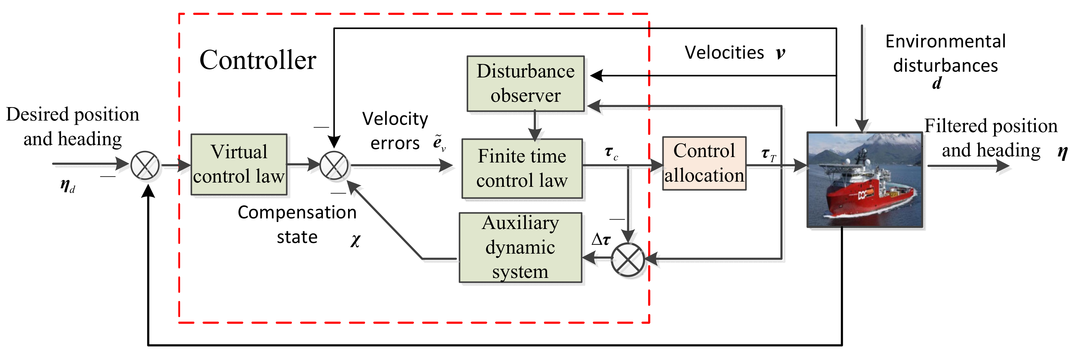In other studies, such as [19,20,21,22,23,24,25], the physical properties of the thruster are not fully considered. Therefore, focusing on unknown time-varying disturbances and actuator constraints in this paper. We present a disturbance observer-based finite-time control scheme with control allocation for DP systems for ships. The finite-time disturbance observer is used to estimate the unknown time-varying disturbances, the control allocation is applied online to inform the controller about actuator saturation, and the auxiliary system dynamic is constructed to handle velocity deviation. Furthermore, the closed-loop system has finite-time stability. To the best of the authors’ knowledge, this is the first published study of DP control design that both considers finite-time disturbance suppression and presents an auxiliary dynamic system designed for a joint system. The main contributions of this paper are as follows:

(i)

An adaptive finite-time disturbance observer is constructed to estimate unknown time-varying disturbances. It does not require prior information about the disturbances and can eliminate undesired chattering.

(ii)

An auxiliary dynamic system is constructed to handle the input constraints. It reduces the tracking deviation caused by the mismatch between the forces produced by the thruster system and the desired control law.

(iii)

By combining control design and control allocation, a finite-time control scheme with a disturbance observer and an auxiliary dynamic system is presented; this scheme can achieve disturbance suppression and handle actuator constraints. Due to the fast exponential reaching law, the controller reduces undesired chattering.

The paper is organized as follows. Preliminaries and problem formulations are described in Section 2. The two finite-time disturbance observers, the control design, and the control allocation are given in Section 3; in this section, we also propose the finite-time controller with a disturbance observer and an auxiliary dynamic system for ship DP systems. The results and discussion are presented in Section 4. Conclusions are drawn in Section 5.

2. Problem Formulation and Preliminaries

2.1. DP Ship Dynamics

The three degree of freedom DP system for ships is only concerned with low-frequency horizontal motions where two coordinate systems are defined, as shown in Figure 1. We denote the position vector $\eta ={[x,y,\psi ]}^T$ in the Earth-fixed frame O_EX_EY_E, and the velocity vector $v={[u,v,r]}^T$ in the body-fixed frame OXY. Here, the relative direction of the wind, the currents, and the waves (${\theta }_{\mathrm{w}}$, ${\theta }_c$, and ${\theta }_{\mathrm{wa}}$) are defined according to O_EX_E:

The damping force can be approximated as linear at low speed, so the DP’s dynamic model of ships with environmental disturbances is expressed as:

$$\{\begin{array}{l}\dot{\eta }=J(\psi )v\\ M\dot{v}+Dv={\tau }_T+{\tau }_{wind}+{\tau }_{wave}+{\tau }_{cu}\end{array}$$

(1)

where the rotation matrix $J(\psi )$ is:

$$J(\psi )=\left[\begin{array}{ccc}\cos \psi & -\sin \psi & 0\\ \sin \psi & \cos \psi & 0\\ 0& 0& 1\end{array}\right]$$

$M\in R^{3\times 3}$ denotes the invertible and positive definite inertia matrix. $D\in R^{3\times 3}$ is the damping matrix. ${\tau }_T=[{\tau }_{T1},{\tau }_{T2},{\tau }_{T3}{]}^T$ is the thruster system’s actual control vector.

The compound environmental disturbance vector is defined as $d(t)={[d_1(t),d_2(t),d_3(t)]}^T$; that is:

$$d(t)={\tau }_{wind}+{\tau }_{wave}+{\tau }_{cu}$$

(2)

where ${\tau }_{wind}\in R^3$ is the wind force and moment, ${\tau }_{wave}\in R^3$ is the second-order wave force and moment, and ${\tau }_{cu}\in R^3$ is the current force and moment.

Let ${\tau }_c={[{\tau }_{c1},{\tau }_{c2},{\tau }_{c3}]}^T$ be the command control law consisting of forces and moment, as calculated by the DP controller.

Remark 1.

Sea states are constantly changing and have limited energy, so environmental disturbances that act on the ship are time-varying and bounded. Additionally, the upper bound of the disturbances can be roughly calculated using the wind and current load coefficients obtained from the wind tunnel test and the second-order wave force transfer functions obtained by numeral calculations. Therefore, we arrive at the following assumption:

Assumption 1.

The environmental disturbance terms $d_i(t),i=1,2,3$ are unknown, bounded, and time-varying. The upper bound of the disturbances$l_i, i=1,2,3$can be roughly calculated and satisfy$|d_i(t)|{\le }_{ }{l}_i$.

2.2. Preliminaries

In this subsection, some lemmas are recalled that will be used in the control design.

For two same-size vectors $\mathit{x}={[x_1,\cdots ,x_n]}^T$ and $\mathit{y}={[y_1,\cdots ,y_n]}^T$, the Hadamard product of $\mathit{x}$ and $\mathit{y}$ is defined as $\mathit{x}\circ \mathit{y}={[x_1{y}_1,\cdots ,x_n{y}_n]}^T$. For $0<r<1$, $\mathrm{sgn}(\cdot )$ is the signum function, denoting that $\mathrm{sgn}(\mathit{x})={[\mathrm{sgn}(x_1),\cdots ,\mathrm{sgn}(x_n)]}^T$ and ${\mathrm{sgn}}^r(x)={[|x_1{|}^r\mathrm{sgn}(x_1),\cdots ,|x_n{|}^r\mathrm{sgn}(x_n)]}^T$.

The notation $||\cdot ||$ refers to the Euclidean norm of a vector. ${\lambda }_{\max }(\cdot )$ and ${\lambda }_{\min }(\cdot )$ denote the maximum and minimum eigenvalues of a matrix, respectively.

Lemma 1.

(Hardy et al. [28]) For$x_i\in R,i=1,\cdots ,n$and $0<q<1$, the following inequality is satisfied:

$$|x_1{|}^{1+q}+\cdots +|x_n{|}^{1+q}\ge {(|x_1{|}^2+\cdots +|x_n{|}^2)}^{(1+q)/2}$$

(3)

Lemma 2.

(Yu et al. [29]) For a system$\dot{x}=f(x,t)$: if there exist ${\lambda }_1>0$,${\lambda }_2>0$ and $0<a<1$, the continuous function$V(x)$(defined on $U\subset R^n$) satisfies the following inequality:

$$\begin{array}{l}\dot{V}(x)+{\lambda }_2{V}^a(x)\le 0,\\ \dot{V}(x)+{\lambda }_{1}V(x)+{\lambda }_2{V}^a(x)\le 0\end{array}$$

(4)

Then, $V(x)$ with the initial value $V(x_0)$ can reach $V(x)\equiv 0$ in finite time, and the trajectory of the system is finite-time stable. The setting time is bounded as:

$$\begin{array}{l}T\le \frac{1}{{\lambda }_2(1-a)}{V}^{1-a}(x_0)\\ T\le \frac{1}{{\lambda }_1(1-a)}\ln \frac{{\lambda }_1{V}^{1-a}(x_0)+{\lambda }_2}{{\lambda }_2}\end{array}$$

(5)

Lemma 3.

(Zhu et al. [30]) For a system$\dot{x}=f(x,t)$, the solution is finite-time stable if$x(t)=0$ is constantly established for all $t>T(x_0)$. Then, if there exist $\epsilon >0$ and $T(\epsilon ,x_0)<\infty$ with $x(t_0)=x_0$, such that $||x(t)||<\epsilon$, for all $t>T(\epsilon ,x_0)+t_0$, the solution is practical finite-time stable (PFS). Suppose that there exists a positive definite function $V(x)$, for ${\lambda }_1>0$, $0<a<1$, and $0<\eta <\infty$, such that $\dot{V}(x)+{\lambda }_2{V}^a(x)\le \eta$. The solution trajectory is PFS. The setting time is bounded as:

$$T\le \frac{1}{\theta {\lambda }_2(1-a)}{V}^{1-a}(x_0)$$

(6)

where $0<\theta <1$.

2.3. Control Objective

Taking into account the DP system given by (1), with unknown time-varying disturbances and actuator constraints, under Assumption 1, a finite-time control law ${\tau }_c$ is designed such that the DP system for ships can track the predetermined trajectories ${\eta }_d={[x_d,y_d,{\psi }_d]}^T$.

The benefits of the designed controller are as follows: (1) it achieves disturbance suppression in finite time without any prior knowledge of the disturbances; (2) the controller receives information online about actuator saturation and compensates for the tracking errors caused by the actuator constraints; (3) it guarantees that the position and heading tracking errors converge to zero in finite time; (4) it reduces undesired chattering.

3. Finite-Time Control Design

In this section, a finite-time DP control law is developed by combining the control design and the control allocation algorithm with the aid of TSM. Two finite-time disturbance observers are designed to estimate the unknown time-varying yet bounded disturbances, and the auxiliary dynamic system is proposed to compensate for errors caused by the mismatch of forces produced by the thruster system and the DP control law.

3.1. Disturbance Observer Design

3.1.1. SMDO Design

In this subsection, to estimate the disturbances $d(t)$, a sliding-mode disturbance observer (SMDO) is designed. First, an auxiliary sliding variable is selected as:

$$\begin{array}{l}{s}_{do}=\xi -v\\ M\dot{\xi }=-L_d\circ \mathrm{sgn}(s_{do})-{\epsilon }_0{\mathrm{sgn}}^r(s_{do})+{\tau }_T-Dv\end{array}$$

(7)

where $s_{do}\in R^3$, $\xi \in R^3$ are vectors of the sliding surface and the auxiliary variable, respectively; the design matrix ${\epsilon }_0\in R^{3\times 3}$ is a positive definite diagonal, $0<r<1$; and $L_d={[l_1,l_2,l_3]}^T$ is defined by the upper bound of environmental disturbances.

The estimated vector $\widehat{d}(t)$ is proposed to be:

$$\widehat{d}(t)=-L_d\circ \mathrm{sgn}(s_{do})-{\epsilon }_0{\mathrm{sgn}}^r(s_{do})$$

(8)

Because of (1), (7), and (8), we obtain:

$$\begin{array}{l}M{\dot{s}}_{do} =-L_d\circ \mathrm{sgn}(s_{do})-{\epsilon }_0{\mathrm{sgn}}^r(s_{do})+{\tau }_T-Dv-(-Dv+{\tau }_T+d) \\ =-L_d\circ \mathrm{sgn}(s_{do})-{\epsilon }_0{\mathrm{sgn}}^r(s_{do})-d=\tilde{d}\end{array}$$

(9)

where $\tilde{\mathit{d}}=\widehat{d}-d$ is the disturbance estimate error vector. From (9), we can conclude that, if the auxiliary sliding variable dynamic ${\dot{s}}_{do}\to 0$, then $\tilde{\mathit{d}}\to 0$.

The Lyapunov function candidate is selected as:

$$V_{do}=\frac{1}{2}{s}_{do}^{T}M{s}_{do}$$

(10)

Using (7), (8), and (9), the derivative of (10) is:

$${\dot{V}}_{do}=s_{do}^{T}M{\dot{s}}_{do} =s_{do}^T[-L_d\circ \mathrm{sgn}(s_{do})-{\epsilon }_0{\mathrm{sgn}}^r(s_{do})-d ]$$

(11)

Note that, in Assumption 1, the environmental disturbances are bounded. It is known that the upper bound $L_d$ can be roughly obtained through experiments and calculations. Thus, the following inequalities hold:

$$\begin{array}{l}-s_{do}^{T}d\le |s_{do}^{T}d| \le |s_{do}^T|L_d\Rightarrow -|s_{do}^T|L_d-s_{do}^{T}d\le 0\\ \iff -s_{do}^T[L_d\circ \mathrm{sgn}(s_{do})]-s_{do}^{T}d\le 0 \end{array}$$

(12)

Using (12), and according to Lemma 1, we obtain the following:

$${\dot{V}}_{do} \le -{\lambda }_{\min }({\epsilon }_0){(||s_{do}|{|}^2)}^{\frac{1+r}{2}}$$

(13)

From (10), ${\lambda }_{\min }(M)s_{do}^T{s}_{do}\le s_{do}^{T}M{s}_{do}\le {\lambda }_{\max }(M)s_{do}^T{s}_{do}$ holds, so we obtain:

$${\dot{V}}_{do} \le -\kappa V_{do}^{\frac{1+r}{2}}$$

(14)

where $\kappa =\frac{{\lambda }_{\min }({\epsilon }_0)}{{[{\lambda }_{\max }(M)/2]}^{(1+r)/2}}$.

Clearly, $\frac{1}{2}<\frac{1+r}{2}<1$, according to Lemma 2; thus, it can be determined that the decrease in the Lyapunov function $V_{do}$ can drive the trajectories of the SMDO onto the sliding surface $s_{do}=0$ in finite time, which implies that $\widehat{d}$ can effectively estimate the bounded disturbances $d$ in finite time. Furthermore, the parameter $\kappa$ to be designed determines the setting time. It can be shown that the setting time satisfies:

$$T_{do}\le \frac{1}{\kappa (1-\frac{1+r}{2})}{V}_{do}^{1-\frac{1+r}{2}}(0)$$

(15)

We note that $s_{do}\to 0$ and is then to be kept zero, which leads to ${\dot{s}}_{do}\to 0$. Thus, from (9), the disturbance estimate error vector $\tilde{\mathit{d}}\to 0$ holds, and the convergence rate can be made as fast as possible by selecting the appropriate parameter ${\epsilon }_0$. Therefore, the following theorem holds:

Theorem 1.

Considering the DP system given by (1) with Assumption 1, the disturbance estimation error vector$\tilde{\mathit{d}}(t)$of the SMDO constructed by (7) and (8) can converge to zero in finite time, as quickly as possible, by selecting the appropriate parameter${\epsilon }_0$.

3.1.2. ADO Design

We know that the disturbances $d(t)$ can be effectively estimated in finite time using (7) and (8). However, the upper bound of the disturbances can only be calculated roughly. Moreover, the high-frequency switching value $\widehat{d}(t)$ given by (8) may degrade the performance of the DP control system. Therefore, in order to modify the SMDO, an adaptive scheme is proposed to estimate the upper bound of disturbances $l_i,i=1,2,3$. As such, we obtain the adaptive disturbance observer (ADO).

The adaptation update law is defined as:

$${\dot{\widehat{L}}}_d=-K_0{\widehat{L}}_d+M|s_{do}|$$

(16)

where $K_0=\mathrm{diag}(k_{01},k_{02},k_{03})$ is a positive definite design matrix, ${\widehat{L}}_d={[{\widehat{l}}_1,{\widehat{l}}_2,{\widehat{l}}_3]}^T$ is a vector defined by the estimates of the upper bound of the disturbances, and $|s_{do}|={[|s_{do1}|,|s_{do2}|,|s_{do3}|]}^T$. Therefore, the designed ADO is, practically, finite-time stable.

Considering the Lyapunov function candidate as:

$${\overline{V}}_{do}=\frac{1}{2}{s}_{do}^{T}M{s}_{do}+ \frac{1}{2}{\tilde{\mathit{L}}}_d^T{M}^{-1}{\tilde{\mathit{L}}}_d$$

(17)

where ${\tilde{\mathit{L}}}_d=L_d-{\widehat{L}}_d$, its time derivative is:

$$\begin{array}{l}{\dot{\overline{V}}}_{do}=s_{do}^{T}M{\dot{s}}_{do}- {\tilde{L}}_d^T{M}^{-1}{\dot{\widehat{L}}}_d\\ =-s_{do}^T[{\widehat{L}}_d\circ \mathrm{sgn}(s_{do})]-s_{do}^T{\epsilon }_0{\mathrm{sgn}}^r(s_{do})-s^{T}d +{\tilde{L}}_d^T{K}_0{\widehat{L}}_d-{\tilde{L}}_d^T|s_{do}|\end{array}$$

(18)

As has been established, the following inequality holds:

$${\tilde{\mathit{L}}}_d^T{K}_0{\widehat{L}}_d=-{\tilde{\mathit{L}}}_d^T{K}_0{\tilde{\mathit{L}}}_d+{\tilde{\mathit{L}}}_d^T{K}_0{L}_d\le -[{\lambda }_{\min }(K_0)-\frac{1}{2}]{\tilde{\mathit{L}}}_d^T{\tilde{\mathit{L}}}_d+{\displaystyle \sum _{i=1}^3\frac{K_{0i}^2{L}_{di}^2}{2}}$$

(19)

Using (12) and (19), Equation (18) can be expressed as:

$$\begin{array}{ll}{\dot{\overline{V}}}_{do}& \le -s_{do}^T{\epsilon }_0{\mathrm{sgn}}^r(s_{do}) +{\tilde{L}}_d^T{K}_0{\widehat{L}}_d\\ & \le -{\lambda }_{\min }({\epsilon }_0){(||s_{do}|{|}^2)}^{\frac{1+r}{2}}-[{\lambda }_{\min }(K_0)-\frac{1}{2}]{\tilde{L}}_d^T{\tilde{L}}_d +{\displaystyle \sum _{i=1}^3\frac{k_{0i}^2{L}_{di}^2}{2}}\\ & \le -\kappa {(\frac{1}{2}{s}_{do}^{T}M{s}_{do})}^{\frac{1+r}{2}}-[{\lambda }_{\min }(K_0)-\frac{1}{2}]{({\tilde{L}}_d^T{\tilde{L}}_d)}^{\frac{1+r}{2}}+[{\lambda }_{\min }(K_0)-\frac{1}{2}][{({\tilde{L}}_d^T{\tilde{L}}_d)}^{\frac{1+r}{2}}-{\tilde{L}}_d^T{\tilde{L}}_d]+{\displaystyle \sum _{i=1}^3\frac{k_{0i}^2{L}_{di}^2}{2}}\end{array}$$

(20)

where ${\lambda }_{\min }(K_0)>\frac{1}{2}$. Furthermore, consider the following two cases:

(i)

When $||{\tilde{\mathit{L}}}_d|| >1$, ${({\tilde{L}}_d^T{\tilde{L}}_d)}^{\frac{1+r}{2}}-{\tilde{\mathit{L}}}_d^T{\tilde{\mathit{L}}}_d<0$, we have:

$${\dot{\overline{V}}}_{do}\le -\kappa {(\frac{1}{2}{s}_{do}^{T}M{s}_{do})}^{\frac{1+r}{2}}-[{\lambda }_{\min }(K_0)-\frac{1}{2}]{({\tilde{L}}_d^T{\tilde{L}}_d)}^{\frac{1+r}{2}} +{\displaystyle \sum _{i=1}^3\frac{k_{0i}^2{L}_{di}^2}{2}}$$

(21)

(ii)

When $||{\tilde{\mathit{L}}}_d|| \le 1$, we have:

$$[{\lambda }_{\min }(K_0)-\frac{1}{2}]{({\tilde{L}}_d^T{\tilde{L}}_d)}^{\frac{1+r}{2}}{|}_{||{\tilde{L}}_d|| \le 1}<[{\lambda }_{\min }(K_0)-\frac{1}{2}]{({\tilde{L}}_d^T{\tilde{L}}_d)}^{\frac{1+r}{2}}{|}_{||{\tilde{L}}_d|| >1}$$

(22)

Therefore, from (21) and (22), according to Lemma 1, we obtain:

$$\begin{array}{ll}{\dot{\overline{V}}}_{do}& \le -\kappa {(\frac{1}{2}{s}_{do}^{T}M{s}_{do})}^{\frac{1+r}{2}}-[{\lambda }_{\min }(K_0)-\frac{1}{2}]{({\tilde{L}}_d^T{\tilde{L}}_d)}^{\frac{1+r}{2}} +{\displaystyle \sum _{i=1}^3\frac{k_{0i}^2{L}_{di}^2}{2}}\\ & \le -\overline{\kappa }{\overline{V}}_{do}{}^{\frac{1+r}{2}} +\overline{\eta }\end{array}$$

(23)

where $\overline{\kappa }=\min \{\kappa ,\frac{{\lambda }_{\min }(K_0)-1/2}{{(1/2)}^{(1+r)/2}}\}$ and $\overline{\eta }={\displaystyle \sum _{i=1}^3\frac{k_{0i}^2{L}_{di}^2}{2}}$. According to Lemma 3, the decrease in ${\overline{V}}_{do}$ can drive the trajectories of the SMDO into ${\overline{V}}_{do}{}^{\frac{1+r}{2}} \le \overline{\eta }/[(1-\theta )\overline{\kappa }],0<\theta <1$ in finite time, and the trajectories of the SMDO are bounded as:

$$\underset{t\to T}{\lim }{s}_{do}(t)\in (||s_{do}||\le \sqrt{\frac{2}{{\lambda }_{\min }(M)}}{(\frac{\overline{\eta }}{(1-\theta )\overline{\kappa }})}^{\frac{2}{1+r}})$$

(24)

Furthermore, in light of (17), we know that ${\tilde{\mathit{L}}}_d$ is bounded. Furthermore, we can see from (7)–(9) that ${\dot{\mathit{s}}}_{do}$ and $\tilde{\mathit{d}}$ are bounded.

3.2. Finite-Time Control Design

In this section, a finite-time control law is developed for the ship DP system; this law is combined with the designed system, the disturbance observer, and the auxiliary dynamic system. The structure of the DP system is shown in Figure 2.

Based on the backstepping technique, the design process is given as follows:

Step 1:

Define the position error vector $e_{\eta }={[e_x,e_y,e_{\psi }]}^T$ as:

$$e_{\eta }=\eta -{\eta }_d$$

(25)

Its time derivative is:

$${\dot{e}}_{\eta }=J(\psi )v-{\dot{\eta }}_{\mathrm{d}}$$

(26)

Let $v$ be a virtual control input, and design an intermediate control vector $\varphi$ as:

$$\varphi =J^T(\psi )[-K_1 e_{\eta }-{\epsilon }_1{\mathrm{sgn}}^r(e_{\eta })+{\dot{\eta }}_{\mathrm{d}}]$$

(27)

where $K_1=K_1^T\in R^{3\times 3}$ and ${\epsilon }_1={\epsilon }_1^T\in R^{3\times 3}$ are positive definite design matrices, and $0<r<1$.

Define the velocity error vector $e_v={[e_u,e_v,e_r]}^T$ as $e_v=v-\varphi$. Then, (26) can be written as:

$${\dot{\mathit{e}}}_{\eta }=-K_1 e_{\eta }-{\epsilon }_1{\mathrm{sgn}}^r(e_{\eta })+J(\psi )e_v$$

(28)

Step 2:

Here, for the second subsystem of (1), the control law ${\tau }_c$ will be defined to make $v$ track its command $\varphi$ even when the actuator constraints are in effect. Note that, considering the actuator constraints, there may be deviations between the defined control law ${\tau }_c$ and the forces ${\tau }_T$ produced by the thrusters, which will result in an increase in velocity tracking errors. In order to compensate for these errors, an auxiliary dynamic system is constructed as follows:

$$\dot{\mathit{\chi }}=-K_{\chi }\arctan \chi +M^{-1}({\tau }_T-{\tau }_c)$$

(29)

where $\chi ={[{\chi }_1,{\chi }_2,{\chi }_3]}^T$ is the state vector, and the design matrix $K_{\chi }\in R^{3\times 3}$ is positive definite.

Define the compensated tracking error vector as:

$${\tilde{e}}_v=e_v-\chi$$

(30)

From (1) and (29), the time derivative of ${\tilde{\mathit{e}}}_v$ is:

$${\dot{\tilde{\mathit{e}}}}_v=\dot{v}-\dot{\varphi }-\dot{\chi } =M^{-1}[-Dv+d]-\dot{\varphi }+K_{\chi }\arctan \chi +M^{-1}{\tau }_c$$

(31)

Then, for finite-time convergence of the DP control system, a TSM surface $s_v={[s_{v1},s_{v2},s_{v3}]}^T$ is chosen as:

$$s_v={\tilde{\mathit{e}}}_v+\lambda {\displaystyle {\int }_0^t{\mathrm{sgn}}^{\rho }({\tilde{\mathit{e}}}_v)}+s_{do}$$

(32)

where $\lambda =\mathrm{diag}({\lambda }_1,{\lambda }_2,{\lambda }_3)$ is a positive definite design matrix, and the design constant $0<\rho <1$.

Define a fast exponential reaching law:

$${\dot{\mathit{s}}}_v=-K_2{s}_v-{\epsilon }_2{\mathrm{sgn}}^r(s_v)$$

(33)

where $K_2=K_2^T\in R^{3\times 3}$ and ${\epsilon }_2={\epsilon }_2^T\in R^{3\times 3}$ are positive definite design matrices.

The finite-time control law, consisting of the disturbance observer and the auxiliary dynamic system, is as follows:

$$\begin{array}{l}{\tau }_c={\tau }_0+{\tau }_1\\ {\tau }_0=-M{K}_2{s}_v-M{\epsilon }_2{\mathrm{sgn}}^r(s_v)\\ {\tau }_1=Dv-\widehat{d}+M[\dot{\varphi }-\lambda {\mathrm{sgn}}^{\rho }({\tilde{\mathit{e}}}_v)-K_{\chi }\arctan \chi ]-\Theta e_{\eta }^{T}J(\psi )e_v\end{array}$$

(34)

where $\Theta ={[1/s_{v1},1/s_{v2},1/s_{v3}]}^T/3$.

From (31), and substituting (34) into the time derivative of $s_v$, we have:

$$\begin{array}{ll}M{\dot{\mathit{s}}}_v& =-Dv+d- M\dot{\varphi }+M{K}_{\chi }\arctan \chi +{\tau }_c+M\lambda {\mathrm{sgn}}^{\rho }({\tilde{\mathit{e}}}_v)+M{\dot{\mathit{s}}}_{do}\\ & =-M{K}_2{s}_v-M{\epsilon }_2{\mathrm{sgn}}^r(s_v)-(\widehat{d}-d)+M{\dot{\mathit{s}}}_{do}-\Theta e_{\eta }^{T}J(\psi )e_v\end{array}$$

(35)

We note that, in (9), ${\dot{\mathit{s}}}_{do} =\mathit{M}\tilde{\mathit{d}}$, and then we have:

$$M{\dot{\mathit{s}}}_v=-M{K}_2{s}_v-M{\epsilon }_2{\mathrm{sgn}}^r(s_v)-\Theta e_{\eta }^{T}J(\psi )e_v$$

(36)

Theorem 2.

For the ship DP system (1) with Assumption 1: choose the appropriate design matrices $K_0$, $K_1$, $K_2$, ${\epsilon }_0$, ${\epsilon }_1$, ${\epsilon }_2$, and $K_{\chi }$, and the design constants $\lambda$, $\rho$ and $r$, such that the designed controller can guarantee $e_{\eta }\to 0$, $s_v\to 0$, and the boundedness of other signals in finite time, where the controller includes the virtual law (27); actual control law (34); the ADO given by (7), (8), and (16); and the auxiliary dynamic system given by (29).

Proof of Theorem 2.

From (35) and (36), it is determined that the time derivative of $s_v$ is not affected by the bounded ADO. Furthermore, to better simplify the parameter design, we try our best to choose the Lyapunov function based on the original dynamic model. Therefore, according to the form of Equation (36), the Lyapunov function is selected as:

$$V=\frac{1}{2}{e}_{\eta }^T{e}_{\eta }+\frac{1}{2}{s}_v^{T}M{s}_v$$

(37)

According to (29) and (36), the time derivative of (37) yields:

$$\begin{array}{ll}\dot{V}& =e_{\eta }^T[-K_1 e_{\eta }-{\epsilon }_1{\mathrm{sgn}}^r(e_{\eta })]+s_v^T[-M{K}_2{s}_v-M{\epsilon }_2{\mathrm{sgn}}^r(s_v)]\\ & \le -{\lambda }_{\min }(K_1)||e_{\eta }|{|}^2-{\lambda }_{\min }(K_2)s_v^{T}M{s}_v -{\lambda }_{\min }({\epsilon }_1){(|e_{\eta }|{ }^2)}^{\frac{1+r}{2}}-{\lambda }_{\min }(M{\epsilon }_2){(|s_v|{ }^2)}^{\frac{1+r}{2}}\\ & \le -KV -\varpi V\end{array}$$

(38)

where $K=\min \{2{\lambda }_{\min }(K_1),2{\lambda }_{\min }(K_2)\}$ and $\varpi =\min \{2^{\frac{1+r}{2}}{\lambda }_{\min }({\epsilon }_1),\frac{{\lambda }_{\min }(M{\epsilon }_2)}{{[{\lambda }_{\max }(M)/2]}^{(1+r)/2}}\}$.

According to Lemma 2, the decrease in the Lyapunov function $V$ can drive the sliding surface vector $s_v\to 0$ and the tracking error vector $e_{\eta }\to 0$ in finite time. The setting time is:

$$T_V=\frac{1}{K(1-\frac{1+r}{2})}\ln \frac{K{V}^{1-\frac{1+r}{2}}(0)+\varpi }{\varpi }$$

(39)

Therefore, the DP ship can track the desired trajectories ${\eta }_d={[x_d,y_d,{\psi }_d]}^T$ in finite time under the designed control law.

Now, we have obtained $s_v\to 0$. Furthermore, in light of (32), the compensated velocity errors ${\tilde{\mathit{e}}}_v$ reach the sliding surface and stay on it forever; we integrate both sides of Equation (32) and we have ${\dot{\tilde{\mathit{e}}}}_v+\lambda |{\tilde{\mathit{e}}}_v{|}^{\rho }+{\dot{\mathit{s}}}_{do}=0$. Moreover, taking into account the results of Lemma 3 and Theorem 1, we can deduce that the compensated tracking errors ${\tilde{\mathit{e}}}_v$ are bounded, and the band of the bounded region is determined by the range of ${\dot{\mathit{s}}}_{do}$. This concludes the proof. □

Remark 2.

The compensation application technique has been used in the input constraint control systems in [14,15,16,17]. However, this present study represents the first time in the literature where both the auxiliary dynamic system has been employed to compensate for errors induced by the mismatch between${\tau }_T$and${\tau }_c$in DP control design, and that the state vector$\chi$is bounded.

To prove that the state vector $\chi$ is bounded, consider another Lyapunov function candidate as $V_{\chi }=\frac{1}{2}{\chi }^T\chi$, whereby the derivative of $V_{\chi }$ is:

$${\dot{V}}_{\chi }={\chi }^T[-K_{\chi }\arctan \chi +M^{-1}({\tau }_T-{\tau }_c)]$$

(40)

Let $|{\tau }_T-{\tau }_c|\le {\tau }_M$. Here, ${\tau }_M$ is a positive constant vector. Then, (40) can be written as:

$${\dot{V}}_{\chi }\le -{\lambda }_{\min }(K_{\chi }){\chi }^T\arctan \chi +|{\chi }^T|M^{-1}{\tau }_M$$

(41)

By the selections of $K_{\chi }$, we can make ${\lambda }_{\min }(K_{\chi })>\frac{M^{-1}{\tau }_M}{|\arctan \chi |}$, then ${\dot{V}}_{\chi }<0$. Therefore, $\chi$ is bounded. Clearly, $e_v$ is bounded due to ${\tilde{\mathit{e}}}_v=e_v-\chi$. Furthermore, if ${\tau }_T={\tau }_c$, we can determine that $\chi =0$ is a particular solution of (29); then, ${\tilde{e}}_v=e_v$, and $e_v$ is still bounded.

Remark 3.

The constant $r$ in (7), (27), and (33) can be different, depending on the performance of the DP control system. According to Theorems 1 and 2, we can see that the design parameter$0<r<1$is related to the convergence rate of the system directly from (15) and (39). Taking as an example the finite-time control, it can be seen from the given reaching law (33) that the approach rate is mainly determined by the exponential term when the sliding surface vector $s_v$ is small. Therefore, the parameter $r$ is usually chosen to be small enough to speed up the convergence of the system; however, if $r$ is too small, it will increase the control input chattering and easily cause system instability.

3.3. Control Allocation

The control allocation is used to find the optimal thruster forces and direction corresponding to the controller, which can be taken as an optimization problem with cost functions and constraints. The previously presented methods for control allocation can be found in [19,31]. The unconstrained nonlinear optimization problems are formulated using Lagrange multipliers in [31,32]. However, this solution is not optimal when considering time-varying thrust directions. In this paper, the control allocation problems can be solved as nonlinearly constrained problems by considering physical limitations to the thrusters that restrict the set of admissible thrusts and azimuth angles [31,33,34].

The cost functions are formulated as follows [34]:

$$\mathrm{J}(\alpha ,f,s)=f^{T}Qf+{(\alpha -{\alpha }_0)}^{T}U(\alpha -{\alpha }_0)+s^{T}Ws$$

(42)

where $\mathrm{J}$ is a cost function, $f$ is a thrust vector, $f_0$ and ${\alpha }_0$ are, respectively, the thrust and azimuth angle at the previous sample time, $\alpha \in R^n$ is the azimuth angle vector at the current sample time, and $s\in R^3$ is a vector of slack variables, which is introduced to ensure the existence of a solution. $Q\in R^{n\times n}$ and $U\in R^{n\times n}$ are weighting matrices, and the matrix $W\in R^{3\times 3}$ is significantly larger to force the optimal solution $s\approx 0$.

The equality constraint ensures that the controlled forces and moments are produced. It should be taken into consideration that there are physical limitations on the thrust and turning rate of the azimuth angle, which can be expressed as follows [34,35]:

$$s+B\left(\alpha \right)f={\tau }_c$$

(43)

$$\begin{array}{l}{f}_{\min }\le f\le f_{\max },\Delta f_{\min }\le f-f_0\le \Delta f_{\max }\\ {\alpha }_{\min }\le \alpha \le {\alpha }_{\max },\Delta {\alpha }_{\min }\le \alpha -{\alpha }_0\le \Delta {\alpha }_{\max }\end{array}$$

(44)

where $B\left(\alpha \right)$ denotes the thruster configuration matrix, $f_{\max }\in R^n$ denotes the maximum thrust vector, $f_{\min }\in R^n$ denotes the minimum thrust vector, maximum $\Delta f_{\max }\in R^n$ and minimum $\Delta f_{\min }\in R^n$ are turning rates of the thrusters, and maximum $\Delta {\alpha }_{\max }\in R^n$ and minimum $\Delta {\alpha }_{\min }\in R^n$ are rates of change of azimuth angles. The optimization problem described above can be solved by sequential quadratic programming (SQP) [36,37].

In the following simulation, the control allocation algorithm (42)–(44) is applied.

4. Results and Discussions

To evaluate the effectiveness of the control scheme proposed in Section 3, we present simulations of a cable-laying ship with a DP system. The main information about the ship is listed in

Table 1. Overview of the ship.

Parameter	Symbol	Unit	Ship
Overall length	L	m	57.6
Breadth	B	m	22.0
Depth	D	m	4
Design draft	T	m	2.3
Displacement	Δ	ton	1527.4

.

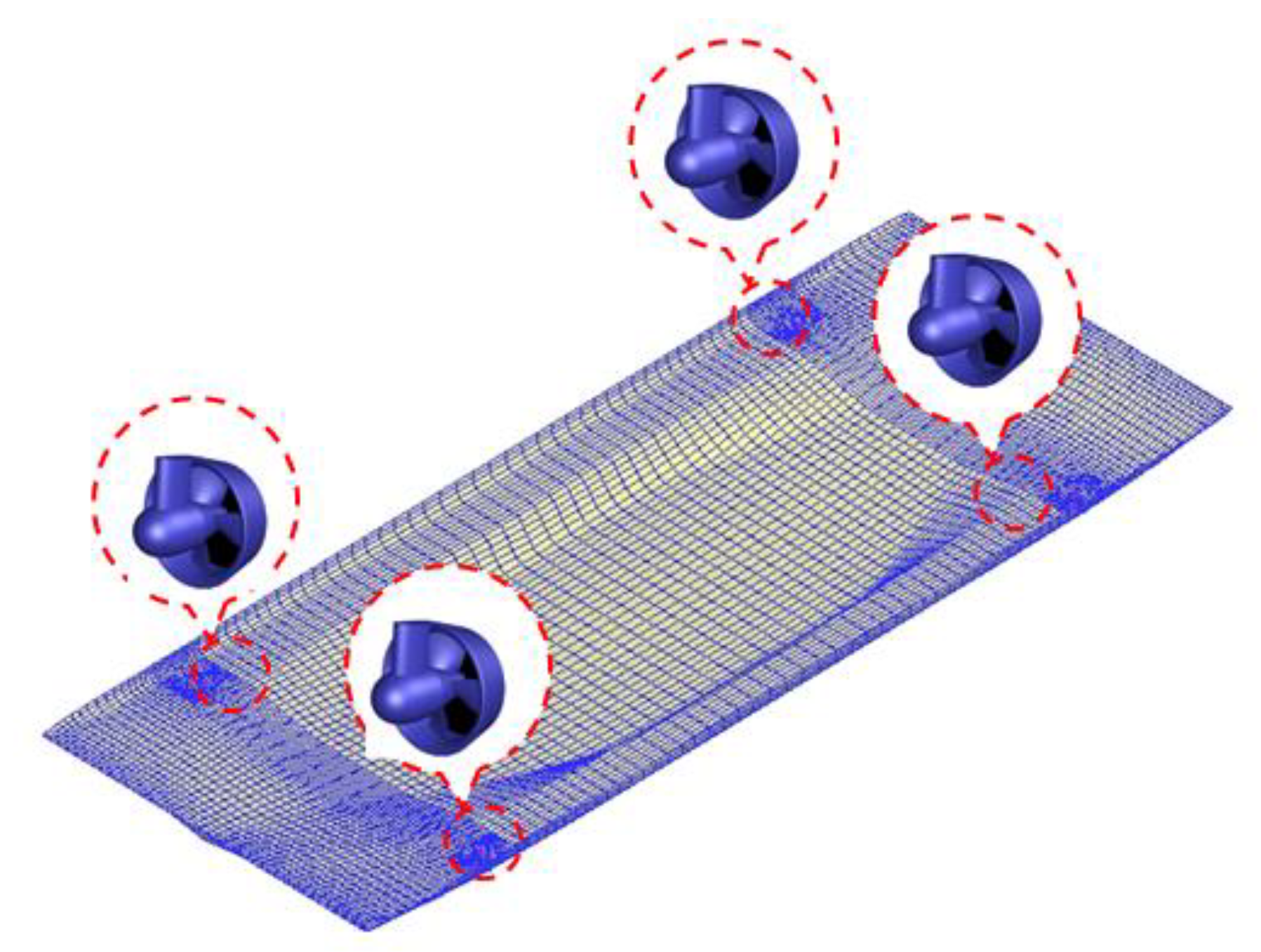
The ship is equipped with four same-type azimuth thrusters (two located aft and two in the fore). The four azimuth thrusters are fixed-pitch, with a maximum thrust of 65 kN in open water, and are symmetric along the longitudinal and transverse middle sections. The sketch of thruster positions is shown in Figure 3.

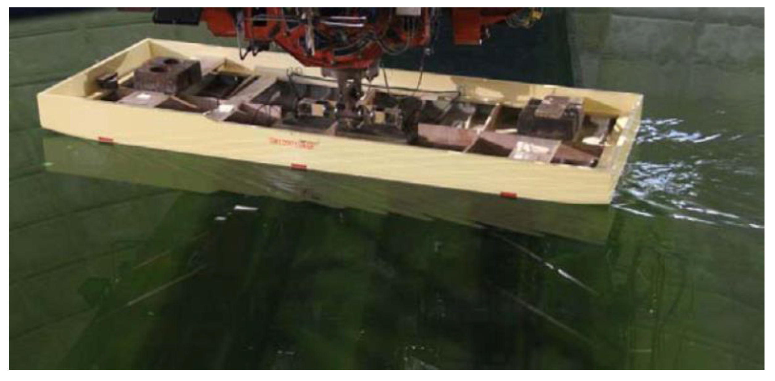
In order to obtain the inertia matrix $M$ and the damping matrix $D$, a 1/25 captive model test was carried out at the China Ship Scientific Research Center (CSSRC). The test photo is shown in Figure 4.

Additionally, the parameters of the ship’s dynamic model are given as follows:

$$M=\left|\begin{array}{ccc}1.610242\times {10}^6\hfill & 0& \hfill 0\\ 0\hfill & 2.18685\times {10}^6& \hfill 0\\ 0\hfill & 0& \hfill 4.2522\times {10}^8\end{array}\right|, D=\left|\begin{array}{ccc}6.59397\times {10}^2\hfill & 0& \hfill 0\\ 0\hfill & 1.018375\times {10}^3& \hfill 3.501\times {10}^4\\ 0\hfill & 2.187\times {10}^4& \hfill 3.3566\times {10}^5\end{array}\right|$$

The marine environmental parameters are given in

Table 2. Marine environmental parameters.

Case No.	Wave		Wind Speed/kn	Current Speed/kn
	Significant Wave Height H1/3/m	Periods T01/s
1	1.5	6.0	7	2
2	2.5	7.0	15	2

.

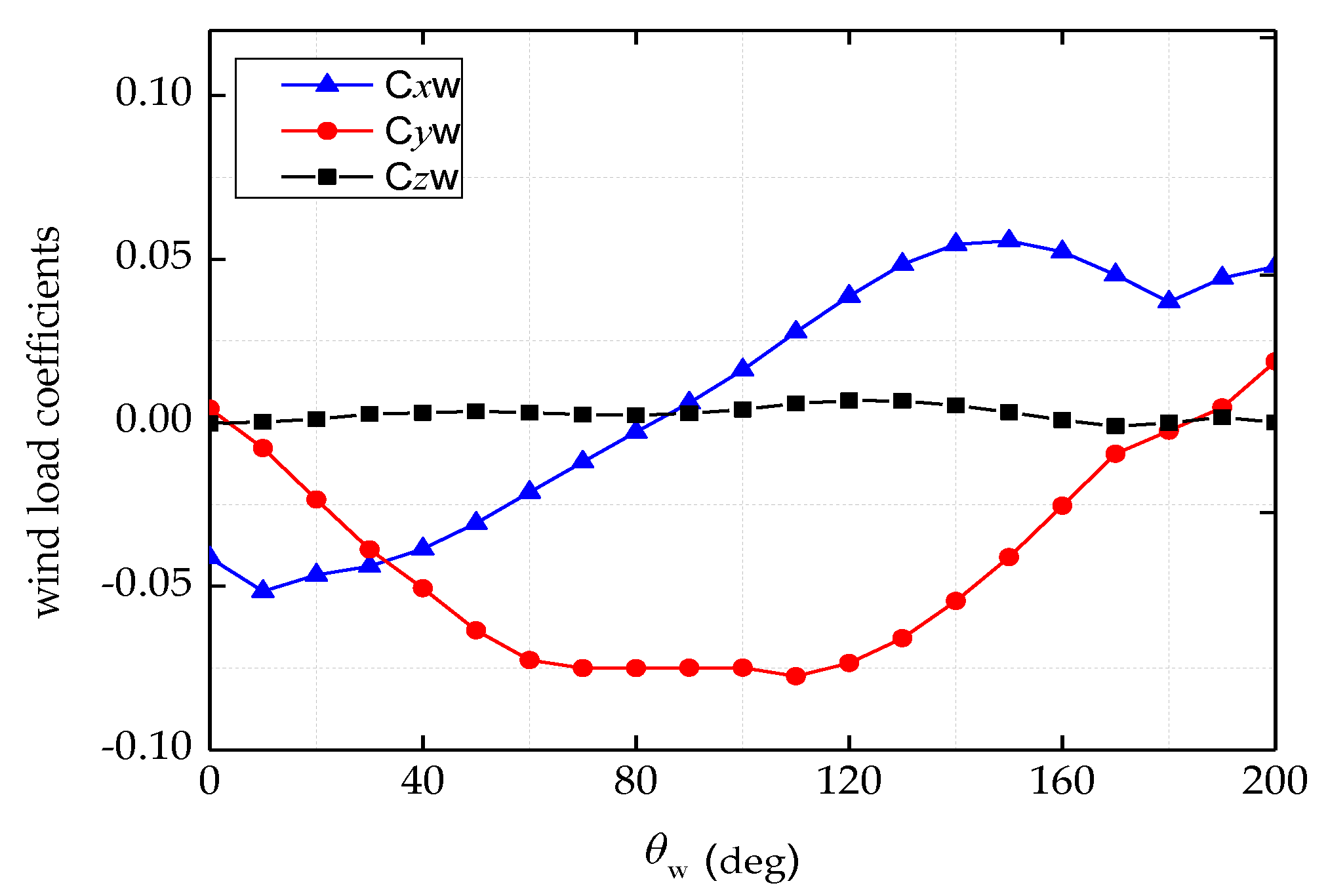
Wind, second-order wave, and current loads in the surge, sway, and yaw directions are defined as follows:

$$\begin{array}{c}{\mathsf{\tau }}_{\mathrm{wind}}={\left(\begin{array}{ccc}0.5C_{x\mathrm{w}}({\theta }_{\mathrm{w}}){\rho }_{\mathrm{a}}{V}_{\mathrm{w}}^2{L}^2,& 0.5C_{y\mathrm{w}}({\theta }_{\mathrm{w}}){\rho }_{\mathrm{a}}{V}_{\mathrm{w}}^2{L}^2,& 0.5C_{n\mathrm{w}}({\theta }_{\mathrm{w}}){\rho }_{\mathrm{a}}{V}_{\mathrm{w}}^2{L}^3\end{array}\right)}^{\mathrm{T}}\\ {\mathsf{\tau }}_{\mathrm{cu}}={\left(\begin{array}{ccc}0.5C_{x\mathrm{c}}({\theta }_{\mathrm{c}}){\rho }_{\mathrm{w}}{V}_{\mathrm{c}}^2{L}^2,& 0.5C_{y\mathrm{c}}({\theta }_{\mathrm{c}}){\rho }_{\mathrm{w}}{V}_{\mathrm{c}}^2{L}^2,& 0.5C_{n\mathrm{c}}{\rho }_{\mathrm{w}}({\theta }_{\mathrm{c}})V_{\mathrm{c}}^2{L}^3\end{array}\right)}^{\mathrm{T}}\\ {\mathsf{\tau }}_{\mathrm{wave}}={\left(\begin{array}{ccc}2{\displaystyle \underset{0}{\overset{\infty }{\int }}S(\omega )C_{x\mathrm{wa}}({\theta }_{\mathrm{wa}},\omega )\mathrm{d}\omega ,}& 2{\displaystyle \underset{0}{\overset{\infty }{\int }}S(\omega )C_{y\mathrm{wa}}({\theta }_{\mathrm{wa}},\omega )\mathrm{d}\omega },& 2{\displaystyle \underset{0}{\overset{\infty }{\int }}S(\omega )C_{n\mathrm{wa}}({\theta }_{\mathrm{wa}},\omega )\mathrm{d}\omega }\end{array}\right)}^{\mathrm{T}}\end{array}$$

(45)

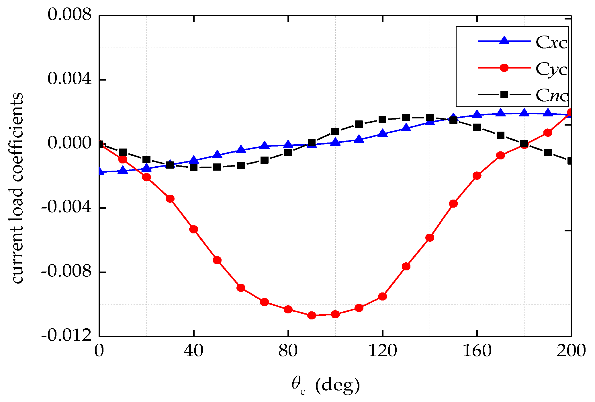
where $L$ denotes the overall length of the ship, ${\rho }_{\mathrm{a}}$ is the air density, and $V_{\mathrm{w}}$ is the wind speed. The non-dimensional wind load coefficients $C_{x\mathrm{w}}$, $C_{y\mathrm{w}}$, and $C_{n\mathrm{w}}$ are functions of the relative wind direction ${\theta }_{\mathrm{w}}$. ${\rho }_{\mathrm{w}}$ and $V_{\mathrm{c}}$ are the water density and the current speed, respectively. The non-dimensional current load coefficients $C_{x\mathrm{c}}$, $C_{y\mathrm{c}}$, and $C_{n\mathrm{c}}$ are functions of the relative current direction ${\theta }_{\mathrm{c}}$. 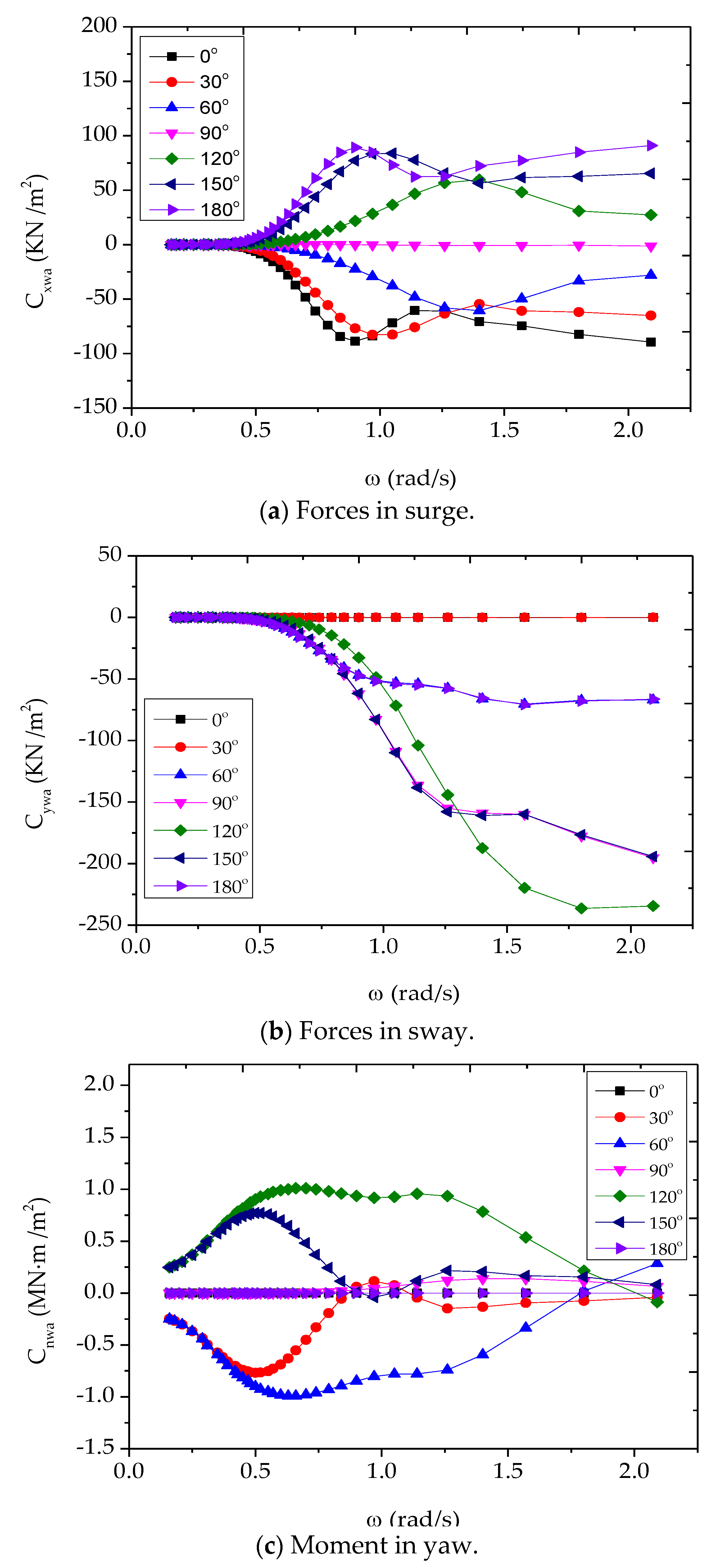$S(\omega )$ is the wave spectral density function, and $\omega$ is the wave frequency. The second-order wave force transfer functions $C_{x\mathrm{wa}}$, $C_{y\mathrm{wa}}$, and $C_{n\mathrm{wa}}$ are functions of relative wave direction ${\theta }_{\mathrm{wa}}$ and wave frequency $\omega$.

Wind and current load coefficients were obtained by a wind tunnel test in CSSRC. Second-order wave force transfer functions were obtained by numerical calculation using the software Advanced Quantitative Wave Analysis (AQWA). The results are shown in Figure 5, Figure 6 and Figure 7.

The desired position and heading were set as ${\eta }_{\mathrm{d}}={[10\mathrm{m},10\mathrm{m},{10}^{\circ }]}^T$. The initial states $\eta (0)={[20\mathrm{m},20\mathrm{m},0\mathrm{deg}]}^T$, $v(0)={[0\mathrm{m}/\mathrm{s},0\mathrm{m}/\mathrm{s},0\mathrm{deg}/\mathrm{s}]}^T$, $\xi (0)={[0,0,0]}^T$, and $\chi (0)={[0,0,0]}^T$ were selected.

In a simulation, the design parameters $K_i ,i=0,1,2$ should be large in order to speed up the convergence rate; however, parameters that are too large will cause great fluctuation. The design parameters ${\epsilon }_0$, ${\epsilon }_1$, ${\epsilon }_2$, and $\lambda$ cannot be too large, because they play an important role when the errors are close to equilibrium. The parameter $\rho$ should satisfy $0<\rho <1$, and its adjustment method is the same as that of $r$, as shown in Remark 3.

Therefore, the disturbance observer parameters were chosen as

$L_{\mathrm{d}}={(1.3\times {10}^4,0.2\times {10}^4,{10}^4)}^T$, ${\epsilon }_0=8I_{3\times 3}$, and $r=0.6$.

The adaption update law parameter was chosen as $K_0=1.5I_{3\times 3}$.

The controller parameters were selected as $K_1=\mathrm{diag}(0.055,0.045,0.035)$, ${\epsilon }_1=0.01I_{3\times 3}$, $K_2=\mathrm{diag}(0.031,0.023,0.035)$, ${\epsilon }_2=\mathrm{diag}(0.03,0.03,0.012)$, $\lambda =0.05I_{3\times 3}$, and $\rho =0.8$.

The following simulations are performed in two parts. In Section 4.1, the performance of the developed finite-time control law and the effectiveness of the designed disturbance observer are specifically evaluated, and the advantages of the ADO for unknown environmental disturbances are verified. In Section 4.2, we evaluate the performance of the proposed controller with the ADO and the auxiliary dynamic system for the cable laying ship, subject to unknown environmental disturbances and actuator saturation.

4.1. DP System with Environmental Disturbance

Here, we assume that the control law is executed completely; that is, ${\tau }_T={\tau }_c$ and ${\tilde{e}}_v=e_v$. As such, the simplified finite-time control (SFTC) law is given by

$$\begin{array}{l}{\tau }_c={\tau }_0+{\tau }_1\\ {\tau }_0=-M{K}_2{s}_v-M{\epsilon }_2{\mathrm{sgn}}^r(s_v)\\ {\tau }_1=Dv-\widehat{d}+M[\dot{\varphi }-\lambda {\mathrm{sgn}}^{\rho }(e_v)]-\Theta e_{\eta }^{T}J(\psi )e_v\end{array}$$

(46)

In order to illustrate the performance of the SFTC scheme, a simulation comparison is presented by applying the nonsingular integral terminal sliding mode (NITSM) surface in [10], where the NITSM control law is given by:

$$\begin{array}{l}{\tau }_c=Dv+M\dot{\varphi }+{\tau }_s-\widehat{d}\\ M^{-1}{\dot{\mathit{\tau }}}_s=-k_1\sigma -k_2\mathrm{sgn}(\sigma )-k_3({\dot{\mathit{e}}}_v+k_4{\mathit{e}}_v)-k_4{\dot{\mathit{e}}}_v\end{array}$$

(47)

where $\sigma ={\dot{\mathit{e}}}_v+k_4{\mathit{e}}_v+k_3{\displaystyle {\int }_0^t({\dot{\mathit{e}}}_v+k_4{e}_v})d\tau +s_{do}$. A detailed description of this control law can be found in [10]. The design matrices satisfy $k_i>0,i=1,\cdots ,4$; in simulation, the control gain $k_1$ should be increased to ensure the desired convergence speed of the system. Correspondingly, the control gain $k_2$ of the switching function needs to be as small as possible to ensure chattering reduction; however, a $k_2$ value that is too small cannot guarantee a fast convergence rate of the state when the system is close to a steady state. Therefore, the control parameters were selected as $k_1=0.1I_{3\times 3}$, $k_2={10}^{-3}{I}_{3\times 3}$, $k_1=0.1I_{3\times 3}$, $k_4=\mathrm{diag}(1,1,1)$.

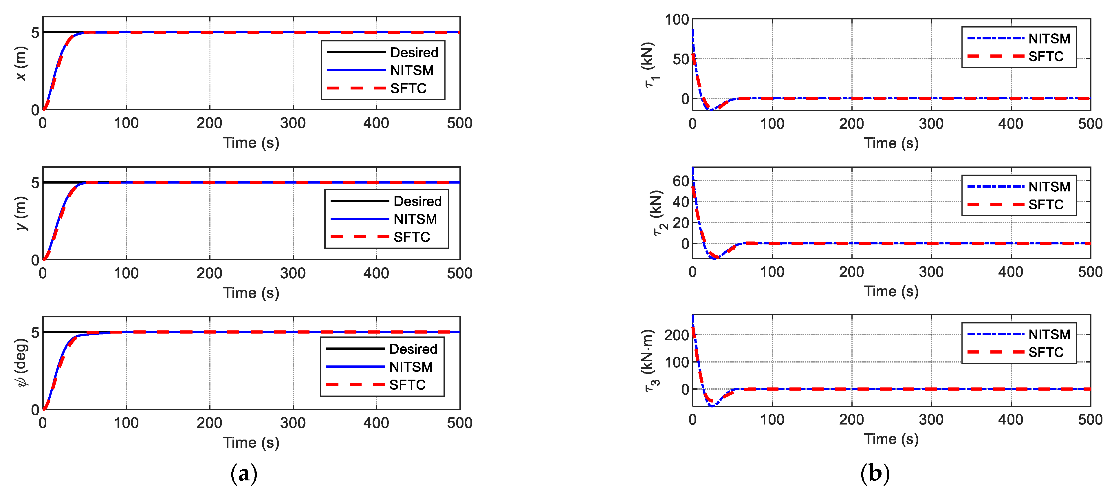
First, considering the ship DP without environmental action, i.e., $\widehat{d}=0$, the comparison of the desired and actual position and heading of the ship are shown in Figure 8a. It is obvious that both control schemes have satisfactory control performance, and the position and heading can track the predetermined trajectories at a fast convergence rate. Moreover, the control inputs, as shown in Figure 8b, are all smooth, and the control inputs of the proposed SFTC scheme are much smaller than those of the NITSM control scheme.

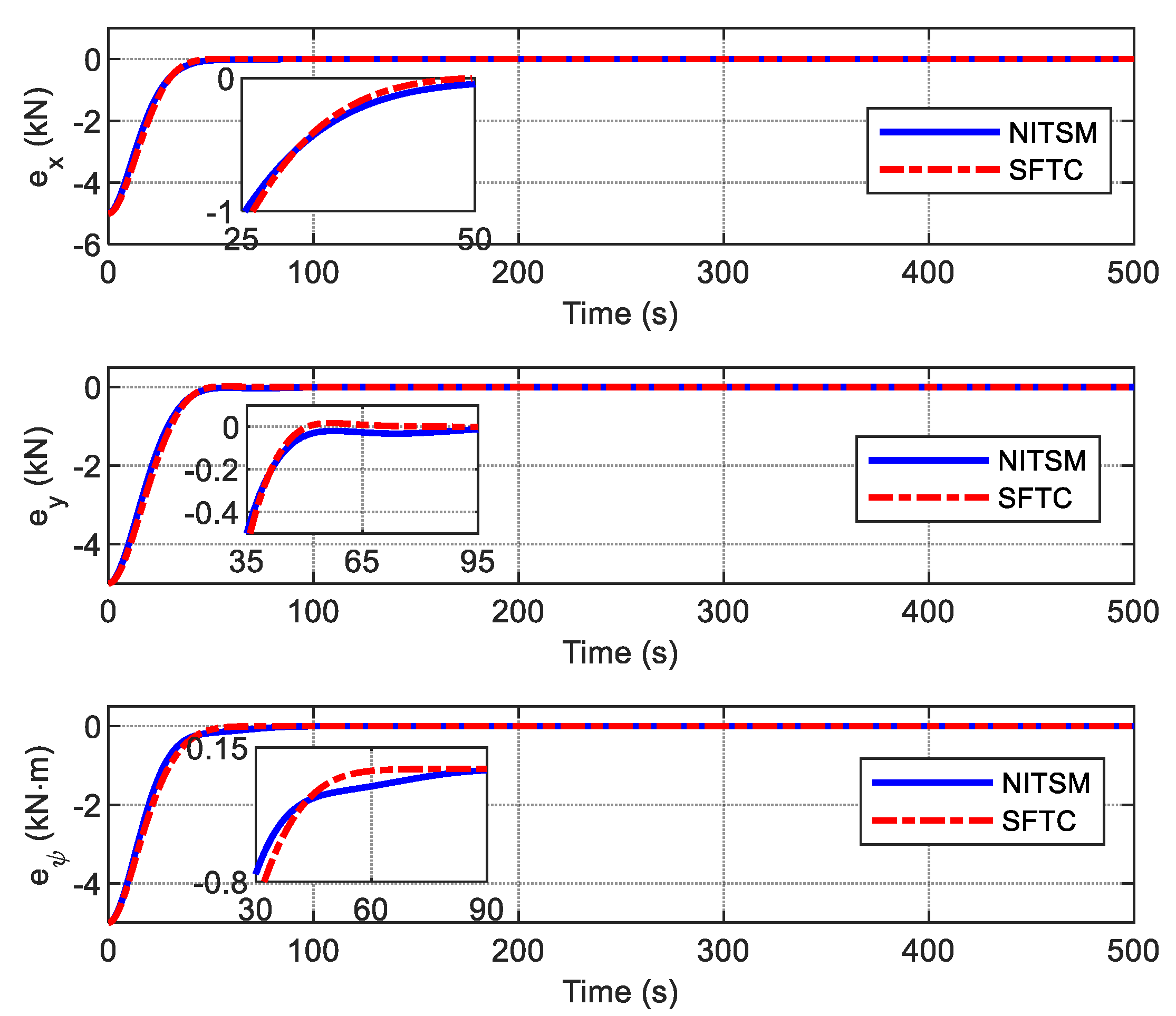
In order to better observe the dynamic response of trajectory tracking, time responses for the tracking errors are given in Figure 9; this shows that the tracking errors converge to zero in finite time for the proposed SFTC scheme and the NITSM control scheme in [10]. In the first 30 s, the convergence rate of tracking errors for the proposed SFTC scheme is slower than that of the NITSM control scheme, but as time progresses, it is obvious that the convergence rate for the SFTC scheme becomes faster. The reason for this is that the SFTC scheme with the exponential item can guarantee a fast convergence rate when the tracking errors are close to zero. However, the NITSM control scheme adopts a switching function approach law. Thus, if the tracking errors are required to converge to zero at a fast convergence rate, the selected design parameter $k_2$ must be large enough; however, if the $k_2$ parameter is too large, it will induce a chattering phenomenon in the control inputs. In summary, Figure 8 and Figure 9 verify that the proposed SFTC scheme achieves its aims of having a fast convergence rate and decreasing undesired chattering.

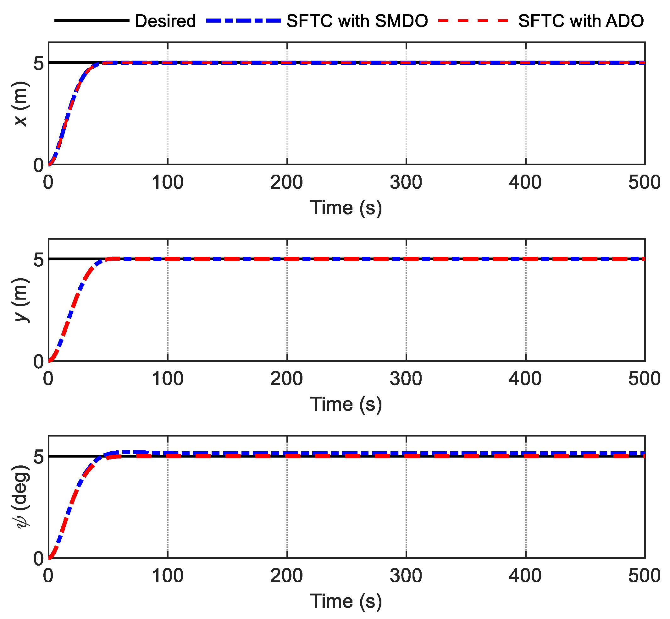
Then, taking into account the environmental parameters of Case 1, as shown in Table 2, a comparison simulation is provided to evaluate the effectiveness of the two designed disturbance observers. The positioning results for the DP system under the proposed SFTC scheme are shown in Figure 10. It is observed that the SFTC scheme with ADO achieves rapid convergence of position and heading tracking. However, the disturbance-suppression performance of the SFTC scheme with SMDO is poor; there exists significant heading-tracking steady-state errors of about 0.09 deg. This is because the upper bound value $l_3$ selected in SMDO is much smaller than the actual disturbance $d_3$, as shown in Figure 11, meaning that the environmental disturbances acting on the heading have not been effectively offset.

The estimation of disturbances via SMDO is given in Figure 11, which shows that the high-frequency-switching observed values lead to undesired chattering. As has been established, the upper bound of the environmental disturbance required for the SMDO design cannot be calculated exactly, and if the selected upper bound is too large, it will lead to the chattering of the control inputs. However, if the selected upper bound is too small, it cannot effectively compensate for the disturbances. As shown in Figure 11, it is obvious that the chosen $l_1,l_2$ values are too large to cause chattering; however, the chosen $l_3$ is too small to result in a large estimation error. All the analyses mentioned above will eventually lead to the degradation of the performance of the DP system under the SFTC scheme with SMDO, as shown by the blue dotted line in Figure 10.

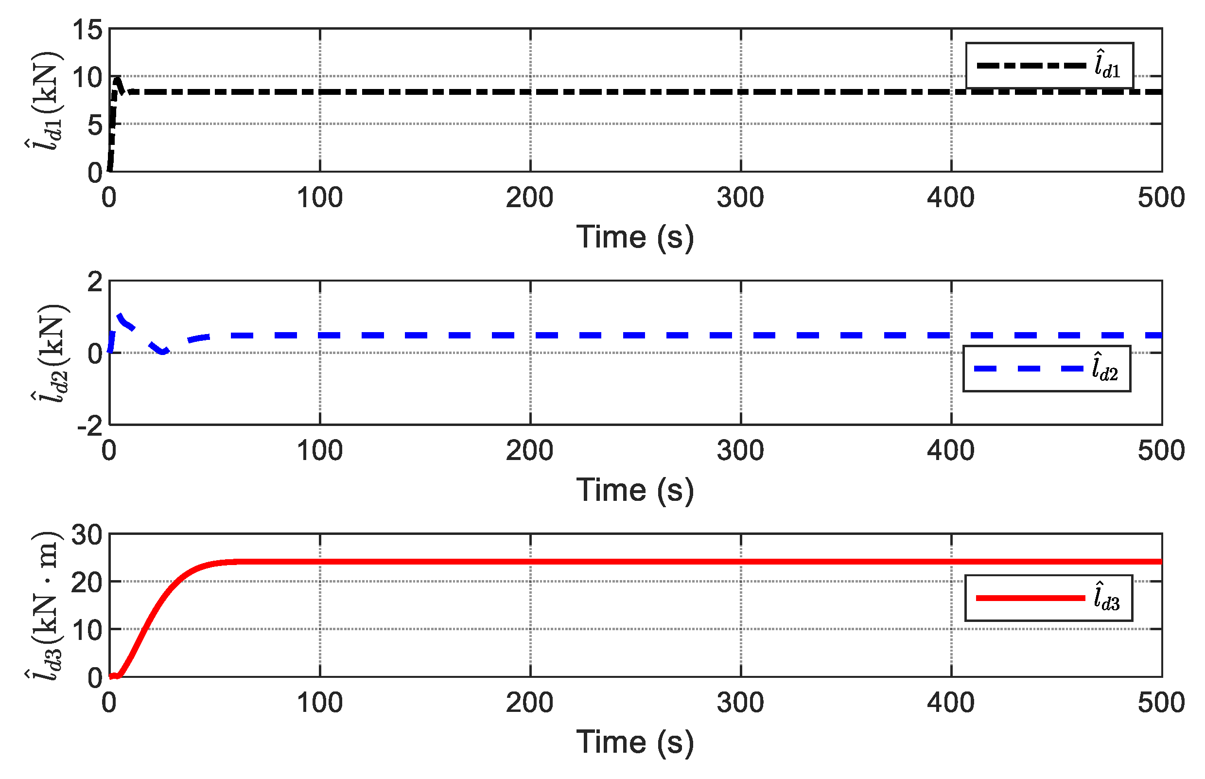
In order to eliminate the chattering, an adaptive scheme (namely, ADO) is introduced to modify the SMDO. The estimations of a disturbance generated using the ADO are shown in Figure 12, achieving a decrease in chattering compared with the results shown in Figure 11. Figure 13 shows the estimation of the upper bounds of unknown disturbances. From Figure 12 and Figure 13, it is observed that the estimation of the upper bound is highly consistent with the absolute value of the estimation of disturbances; thus, the effectiveness of the ADO is verified. The command control inputs are shown in Figure 14, which shows that the control inputs of the SFTC with ADO are much smoother than those of the SFTC with SMDO, and chattering is reduced. The above simulation results show that the proposed SFTC scheme with ADO is more effective for the DP system for ships in the presence of unknown time-varying disturbance.

4.2. DP System with Environmental Disturbances and Actuator Constraints

The objective of this subsection is to demonstrate the effectiveness of the proposed finite-time control scheme, which includes the designed ADO and the auxiliary dynamic system (29). Here, using the marine environmental parameters of Case 2, which are given in Table 2, the system’s initial states and the parameters needed for the disturbance observer and controller are all the same as mentioned above. The DP system for ships has four actuators. The designed control law is distributed into each actuator. According to whether the proposed control scheme has the ADS, the simulations are carried out in the following two cases.

For simplicity, finite-time control is noted as FTC, and auxiliary dynamic system is noted as ADS in the following simulations.

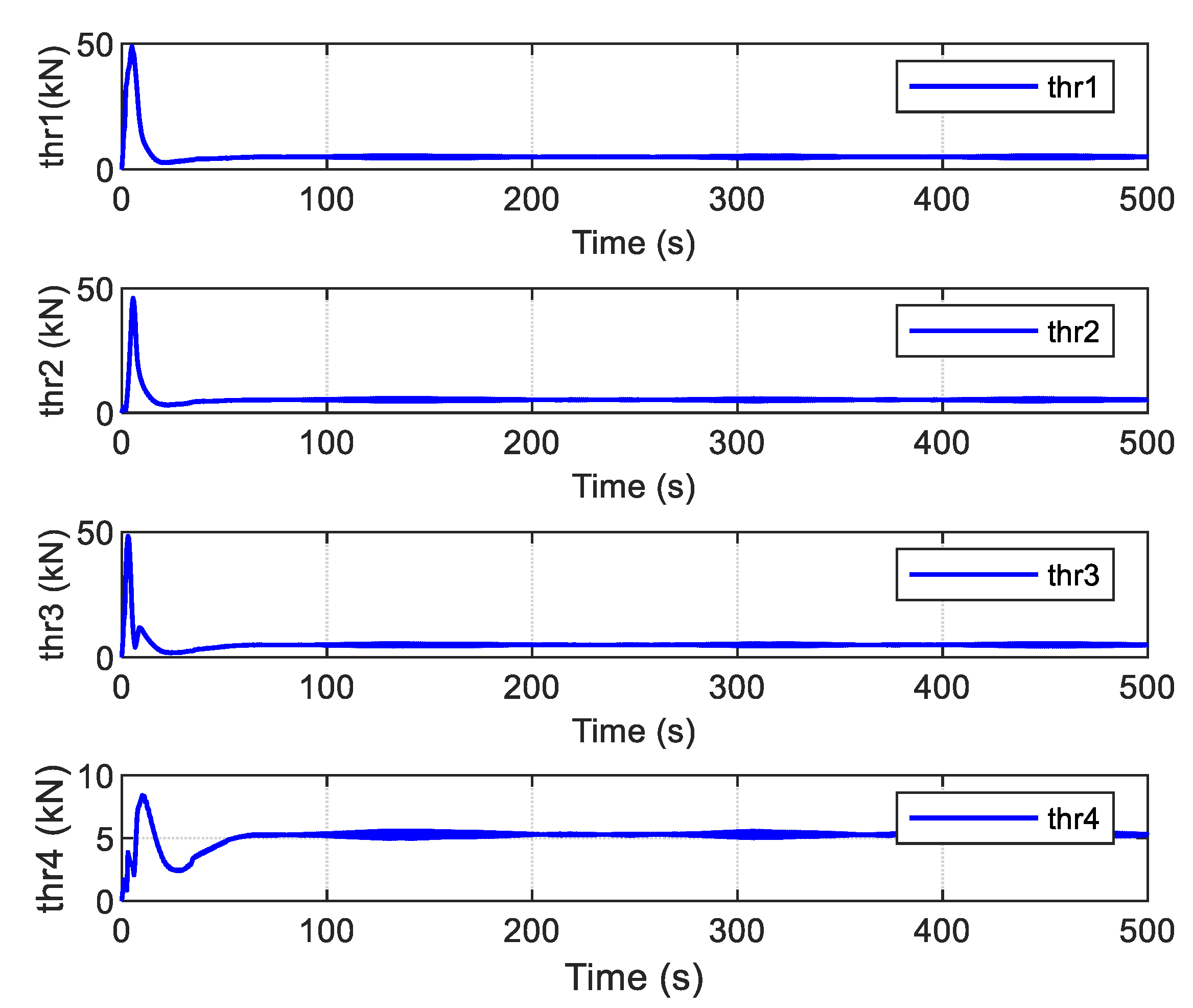
Case 1: FTC with ADO.

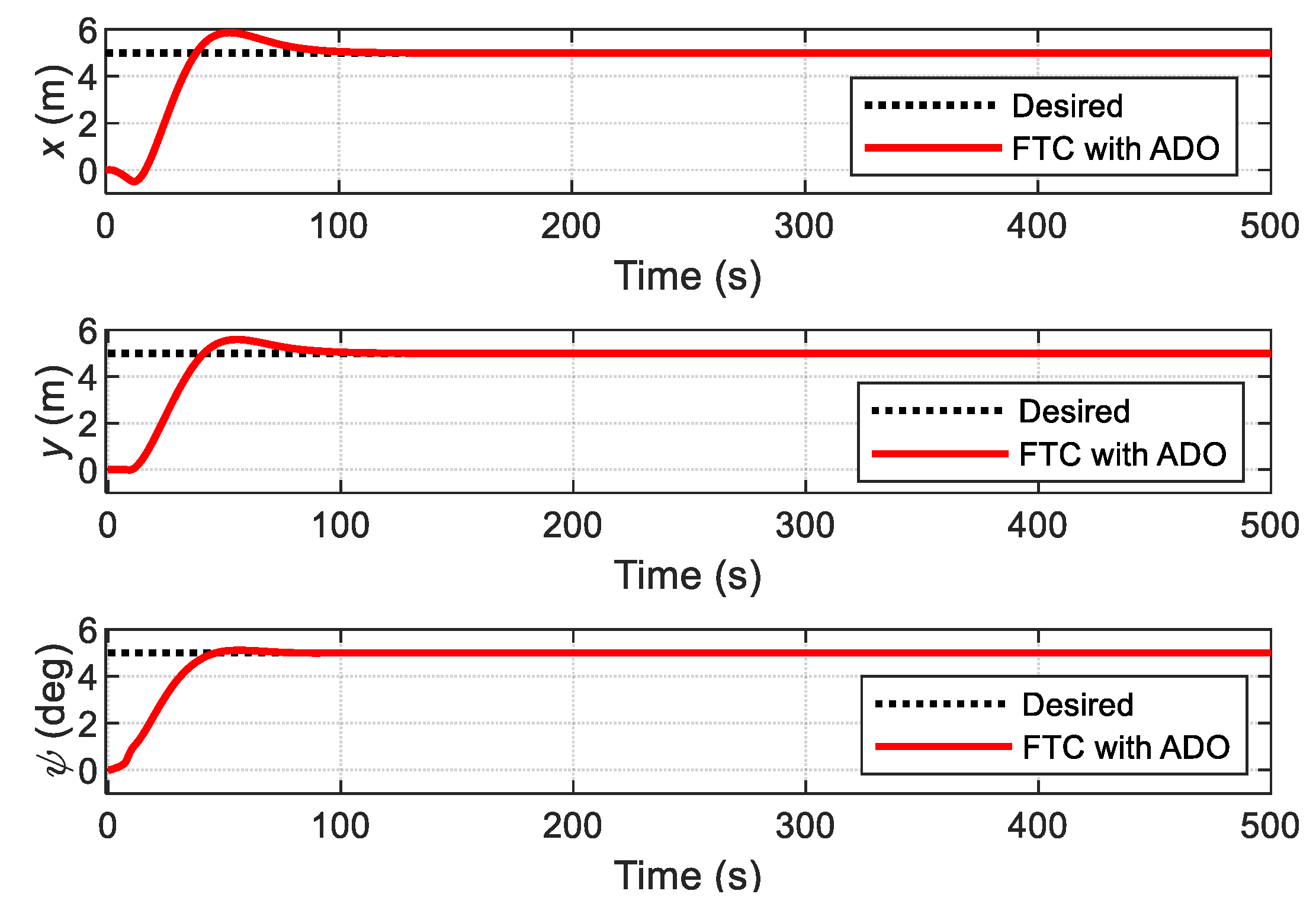
Using the proposed FTC with ADO alone, the simulation results are shown in Figure 15, Figure 16 and Figure 17. In Figure 15, it can be observed that the curves of the actual position and heading of the ship fluctuate greatly; the time taken to reach the steady state (about 100 s) is much longer than the time (about 50 s) shown by the red dotted line in Figure 10. The reason for this is that the errors between the actual and desired trajectories are too large in the initial stage; control inputs try to reduce these differences by responding quickly. However, the calculated command control inputs have not been exactly executed by the thrusters due to the physical limitations of the actuators, as shown in Figure 16. The forces of each thruster are shown in Figure 17, and it is observed that the forces required for each thruster cannot be produced due to the amplitude limitations of the turning rate of the thrusters in practice.

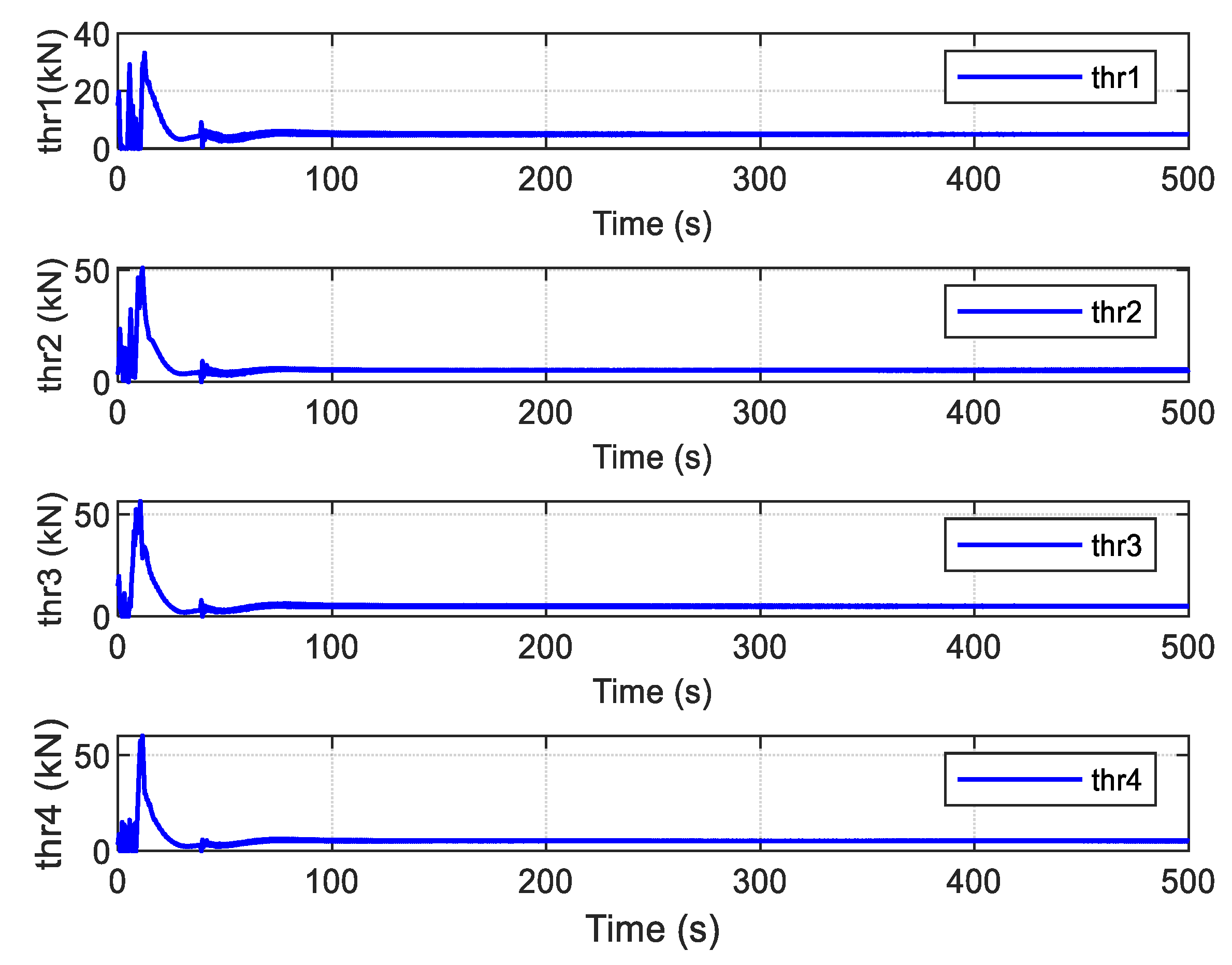
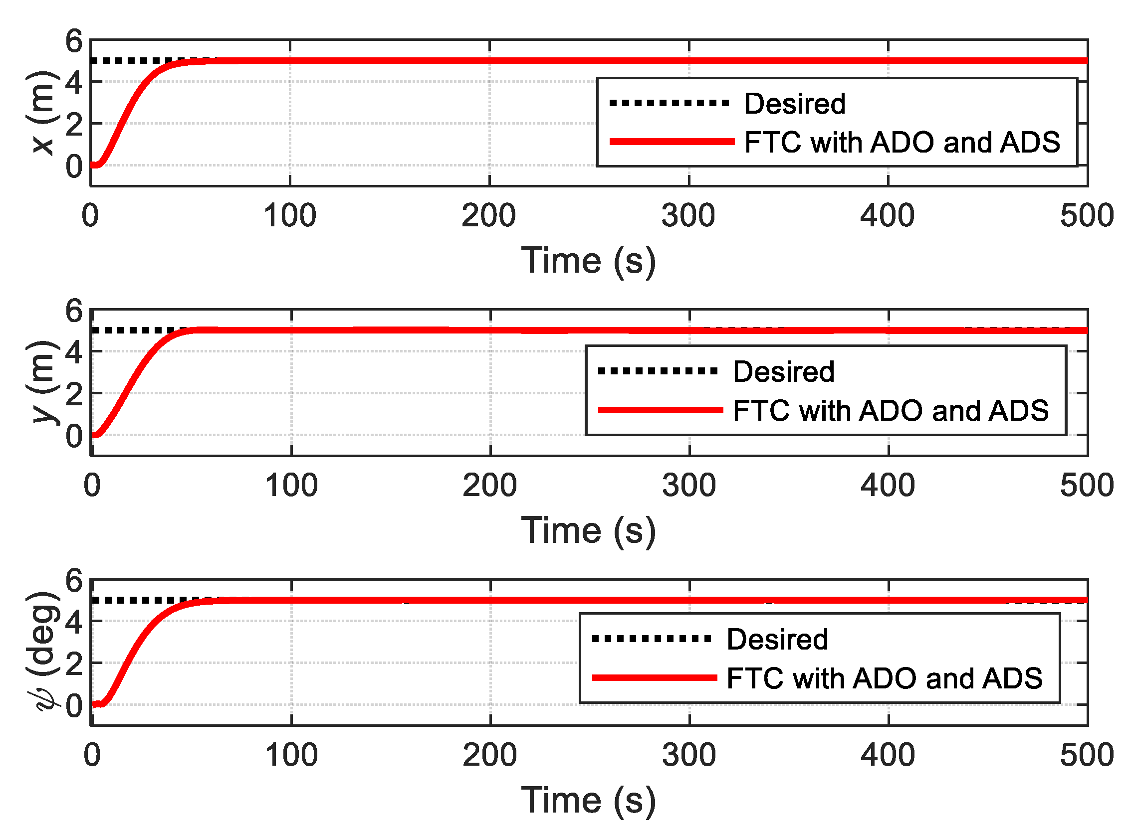
Case 2: FTC with ADO and ADS

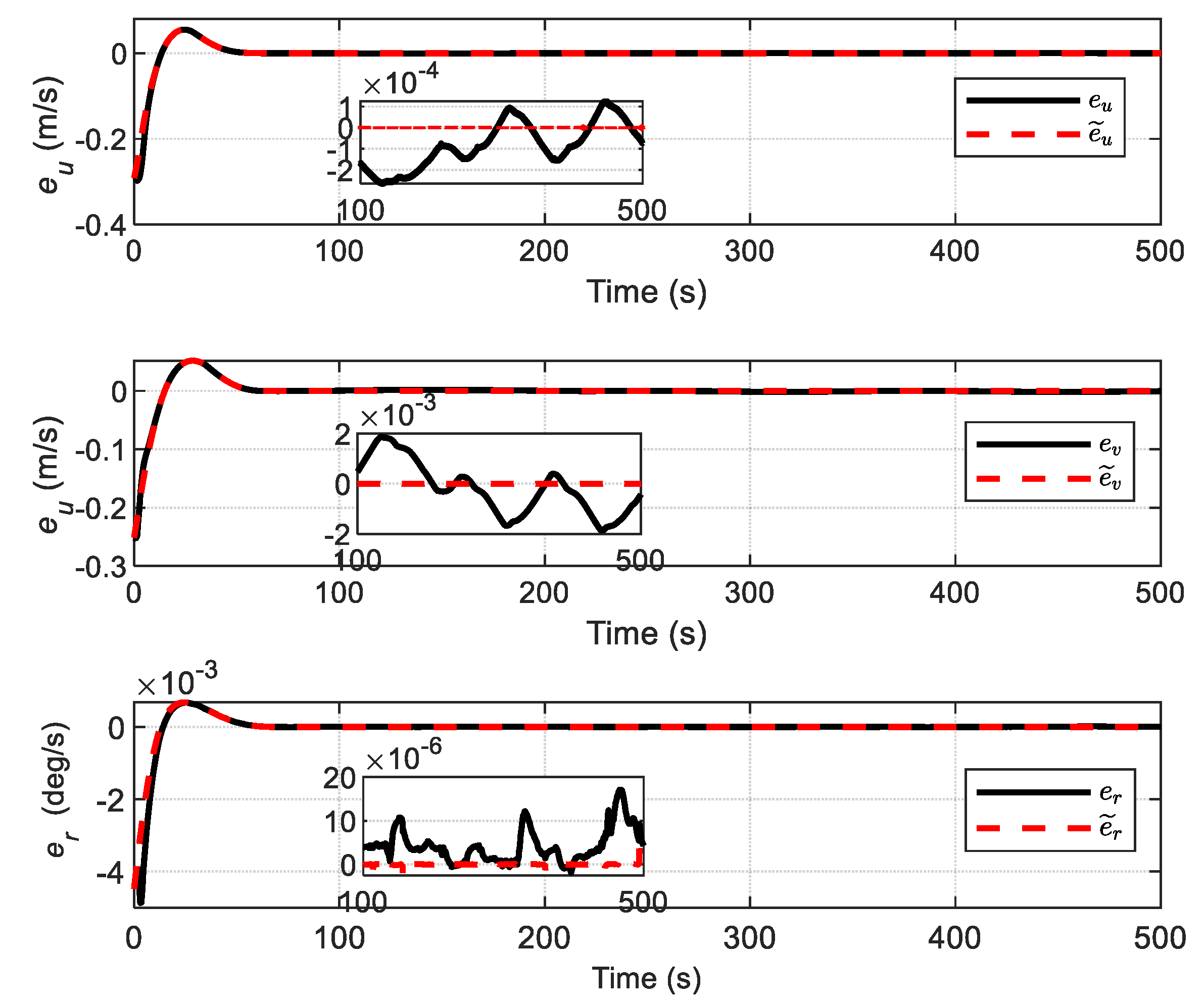
The performance of the proposed FTC with ADO and ADS is evaluated, where the ADS is applied to deal with the actuator constraints, and its design parameter is selected as $K_{\chi }=\mathrm{diag}(0.58,0.45,0.25)$. The curves of the position and heading of the ship are depicted in Figure 18; the position performance is found to be improved, in terms of convergence time, compared with that of FTC with ADO alone. Furthermore, the original velocity tracking errors $e_v$ are iteratively compensated using the ADS so that the modified velocity tracking errors ${\tilde{\mathit{e}}}_v$ are closer to zero, as shown in Figure 19. Moreover, the deviations between $e_v$ and ${\tilde{\mathit{e}}}_v$ (that is, the state vector of ADS) are bounded, and the theoretical analysis is verified.

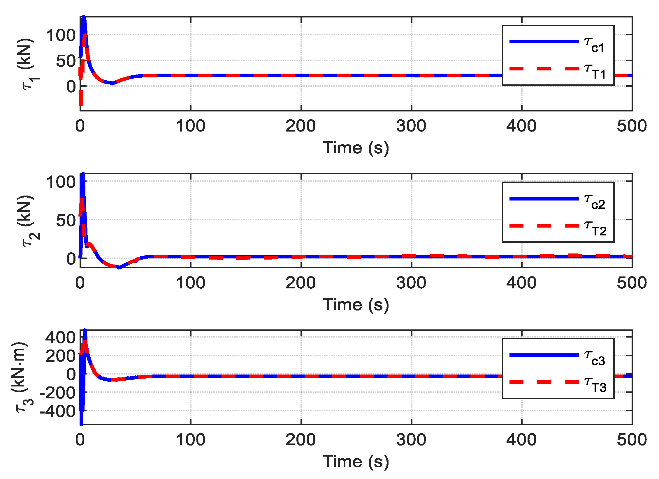
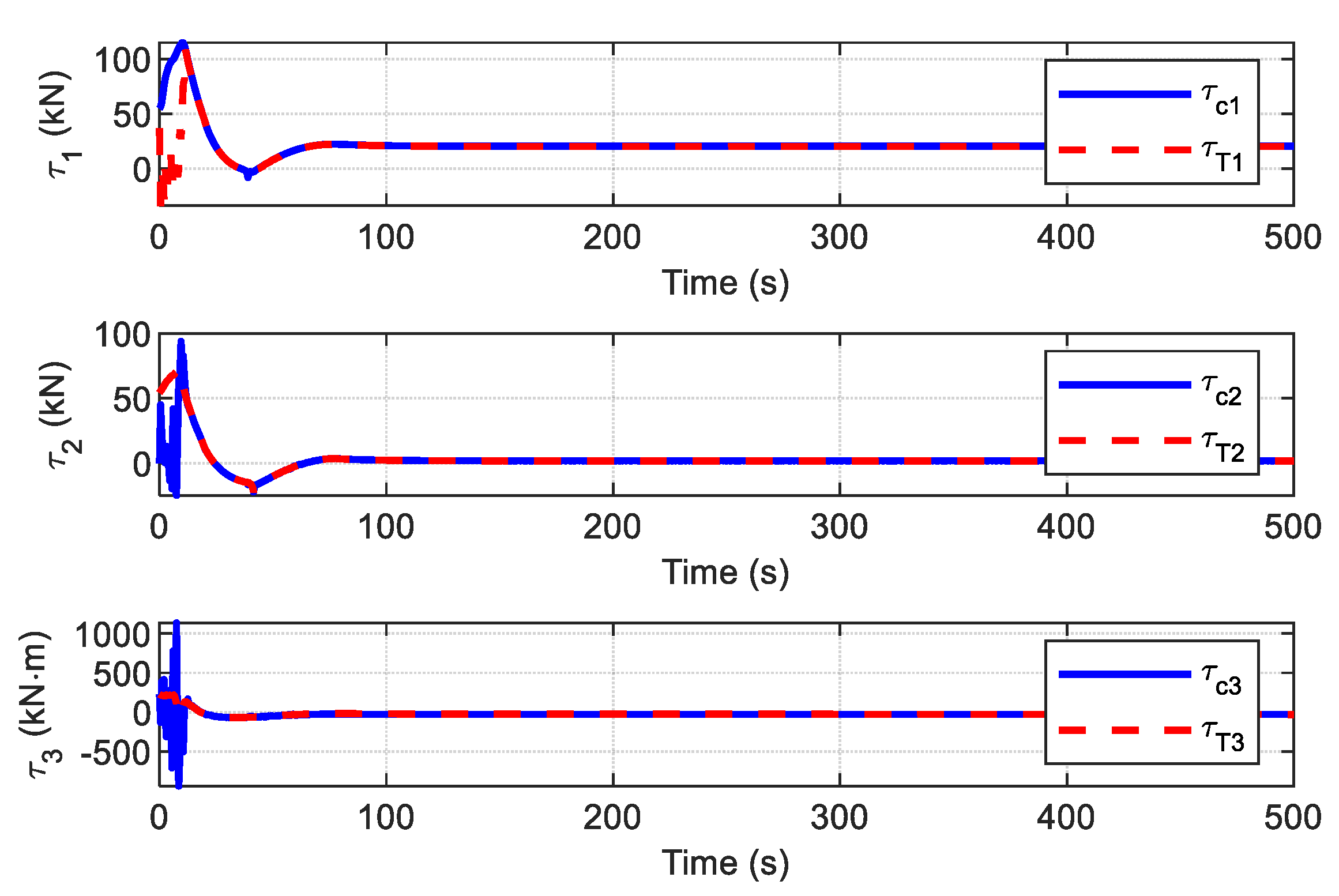
The command control law and the actual forces provided by the thrusters are shown in Figure 20. Compared with the FTC with ADO, it can be observed that the curves of the control law with the auxiliary term are much smoother in the initial stage and more easily executed by the thruster system. The forces of each thruster are given in Figure 21, which shows that iterative compensation using the auxiliary dynamic system significantly modifies the control inputs and reduces the effect of actuator saturation.

In order to quantitatively evaluate the performance of the proposed FTC with ADO and ADS, the performance indices are summarized in

Table 3. Comparison of performance indices.

Performance Indices		Control Scheme
		FTC with ADO	FTC with ADO and ADS
${\displaystyle {\int }_0^{500}|e_{\eta }(\tau )|d\tau }$	$e_x$	167	100
	$e_y$	147	107
	$e_{\psi }$	109.7	101
${\displaystyle {\int }_0^{500}\tau e_{\eta }^2(\tau )d\tau }$	$e_x$	8765	3084
	$e_y$	6596	3422
	$e_{\psi }$	3784	3720
${\displaystyle {\int }_0^{500}{\tau }_c^2(\tau )d\tau }$	${\tau }_{c1}$	$3.5\times {10}^5$	$2.6\times {10}^5$
	${\tau }_{c2}$	$6.3\times {10}^4$	$2.15\times {10}^4$
	${\tau }_{c3}$	$8\times {10}^5$	$6.1\times {10}^5$

, where the performance indices ${\displaystyle {\int }_0^t|e_{\eta }(\tau )|d\tau }$ and ${\displaystyle {\int }_0^t\tau e_{\eta }^2(\tau )d\tau }$ are used to evaluate the transient and steady-state performance of position errors, respectively. ${\displaystyle {\int }_0^t{\tau }_c^2(\tau )d\tau }$ is used to evaluate the response speed and fluctuation range of the control law. From Table 3, it can be observed that the performance indices are much lower for the proposed control technique compared with the other method mentioned in Case 1; namely, FTC with ADO. Then, by comparing the simulation results, it can be concluded that the ADS is effective for handling the actuator constraints, and the performance of the proposed FTC with ADO and ADS is superior to that of the FTC with ADO.

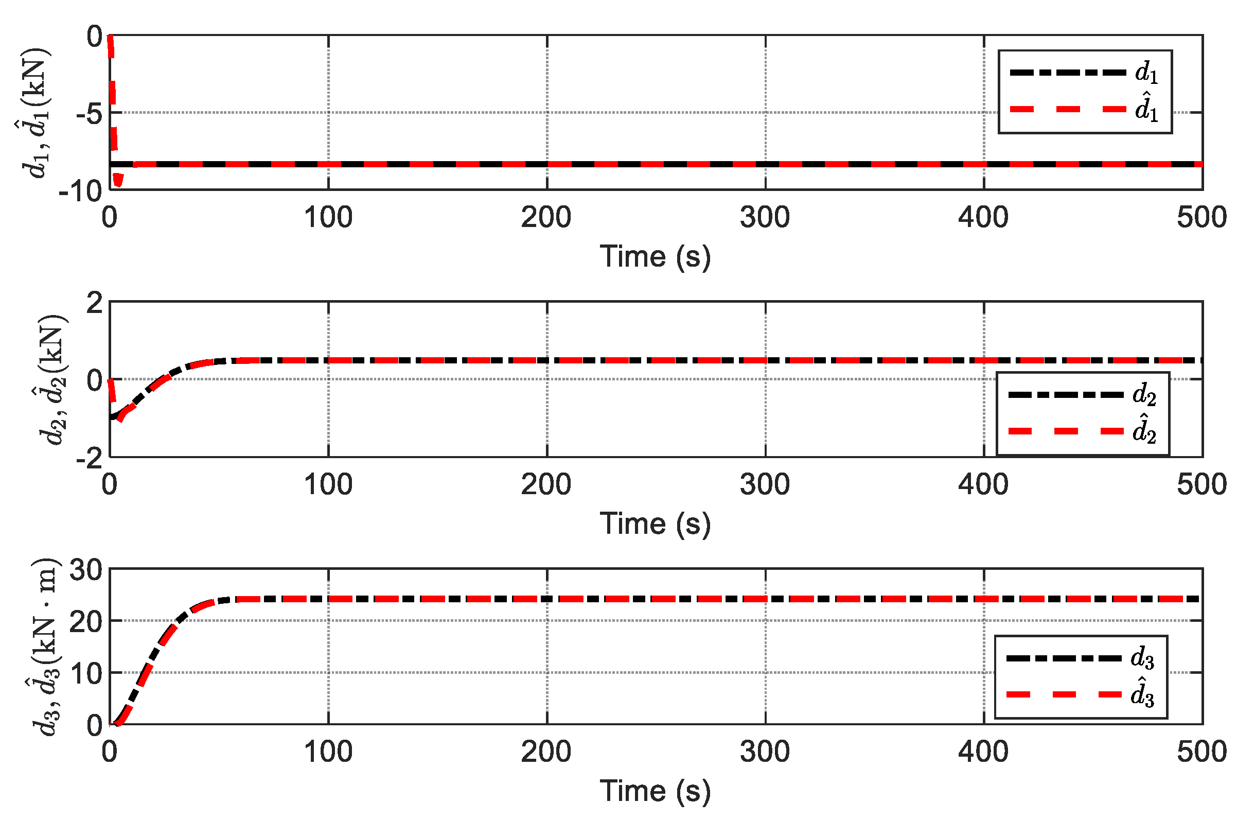
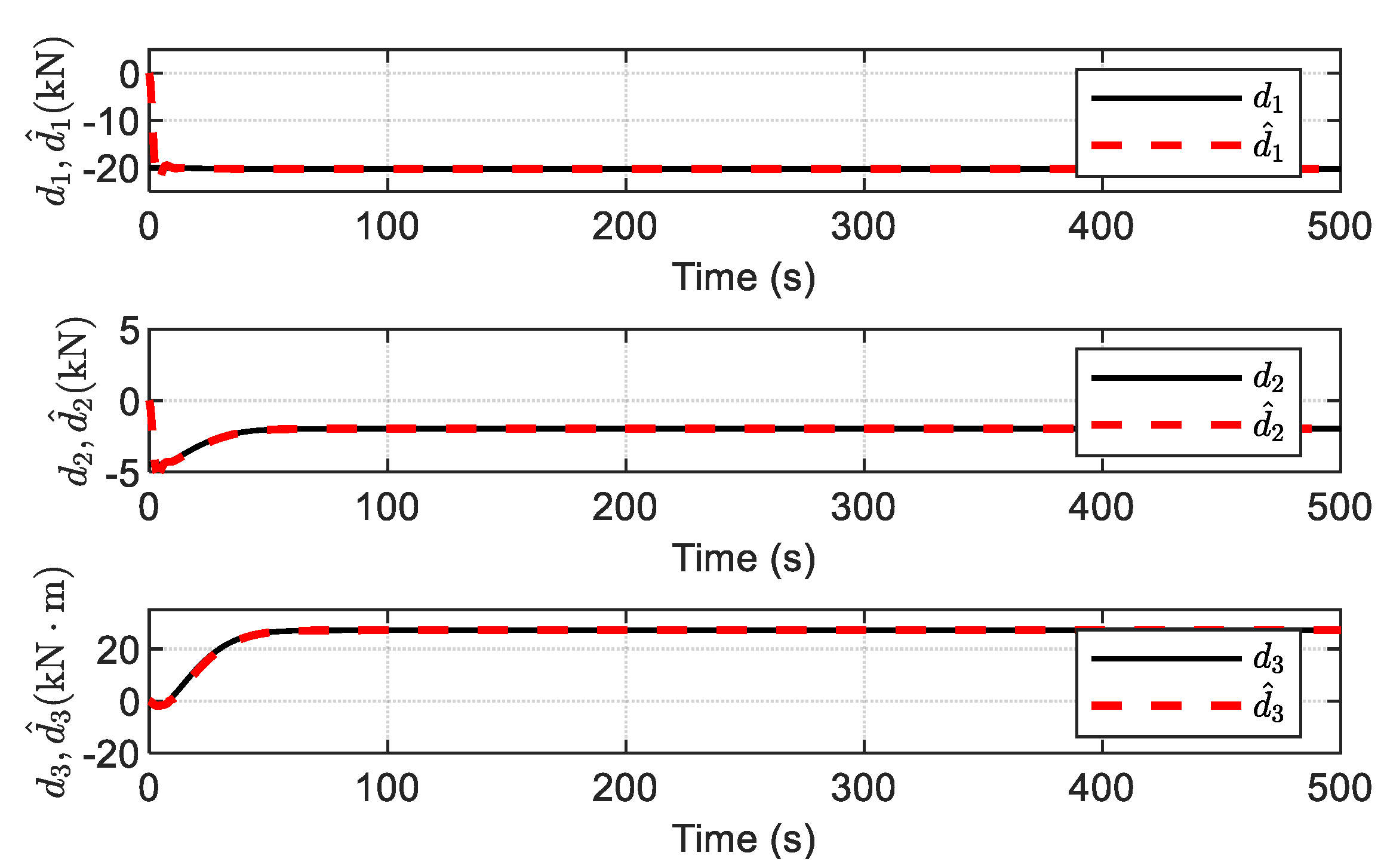
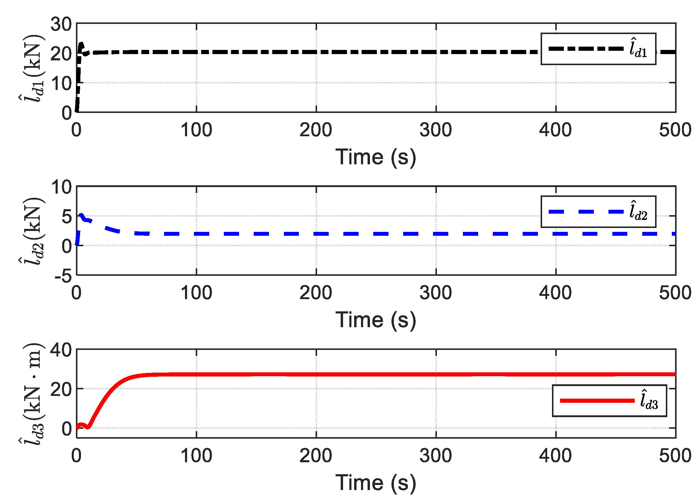
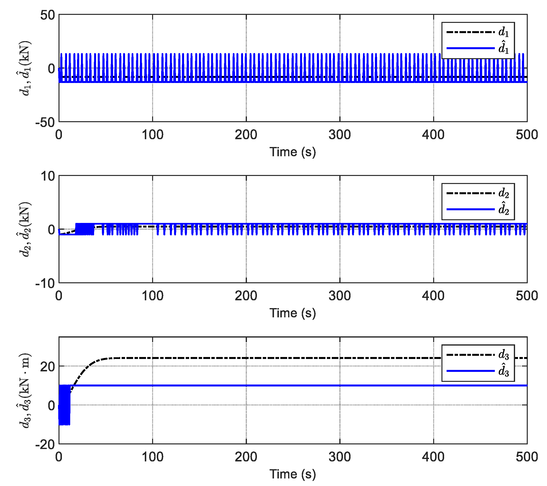
The estimation of disturbances, and the upper bound of the disturbances using the ADO, are given in Figure 22 and Figure 23, respectively. It is observed that the unknown varying-time disturbances can be accurately estimated by the ADO without readjusting its design parameters, and no prior information on the time-varying disturbances is required.

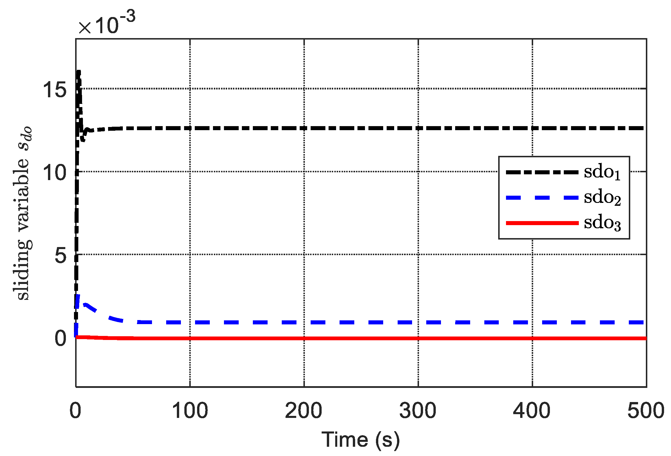
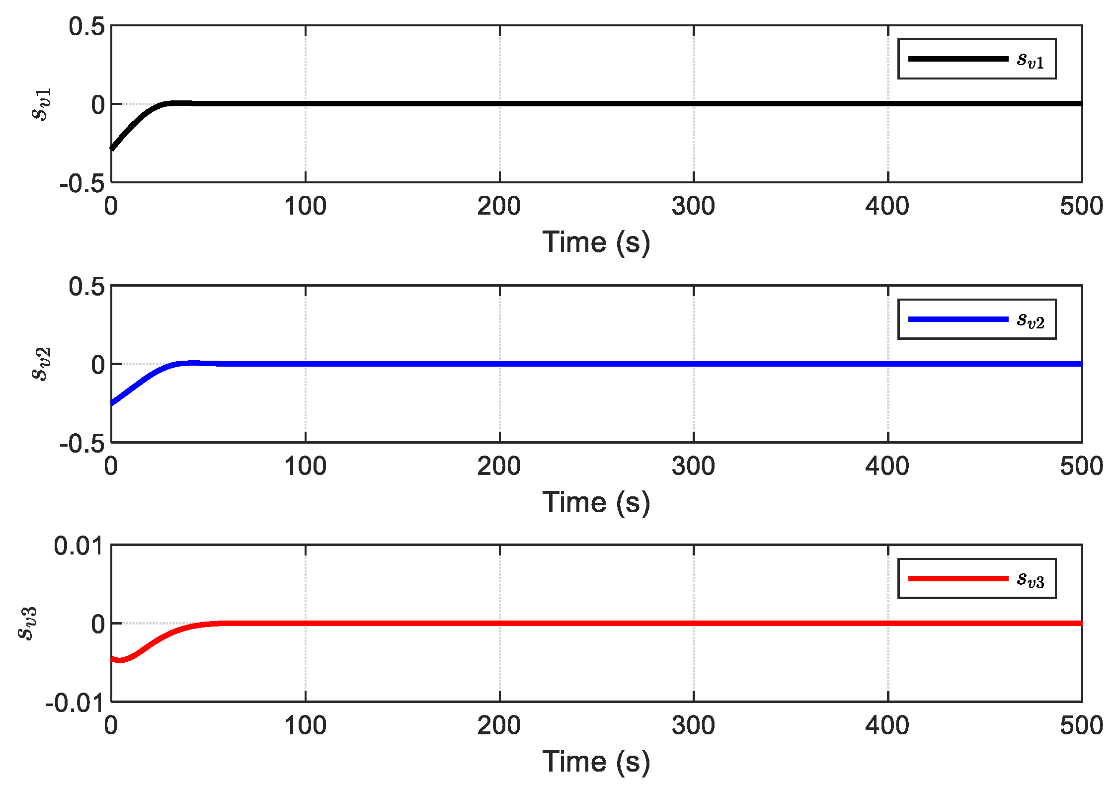
Furthermore, because the derivative of ${\overline{V}}_{do}$ is not strictly negative, the auxiliary sliding surface $s_{do}$ of the ADO is bounded and converges into a region of origin, as is demonstrated in Figure 24. The sliding surface $s_v$ is given in Figure 25, and it is observed that the sliding surface converges to zero within about 50 s. This is because the exponential reaching law guarantees that the sliding surface is reachable at high speed.

5. Conclusions

In this paper, we present the design of a finite-time control law for DP systems for ships with unknown time-varying disturbances and actuator constraints. First, to achieve disturbance suppression, the SMDO was designed to estimate the disturbances and to force the estimation errors to converge to zero in finite time. Furthermore, an ADO was presented by introducing an adaptive scheme to modify the SMDO such that undesired chattering is effectively decreased, and no prior information is required to achieve the estimate of the disturbance; however, this only guarantees the boundedness of the estimation errors. Second, to reduce the effect of actuator constraints, a joint control scheme with control allocation was presented, where the control allocation is proposed to directly inform the controller of the actuator-saturation event. The deviations of the command control inputs and the actual forces are handled using the auxiliary dynamic system. Additionally, a finite-time controller was provided, which comprises a disturbance observer and an auxiliary dynamic system, and it was proven that all closed-loop system signals are finite-time convergent. Specifically, the position tracking errors can converge to zero in finite time. Finally, numerical simulations demonstrated that the designed controller achieves the finite-time convergence of position and heading tracking and that the estimates of the ADO and the velocity errors are bounded. In the future, disturbance observers with asymptotic stability in finite time will be considered. Additionally, actuator constraints will also be considered in order to enhance the control performance of the DP system. In particular, further research will focus on how to deal with the mismatch of the DP control law and thruster forces caused by the physical limitations of the thrusters.