Predict Vessel Traffic with Weather Conditions Based on Multimodal Deep Learning

Abstract

Vessel management calls for real-time traffic flow prediction, which is difficult under complex circumstances (incidents, weather, etc.). In this paper, a multimodal learning method named Prophet-and-GRU (P&G) considering weather conditions is proposed. This model can learn both features of the long-term and interdependence of multiple inputs. There are three parts of our model: first, the Decomposing Layer uses an improved Seasonal and Trend Decomposition Using Loess (STL) based on Prophet to decompose flow data; second, the Processing Layer uses a Sequence2Sequence (S2S) module based on Gated Recurrent Units (GRU) and attention mechanism with a special mask to extract nonlinear correlation features; third, the Joint Predicting Layer produces the final prediction result. The experimental results show that the proposed model predicts traffic with an accuracy of over 90%, which outperforms advanced models. In addition, this model can trace real-time traffic flow when there is a sudden drop.

1. Introduction

Recently, the expansion of maritime traffic has driven ships and vessels towards the trend of being large-scale and specialized, which has brought pressure to the fairways and results in difficulty in vessel traffic management. Although measures such custom lanes and bidirectional lanes have been implemented, limited devices and delayed cooperation still do not satisfy the needs. As a result, vessel traffic prediction has been introduced to improve maritime traffic management. Vessel traffic prediction provides highly reliable decision support for ship navigation [1] and traffic control services [2,3].

Traffic flow is a typical case of a time series. In this field, there are a great number of studies, mainly divided into three aspects: traditional methods, shallow networks, and deep learning methods. Traditional models are also called parametric models. The most representative ones are the autoregressive integrated moving average model (ARIMA) and the Kalman filter (KF). Research has shown that the ARIMA model performed better when the dataset is small [4]. Kumur et al. [5] verified this with a seasonal-ARIMA model, achieving an accuracy of 90–96% in long-term traffic prediction. Previously, researchers did a lot of research on the Kalman filter to predict spatiotemporal sequences [6]. Abidin et al. [7] used the Kalman filter model to predict the arrival time of vehicles using Twitter information. However, these parametric models require time-to-time adjustment, which is inconvenient. To avoid this, data-driven models, also known as intelligent algorithms, have been proposed. For example, support vector machine (SVM), random forest (RF), and wavelet neural networks (WNN) are feasible for automatically modifying the parameters and creating nonlinear mapping among all dimensions of inputs. Feng et al. [8] improved SVM using multi-kernel, thereby reducing the influence of noise on the prediction results. Li et al. [9] brought SVM into spatiotemporal sequence fields by predicting the arrival time of buses based on GPS location. Other intelligent models also work well, such as support vector regression (SVR) [10], back propagation (BP) [11,12], fuzzy neural network (FNN) [13], and radial basis function network (RBFNN) [14]. However, when input dimensions are large or under uncertain influences such as a rainstorm or frigid temperatures, these methods are less likely to extract complex spatiotemporal features. Deep learning methods appear to overcome this. Krizhevsky [15] first demonstrated that a convolutional neural network (CNN) has a good effect on spatial association learning. Yu et al. [16] proposed a improved CNN using data aggregation techniques and achieved higher accuracy. The recurrent neural network (RNN) network has shown strong temporal correlation. Shi et al. [17] proposed a deep RNN model to predict household load, which is affected by some time-invariant factors. On the basis of RNN, some scholars have considered the impact of historical stream data on future prediction results, and successively proposed long short term memory networks (LSTM) [18,19,20] and GRU [21] methods, which greatly improved the prediction accuracy and lowered computational complexity. However, deep networks still show limitations in making predictions when data are complex. Some researchers then seek hybrid methods to avoid this. For example, RNN can extract the long-term feature in the sequence, whereas CNN extracts the spatial one. If combined, the hybrid model may capture both features and perform better. Shi et al. [22] took the lead in adopting the ConvLSTM model in the precipitation prediction problem, which achieved an end-to-end accurate prediction. Wang et al. [23] used a ARIMA-SVM decomposed model to predict the linear and nonlinear parts separately. Meng et al. [24] adopted a hybrid model of balanced binary tree (AVL) and k-nearest neighbor (KNN). Xie et al. [25] proposed a combined model of Bayesian network and artificial neural network. Zhang et al. [26] proposed an adaptive particle swarm optimization (PSO) method. Hu et al. [27] adopted a hybrid model of LSTM-ELM-DEA on the wind prediction problem, achieving significant performance. Zhang et al. [28] integrated four models of variational mode decomposition (VMD), self-adaptive particle swarm optimization (SAPSO), seasonal autoregressive integrated moving average (SARIMA), and deep belief network (DBN) to predict the volatility of the Spanish electricity price market.

Although vessel traffic shares many similarities with urban traffic, limited research has been conducted due to the emergence of intelligent vessel traffic (IVT). Recently both traditional and deep learning methods have been proposed. Wang [29] and Li et al. [30] realized the prediction of long-term ship flow from residual analysis and by low-rank decomposition, respectively. He et al. [31] applied an improved Kalman filter algorithm to predicting hourly traffic flow, which outperformed the regression models. It was proved that traffic flow were was not chaotic but random, and the non-parametric models may have excellent prospects [32]. Zheng et al. [33] proposed a spatiotemporal model based on deep meta-learning for the urban traffic forecasting problem, and the accuracy exceeded state-of-the-art (SOTA) methods. Wang et al. [34] adopted a hybrid model of the Prophet and WNN for prediction, which outperformed the single LSTM model. Nevertheless, the deep or hybrid methods are less than satisfactory in non-free conditions. For example, traffic flow fluctuates because of stochastic factors such as weather [35].

Most existing models use merely vessel flow data for prediction but rarely consider weather conditions such as wind, visibility, water level, and other related factors. It has been shown that extreme weather mainly poses threats to local small ships [36]. Some methods perform poorly in extreme weather conditions such as heavy rain or storms. This paper proposed a hybrid multimodal prediction model based on Prophet and GRU to tackle this problem. Weather conditions were regularized and set as inputs of this model. The Prophet framework helped decompose traffic flow sequence into components of different periods. Then Sequence2Sequence (S2S) structure was adopted to make accurate forecasts. The main contributions of this paper are listed as follows:

(1) Vessel traffic flow has some features such as long-term dependency, spatial correlation, temporal similarity, etc. One particular model may learn only one or two of them. As the core of our proposed model is a hybrid module based on Prophet and GRUs, it can learn both long-term and temporal features.

(2) Vessel traffic is often non-stationary and variable under non-free conditions due to unexpected events (accidents, collisions, weather, etc.). Weather information such as precipitation and temperature were taken as regressors to make the proposed model interpretable and robust. We verify this with experimental results based on real vessel traffic data, which indicate this model still does a good job on rainy days.

(3) The core encoder–decoder module (with attention mechanism) of the proposed model presents a stronger prediction ability in tracing real-time flow than traditional methods and other deep learning networks.

The rest of this paper is organized as follows: Section 2 presents the problem, our modeling process, and related methodologies; Section 3 illustrates the source of the dataset and the simulation results with analysis; Section 4 gives conclusions and future work.

2. Methods

2.1. Problem Definition

Vessel traffic flow prediction, especially short-term prediction, plays a key role in vessel traffic control services. Vessel traffic service (VTS) now call for digitalization and automatization [37,38,39]. For VTS operators with large areas to monitor, it is valuable to know where a traffic jam is likely to occur, which is characterized by traffic density and traffic flow volumes.

The time interval of short-term prediction is usually within an hour. Vessel traffic flow $Y_i$ is defined as mean of ships passing the observation line in the given period i; $Y\left(t\right)=[Y_0,Y_1,Y_2,\cdots ,Y_n]$ denotes history vessel traffic sequence, and $C\left(t\right)=[C_0,C_1,C_2,\cdots ,C_n]$ represents the weather sequence, including precipitation and temperature. Our task is to predict the future vessel traffic volume $Y_{n+\tau }$ at one or more steps $\tau$ based on weather data and vessel traffic data, as shown in Figure 1.

2.2. Overview of Proposed Model

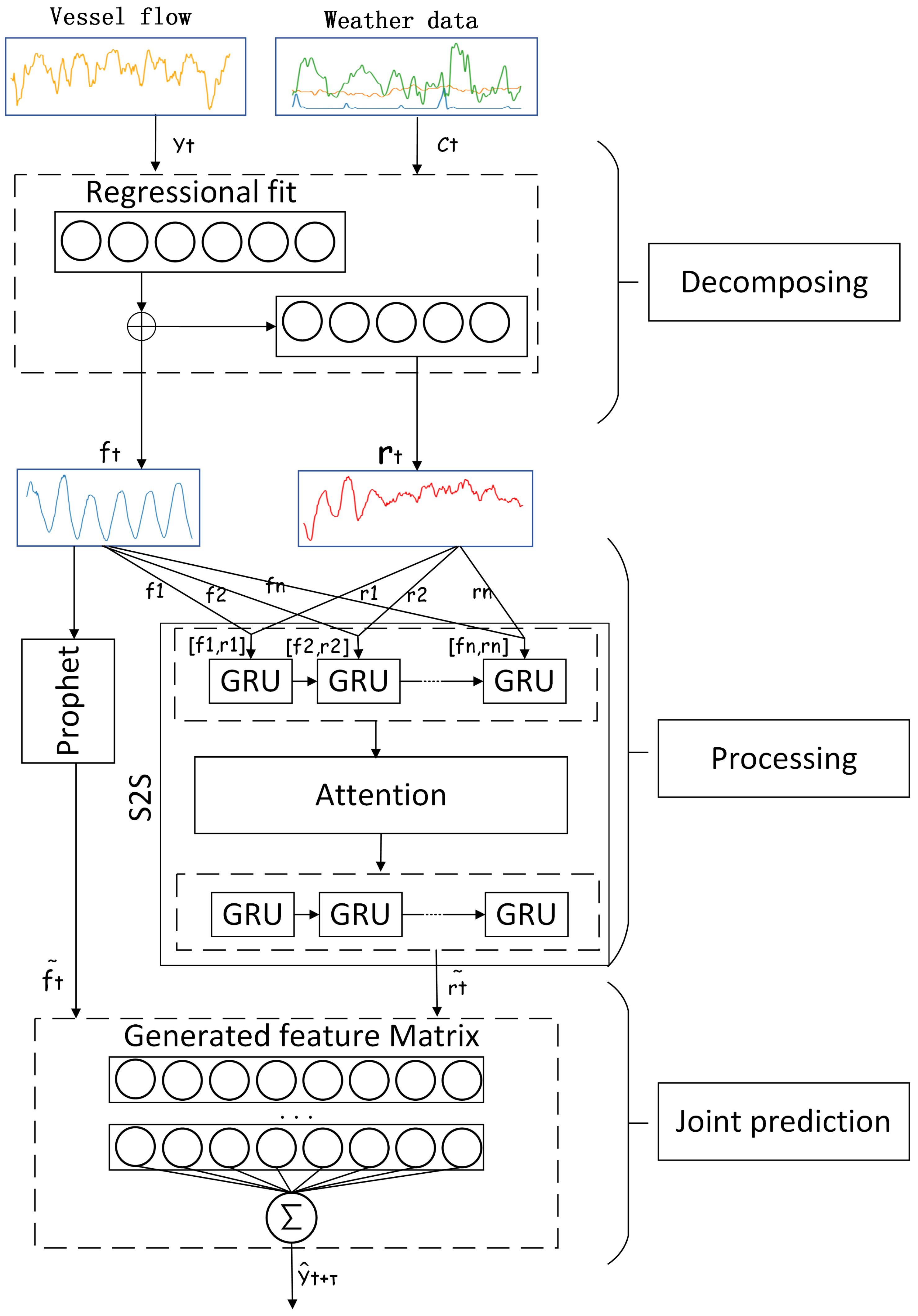
A hybrid vessel traffic prediction model on the basis of Prophet and multimodal deep learning is proposed in this paper, as shown in Figure 2. It is hierarchically composed of three layers: Decomposing Layer, Processing Layer, and Joint Prediction Layer.

Vessel traffic data and weather data are regularized and preprocessed before entering the Decomposing Layer, which divides a traffic sequence $Y_t$ into a regular component $f_t$ (contains weather features) and a residual component $r_t$. It is achieved by STL. In this process, both long-term and short-term dependency features (mainly from weather data) are considered so each component is affected mutually. Next, the two components are sent to the Prophet-S2S architecture. The Prophet part takes in the regular component only, whereas the S2S part receives both. For the S2S, GRU layers serve as the encoder, the attention mechanism as variable vector encoding, and the GRU layers again as the decoder. The next step is model fitting: we train the S2S deep learning model to extract nonlinear related features and train Prophet by multi-regression. For convenience, we adopt the Prophet module for both decomposition and processing work. The Prophet-S2S structure can handle inputs of varied dimensions and length, showing a great ability in adapting to different circumstances. Finally, the learned features are combined by the Joint Prediction Layer and densified into the final prediction results ${\widehat{Y}}_{t+\tau }$.

2.3. Prophet Framework

Prophet is an additive model for forecasting time series that was open sourced by Facebook in 2017. This model also provides a sequence decomposition method based on STL. The Prophet Framework [40] gives a decomposition formula as follows:

$$y\left(t\right)=g\left(t\right)+s\left(t\right)+h\left(t\right)+{\epsilon }_t$$

(1)

In Formula (1), time series $y\left(t\right)$ is decomposed into four parts: $g\left(t\right)$, $h\left(t\right)$, $s\left(t\right)$, and ${\epsilon }_t$, where $g\left(t\right)$ represents for the non-periodic growth term called Trend, $s\left(t\right)$ are cyclical changes named Seasonality, $h\left(t\right)$ is the impact term of non-periodic emergencies designated as Events, and ${\epsilon }_t$ is the singular term that cannot be captured. In this system, ${\epsilon }_t$ is considered as Gaussian white noise.

2.3.1. Trend

For Trend, the Prophet algorithm provides two fitting models: saturating growth and piecewise linear. The former assumes that the growth has a bearing tolerance, thus it is impossible to increase or decrease infinitely. The fitting pattern is logistic regression. The latter assumes that the model has no upper or lower volume limits. Vessel traffic flow is limited by the channel capacity and other facilities, and there seems be a theoretical ceiling. However, practice and experiments show that logistic regression fits poorly in vessel flow data due to highly nonlinear and periodic oscillations. Therefore, in this paper, piecewise linear is applied instead. The trend term for piecewise linear is calculated as follows:

$$g\left(t\right)=-k\left(t\right)(t-m(t\left)\right)$$

(2)

where $k\left(t\right)$ and $m\left(t\right)$ in Formula (2) stand for rate and offset function, respectively. Assume that rate k adjusts at times $s_j,j\in \{1,2,\cdots ,n\}$ with the initial value k. Change rate at time $s_j$ is calculated by adding all the previous change rates together, as is shown in Formula (3):

$$k\left(t\right)=k+{\sum }_{t>s_j}{\delta }_j$$

(3)

where ${\delta }_j$ denotes the rate at point j. Let $a\left(t\right)={[a_1\left(t\right),\cdots ,a_n\left(t\right)]}^T\begin{array}{cc}s.t.& aj\in \{0,1\},\end{array}$$k\left(t\right)$ is rewritten as:

$$k\left(t\right)=-(k+a{\left(t\right)}^T\delta ),\begin{array}{cc}s.t.& a_j\end{array}=\left\{\begin{array}{cc}1& t\ge s_j\\ 0& else\end{array}\right.$$

(4)

To ensure the continuity of $g\left(t\right)$, namely $\underset{t->s_j-}{lim}g\left(t\right)=g\left(t\right){|}_{t=s_j+}$, the offset function is:

$$m\left(t\right)=m+a{\left(t\right)}^T\gamma$$

(5)

Similarly, here $\gamma =[{\gamma }_1,{\gamma }_2,...,{\gamma }_n]$ and ${\gamma }_j=-s_j{\delta }_j$.

2.3.2. Seasonality

Vessel traffic flow presents multi-period seasonality as a result of regular human activities. The vessel flow curve may present periods of yearly, monthly, or weekly intervals. To find out how traffic data are influenced, we must first specify the implicit periodicity. The term Seasonality $s\left(t\right)$ in Formula (1) provides an extensible model based on Fourier transform [41]. For a certain cycle P, $s\left(t\right)$ in Fourier series is expressed as:

$$s\left(t\right)=\sum _{i=1}^N[a_{i}cos(\frac{2\pi i}{P}t)+b_{i}sin(\frac{2\pi i}{P}t)]$$

(6)

Let $X\left(t\right)=\left[cos\right(2\pi t/P),sin(2\pi t/P),\cdots ,sin(2\pi N·t/P\left)\right]$, and $\beta ={[a_1,b_1,\cdots ,b_n]}^T$; $s\left(t\right)$ is updated as follows:

$$s\left(t\right)=X\left(t\right)\beta$$

(7)

where $\beta$∼$N(0,{\sigma }^2)$.

2.3.3. Events

Events represent the impact of non-periodic factors on traffic flow, which is usually unpredictable and gradual (such as heavy rain, high temperature, etc.). These events empirically carry an impact on traffic flow, but the level stays uncertain. We assume that there are N events in the time period T, each corresponding to the period $T_i(1\le i\le N)$; $h\left(t\right)$ in Formula (1) is as follows:

$$h\left(t\right)=Z\left(t\right)\kappa$$

(8)

where

$$\begin{array}{c}Z\left(t\right)=[1(t\in T_1),0,\cdots ,1(t\in T_2),\cdots ,1(t\in T_N)]\hfill \\ \begin{array}{ccc}\begin{array}{cc}\begin{array}{ccc}& & \end{array}& \end{array}& \kappa \sim N(0,{\nu }^2)& \end{array}\hfill \end{array}$$

(9)

In this paper, events such as precipitation and temperature are regarded as multiplicative rather than additive; thereby Formula (1) is rewritten as:

$$y\left(t\right)=g\left(t\right)\ast (1+h\left(t\right))+s\left(t\right)+{\epsilon }_t$$

(10)

Note that in Figure 2, $Y_t=f_t+r_t$, where $Y_t$ denotes flow data. Some revisions for (10) are made:

$$\begin{array}{c}y\left(t\right)=f\left(t\right)+r\left(t\right)\hfill \\ \begin{array}{cc}& =\end{array}exp(g^{\prime }\left(t\right)+h^{\prime }\left(t\right))+s\left(t\right)+{\epsilon }_t\hfill \end{array}$$

(11)

where

$$\left\{\begin{array}{ccc}f\left(t\right)=exp(g^{\prime }\left(t\right)+h^{\prime }\left(t\right))& & \\ g^{\prime }\left(t\right)=ln\left(g\left(t\right)\right)& s.t.& h\left(t\right)>-1\\ h^{\prime }\left(t\right)=ln(h\left(t\right)+1)& & \end{array}\right.$$

(12)

In Formula (12), a log-and-exp operation is applied to $f\left(t\right)$ because we expect that $f\left(t\right)$ is covered within a restrained range, which is helpful for normalizing later. At the same time, multiplicative regressors are manipulated in an additive way, which enhances the calculation precision.

The revised Prophet module does not need to repeatedly estimate parameters to make adjustments and has a high tolerance for missing values, which in turn eliminates the impact of errors caused by interpolation. There are two merits of our revised version:

(1) Long-term memory capacity: The module fits quickly even for long sequences, overcoming the problem of long time learning in deep learning methods.

(2) Considering impacts of events: It is difficult for deep learning models to foresee sudden changes, whereas, to some extent, this module does.

2.4. Sequence2Sequence Architecture

2.4.1. LSTM and GRU

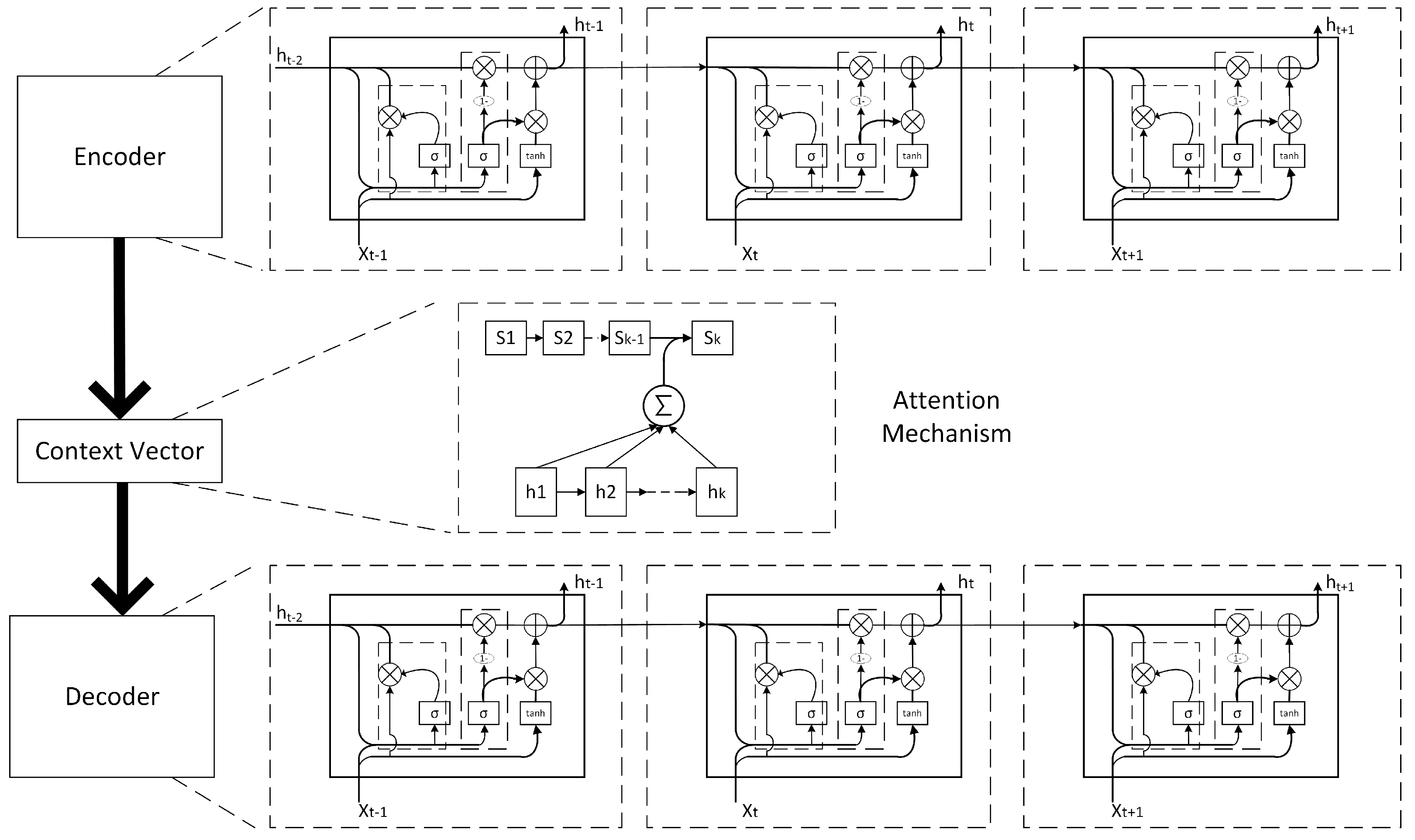
LSTM is a typical RNN. LSTM has a special memory cell that establishes long-term dependencies through three gates: input gate, output gate, and forget gate. In this way, the problems of gradients exploding and vanishing are significantly improved. In this paper, a variant of LSTM named GRU is adopted. GRU has almost the same performance as LSTM, but gets fewer parameters to update in back propagation, resulting in a faster convergence. The structures of the RNN network and GRU memory cell are shown in Figure 3:

The right side of Figure 3 shows the structure of a GRU unit. Each unit receives $X_t$ at time t and the previous unit’s state $h_{t-1}$ as inputs, where $h_t$ is the output of the current unit and will be passed to the next unit. The iteration of parameters is then completed by the reset gate and update gate, respectively. The reset gate determines the degree to which past information should be forgotten; the input gate controls the contribution of new information. All parameters are computed as:

$$\left\{\begin{array}{c}{r}_t=\sigma (W_1·h_{t-1}+V_1·X_t+b_1)\\ \stackrel{\sim }{h_t}=tanh(W_3·(r_t\ast h_{t-1})+V_3·X_t+b_3)\\ z_t=\sigma (W_2·h_{t-1}+V_2·X_t+b_2)\\ \begin{array}{c}{h}_t=(1-z_t)·h_{t-1}+z_t\ast \stackrel{\sim }{h_t})\\ y_t=\sigma (W_0·h_t)\end{array}\end{array}\right.,$$

(13)

where · denotes the Hadamard product and $\sigma$ the sigmoid function; W, V are the weight matrices, and b are the bias parameters.

2.4.2. Sequence to Sequence

Sequence to Sequence (S2S) was developed by Google and is now one of the primary methods in the field of natural language processing (NLP). Different from other encoder–decoder methods, S2S emphasizes sequence order by position encoding. In this paper, our S2S model uses GRU-Attention-GRU structure, as shown in Figure 4.

It is perplexing how short, long, or other features decide the following output. Therefore, the attention mechanism is applied to help the decoder learn weights of different units:

$$\left\{\begin{array}{c}{e}_{ij}=a(s_{i-1},h_j)\\ a_{ij}=\frac{exp\left(e_{ij}\right)}{{\sum }_{k=1}^{Tx}exp\left(e_{ik}\right)}\\ c_i={\sum }_{j=1}^{Tx}{a}_{ij}{h}_j\end{array}\right.,$$

(14)

where $e_{ij}$ represents the impact of previous outputs $h_j$ on present state $s_i$. A softmax-normalization is applied to get the distribution of $a_{ij}$, which indicates the degree of significance of time j to i. The weighted sum of $h_j$ produces context vector $c_i$.

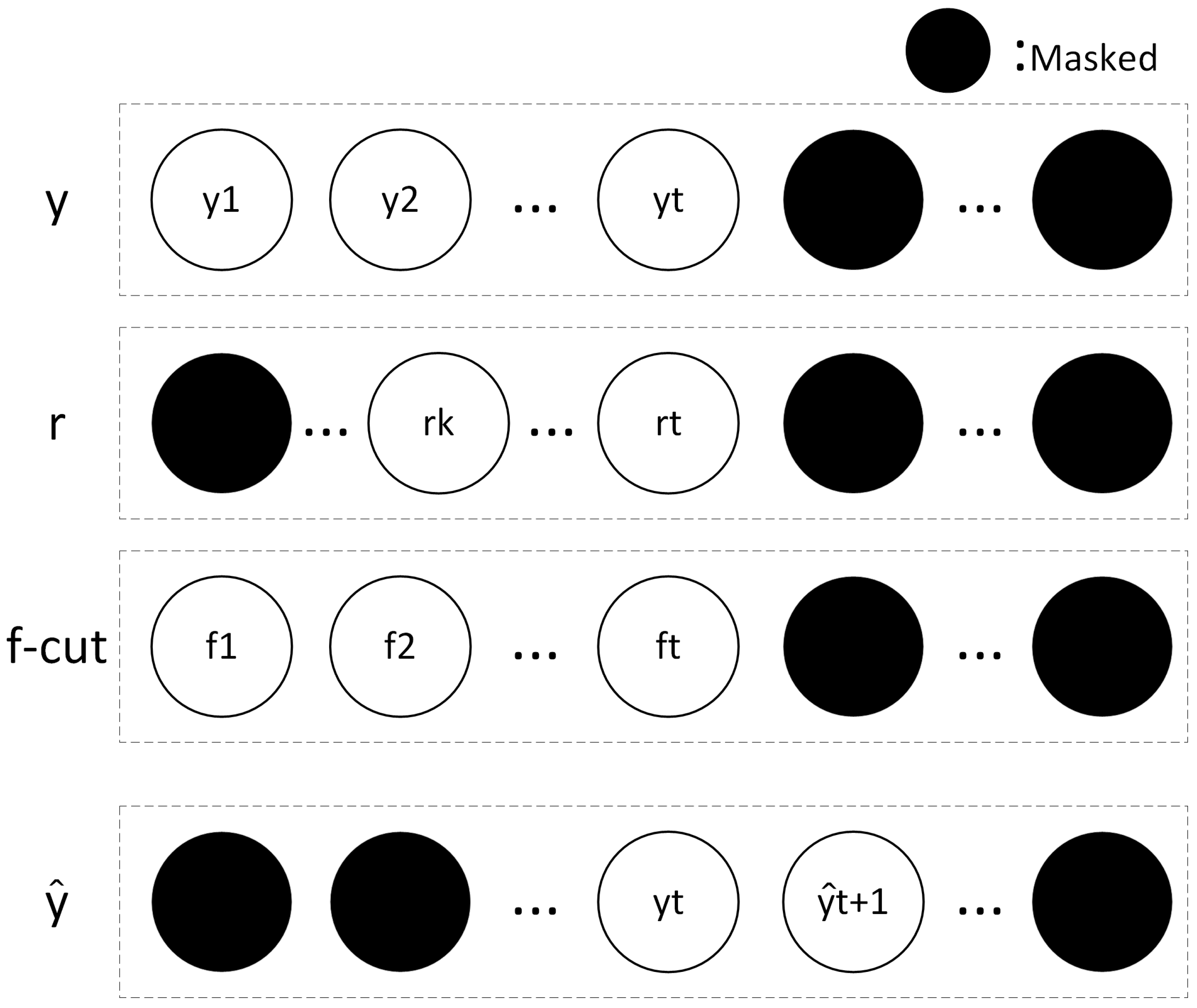
To construct the feature matrix, $f\left(t\right)$ from Formula (11) is cut off by a sliding window. Then, the truncated $f\left(t\right)$ and $r\left(t\right)$ form the input of S2S. As Prophet receives a long sequence while the S2S gets a relatively shorter one, this may lead to a problem called information leakage (the inputs “know” information of outputs ahead of time). In this paper, a special mask is applied to avoid this. Taking one-step prediction as an example, Figure 5 shows how it works, where y, r, $f-cut$, and $\widehat{y}$ are the input sequence, truncated $f\left(t\right)$, $r\left(t\right)$, and future prediction, respectively.

3. Experiments

3.1. Dataset

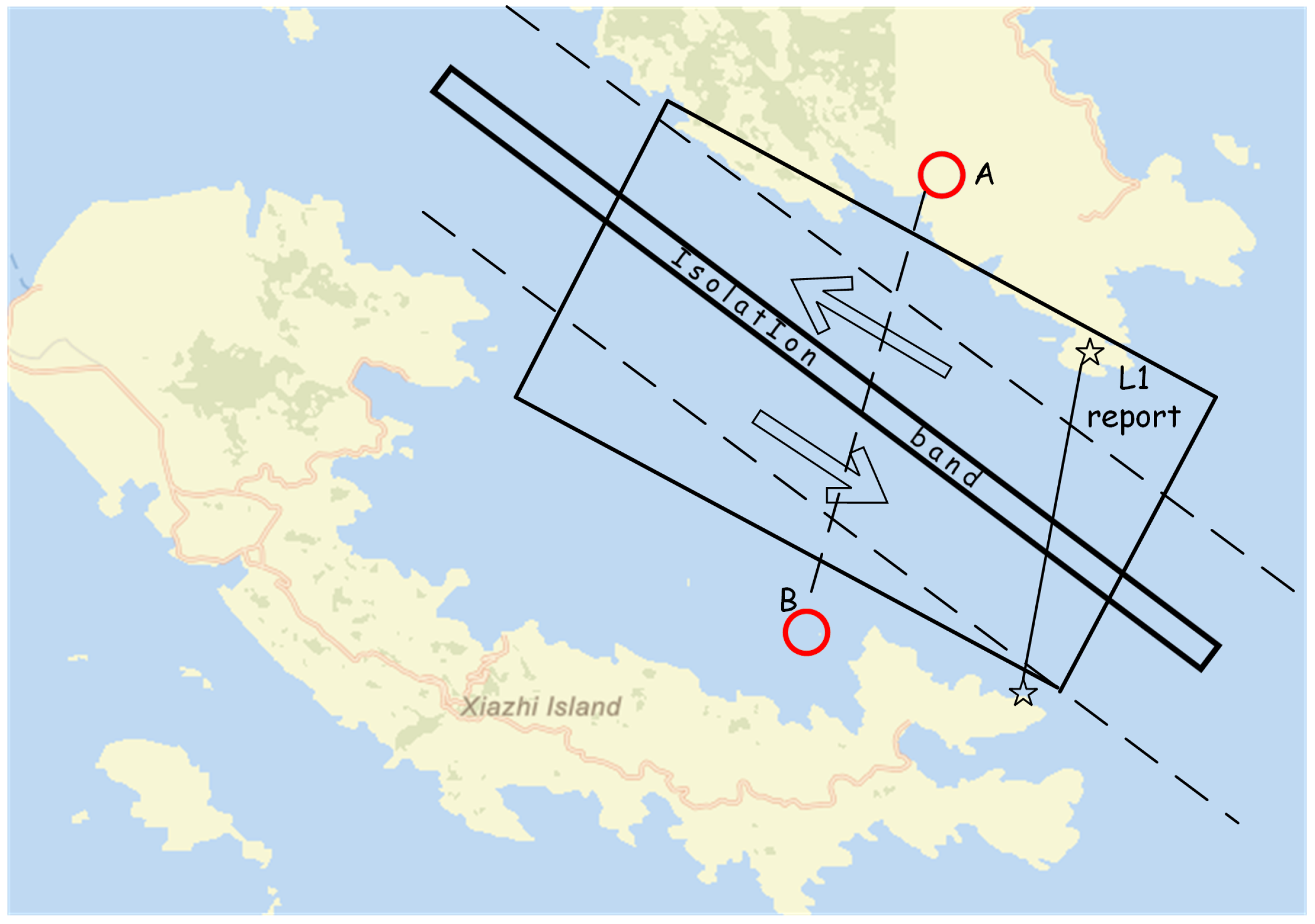
In this paper, the cross-sectional vessel traffic flow every 30 min in Xiazhimen channel, Ningbo-Zhoushan Port was selected. Vessel flow was attained from automatic identification system (AIS) data. AIS contains both static and dynamic information of ships, such as position, speed, rate of turn, etc. In our study, AIS data were provided by ZhouShan Maritime Administration of China. The observation rectangle is shown in Figure 6, with a length of 3.19 nautical miles and width of 1.04 nautical miles. The time period is from 1 March 2020 to 31 March 2020. The observation line AB is near to the L1 Report Line, where ships passing by are required to send AIS data. This guarantees AIS data of high precision. All AIS raw data we need include the ship’s Maritime Mobile Service Identity (MMSI), latitude, longitude, speed, length, type, and heading.

Table 1. AIS raw data description.

Parameters	Description
Observation Point A	(122°17${}^{\prime }$41.07${}^{″}$ E, 29°47${}^{\prime }$12.64${}^{″}$ N)
Observation Point B	(122°16${}^{\prime }$49.31${}^{″}$ E, 29°45${}^{\prime }$05.96${}^{″}$ N)
Time Span	1 March 2020–31 March 2020
Attributes	MMSI, type, speed, length, longitude, latitude, heading
Records	28,369

lists the detailed information of the raw data.

From previous research, traffic flow is related to the local traffic, and international maritime transport is less affected by weather [36]. For this reason, some statistical analyses are made based on this dataset. The results show that domestic ships account for 68% of the records (19,309 in total) and small ships (length less than 50 m) for 80% of the records (22,716), which means the dataset is representative.

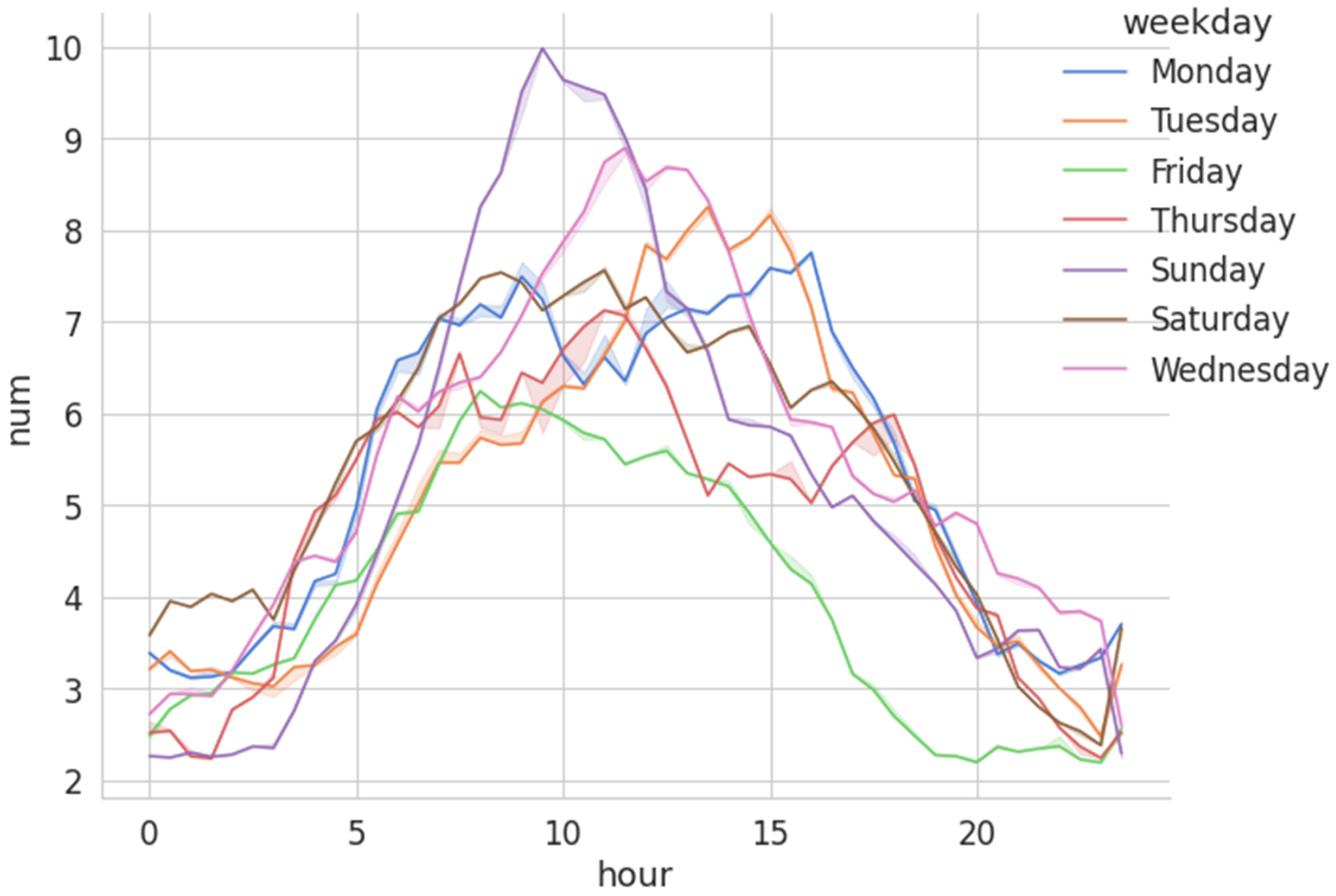
After data cleaning (dropping abnormal records), reliable AIS records were obtained. Set the points $A(ax,ay)$, $B(bx,by)$, and ship position $C(cx,cy)$. Let $S=(ax-cx)(by-cy)-(ay-cy)(bx-cx)$. If $S<0$, we consider C to be on the left of line AB, else it is on the right. A change of the sign of S indicates the very ship passing by. We sampled every three minutes to record the exact number of ships passing the line. The 30-min interval flow data are acquired by adding the values of 10 points together. Then, we denoise the sequence by wavelet to get the smooth flow data [42]. AIS data are then transformed into the flow data. Figure 7 presents the hourly vessel flow in a week at the 95% confidence level.

The weather data, including precipitation and temperature, were accessed from the National Oceanic and Atmospheric Administration (NOAA) website. After processing, there were 1488 sets of data in total. The time span for training is from 1 March 2020 to 25 March 2020, and for testing the span is from 26 March 2020 to 31 March 2020.

Table 2. Dataset description.

Dataset	Xiazhimen Channel
Type	3D time series
Observation Point A	(122°17${}^{\prime }$41.07${}^{″}$ E, 29°47${}^{\prime }$12.64${}^{″}$ N)
Observation Point B	(122°16${}^{\prime }$49.31${}^{″}$ E, 29°45${}^{\prime }$05.96${}^{″}$ N)
Interval	30-min
Time Span	1 March 2020–31 March 2020
Attributes	Flow, precipitation, temperature
Records	1488

shows details of our dataset.

3.2. Details and Evaluation Metrics

In this paper, our P&G model was built on Python libraries Keras and Tensorflow. We chose six advanced models from traditional methods (Prophet), shallow networks (SVR and BPNN), and deep learning networks (LSTM, GRU, and S2S). Six hours of historical data (12 points in total) were fed to the model to make one-point prediction in the 30-min future. All experiments were conducted under the same conditions. We set the initial learning rate uniformly to 0.001, batch size 64, and the optimizer Adam. Four metrics were used to measure the bias between true data and the predicting value.

(1) Mean absolute percentage error:

$$MAPE=\frac{1}{n}\sum _{i=1}^n|\frac{y_i-{\stackrel{\wedge }{y}}_i}{y_i}|,$$

(15)

(2) Mean absolute error:

$$MAE=\frac{1}{n}\sum _{i=1}^n|y_i-{\stackrel{\wedge }{y}}_i|,$$

(16)

(3) Mean square error:

$$MSE=\frac{1}{n}\sum _{i=1}^n{(y_i-{\stackrel{\wedge }{y}}_i)}^2,$$

(17)

(4) Root mean square error:

$$RMSE=\sqrt{\frac{1}{n}\sum _{i=1}^n{(y_i-\stackrel{\wedge }{y_i})}^2}.$$

(18)

3.3. Analysis of Results

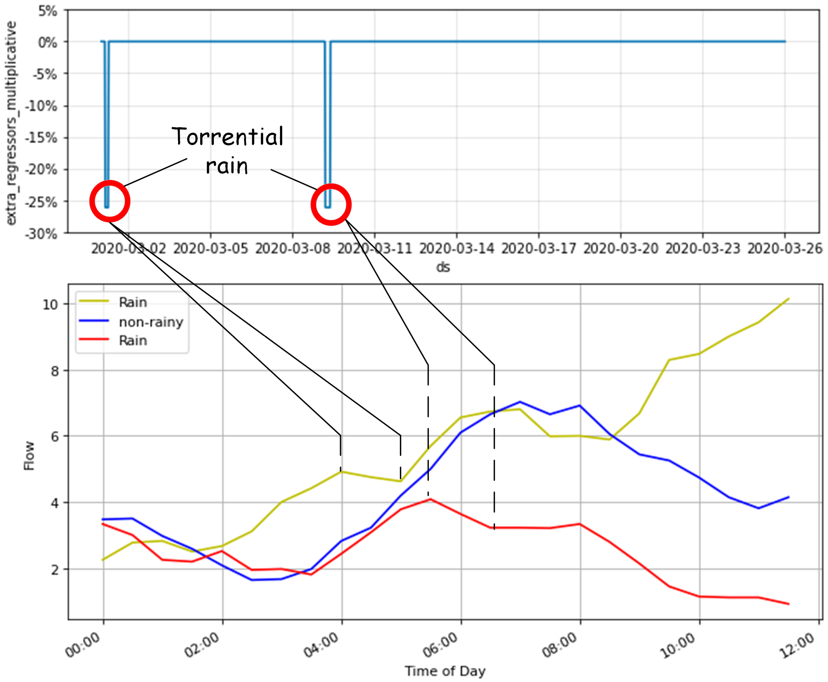
Figure 8 shows components obtained through the Decomposition Layer. From top to bottom are the Trend and Seasonality, including weekly, daily, and hourly terms. Figure 9 draws a connection between Events (precipitation and temperature) and flow in rainy and non-rainy days. Obviously, on occasions of torrential rain (low temperature and high precipitation), traffic flow drops anomalously with an attenuation of 25% to 30%, which demonstrates that our P&G model fits the training set well.

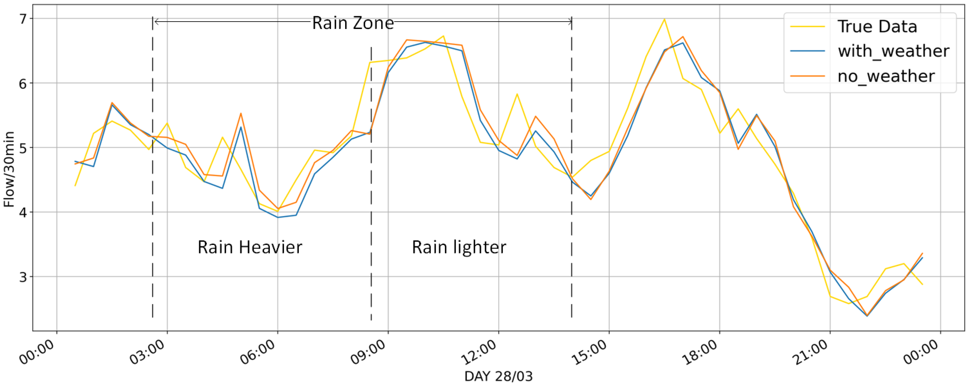
Figure 10 illustrates the performance of the test set, in which the same proposed P&G model with and without weather data are compared. History data records show that it rained from 02:30 to 14:00 on 28 March 2020. In the no-rain zone, the two models differ slightly, but in the rain zone, the proposed model considering weather influence (the line “with_weather”) tends to be lower than the model not considering it (the line “no_weather”), and closer to true data most of the time. The effects are more clear when the rain is heavy.

In Figure 11, comparison results are shown on the test set of the proposed P&G model, Prophet, BPNN, SVR, LSTM, GRU, and S2S. Intuitively, all these models can predict well, but deep learning models (LSTM, GRU, S2S, and P&G) work best.

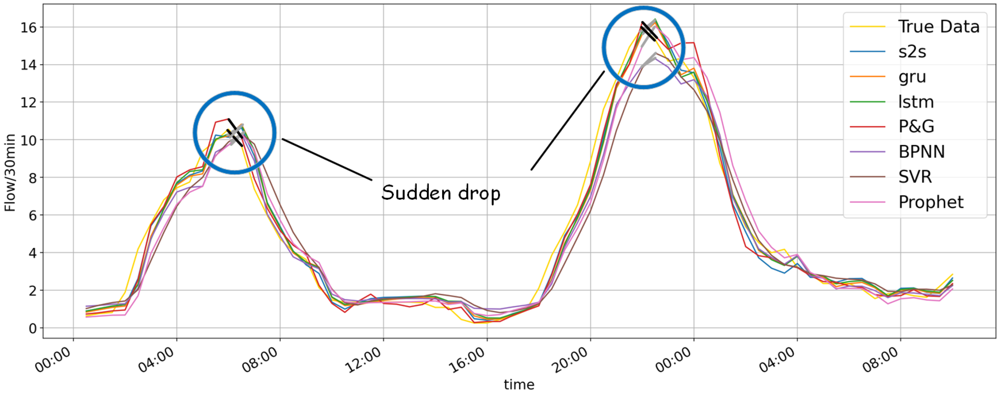
For further comparative analysis, we then examined the tracing ability, as shown in Figure 12. There is a sudden drop when daily flow climbs to the peak. All models except our P&G display lags at the peak. It would be erroneous if we assumed heavy traffic when the flow decreases in reality. However, our P&G model can often capture the sudden drop of the true value one or more steps ahead of other models, thus predicting the sudden change and tracing the real flow simultaneously.

The quantitative indicators are listed in

Table 3. Evaluation metrics.

Models	MAPE	MAE	MSE	RMSE
Prophet	14.457%	0.546	0.537	0.732
BPNN	19.511%	0.553	0.510	0.714
SVR	22.712%	0.605	0.674	0.821
LSTM	13.978%	0.470	0.353	0.594
GRU	13.755%	0.468	0.347	0.588
s2s(GRU-GRU)	12.833%	0.463	0.336	0.580
P&G	9.573%	0.411	0.282	0.531

. Errors of Prophet, BPNN, SVR, LSTM, GRU, S2S, and our proposed model are illustrated for the single-step prediction task. A smaller value reveals a closer prediction to true data. Prophet has almost the same MAE as BPNN but gets 5% less in MAPE, which indicates that Prophet has a stronger long-term memory: predicting small values with smaller errors. GRU, LSTM, and S2S outperformed Prophet slightly (MAPE less than 2%) but get a decrease in MAE of nearly 20%. The proposed model combines merits of both Prophet and deep networks and is superior to other models in all indicators, which means that nonlinear changes and long-term characteristics are actually gained.

4. Conclusions

Short-term vessel traffic flow prediction is vital for areas where incidents can happen due to traffic density. For a more realistic prediction, influencing factors such as weather and tides should be considered. However, limited research has been conducted on the impact how weather affects vessel traffic. To achieve short-term ship traffic flow prediction with higher precision, this paper proposes a multimodal learning model combining weather conditions. First, the basic framework of Sequence2Sequence can better express short-term nonlinear correlation features. Second, by adopting Prophet, long-term features of the sequence are also learned. Finally, weather conditions such as precipitation and temperature are taken as regressors to make the model robust.

A number of experiments are conducted in this paper to test the proposed model compared to other advanced models. The results show that this model outperforms all other models, with an error of 9.573%. Moreover, this model shows a great ability in tracing real-time traffic at the peak of daily flow. In cases of heavy rain, our model is more resilient, providing reliable decision-making and management basis for ships and institutions.

Although this data-driven model performs well in most conditions, it processes related features roughly. Weather data (precipitation and temperature) are treated as dipolar: over a certain threshold (marked as 1) or not (marked as 0). In this way, a gradual change in weather is neglected, which may result in exaggerated predicting results under conditions such as light rain. For future research, we may give attention to how deep weather conditions can affect traffic flow with quantization measures. From the maritime safety point of view, we may consider how local traffic affects the general vessel traffic to get better prediction results.

References

1. Baldauf, M.; Fischer, S.; Kitada, M.; Mehdi, R.; Al-Quhali, M.; Fiorini, M. Merging conventionally navigating ships and MASS-merging VTS, FOC and SCC? TransNav Int. J. Mar. Navig. Saf. Sea Transp. 2019, 13, 495–501. [Google Scholar] [CrossRef]
2. Praetorius, G. Vessel Traffic Service (VTS): A Maritime Information Service or Traffic Control System?: Understanding Everyday Performance and Resilience in a Socio-Technical System under Change. Ph.D. Thesis, Chalmers Tekniska Högskola, Gothenburg, Sweden, 2014. [Google Scholar]
3. Relling, T.; Praetorius, G.; Hareide, O.S. A socio-technical perspective on the future Vessel Traffic Services. Necesse 2019, 4, 112–129. [Google Scholar]
4. Contreras, J.; Espinola, R.; Nogales, F.J.; Conejo, A.J. ARIMA models to predict next-day electricity prices. IEEE Trans. Power Syst. 2003, 18, 1014–1020. [Google Scholar] [CrossRef]
5. Kumar, S.V.; Vanajakshi, L. Short-term traffic flow prediction using seasonal ARIMA model with limited input data. Eur. Transp. Res. Rev. 2015, 7, 1–9. [Google Scholar] [CrossRef] [Green Version]
6. Khodarahmi, M.; Maihami, V. A Review on Kalman Filter Models. Arch. Comput. Methods Eng. 2022, 2022, 1–21. [Google Scholar] [CrossRef]
7. Abidin, A.F.; Kolberg, M.; Hussain, A. Integrating Twitter traffic information with Kalman filter models for public transportation vehicle arrival time prediction. In Big-Data Analytics and Cloud Computing; Springer: Berlin/Heidelberg, Germany, 2015; pp. 67–82. [Google Scholar] [CrossRef]
8. Feng, X.; Ling, X.; Zheng, H.; Chen, Z.; Xu, Y. Adaptive multi-kernel SVM with spatial–temporal correlation for short-term traffic flow prediction. IEEE Trans. Intell. Transp. Syst. 2018, 20, 2001–2013. [Google Scholar] [CrossRef]
9. Li, Y.; Huang, C.; Jiang, J. Research of bus arrival prediction model based on GPS and SVM. In Proceedings of the 2018 Chinese Control and Decision Conference (CCDC), Shenyang, China, 9–11 June 2018; pp. 575–579. [Google Scholar] [CrossRef]
10. Luo, X.; Li, D.; Zhang, S. Traffic flow prediction during the holidays based on DFT and SVR. J. Sens. 2019, 2019, 6461450. [Google Scholar] [CrossRef] [Green Version]
11. Pan, X.; Zhou, W.; Lu, Y.; Sun, N. Prediction of network traffic of smart cities based on DE-BP neural network. IEEE Access 2019, 7, 55807–55816. [Google Scholar] [CrossRef]
12. Ren, C.; An, N.; Wang, J.; Li, L.; Hu, B.; Shang, D. Optimal parameters selection for BP neural network based on particle swarm optimization: A case study of wind speed forecasting. Knowl.-Based Syst. 2014, 56, 226–239. [Google Scholar] [CrossRef]
13. Li, H. Research on prediction of traffic flow based on dynamic fuzzy neural networks. Neural Comput. Appl. 2016, 27, 1969–1980. [Google Scholar] [CrossRef]
14. Cecati, C.; Kolbusz, J.; Różycki, P.; Siano, P.; Wilamowski, B.M. A novel RBF training algorithm for short-term electric load forecasting and comparative studies. IEEE Trans. Ind. Electron. 2015, 62, 6519–6529. [Google Scholar] [CrossRef]
15. Krizhevsky, A.; Sutskever, I.; Hinton, G.E. Imagenet classification with deep convolutional neural networks. Commun. ACM 2017, 60, 84–90. [Google Scholar] [CrossRef] [Green Version]
16. Yu, D.; Liu, Y.; Yu, X. A data grouping CNN algorithm for short-term traffic flow forecasting. In Proceedings of the Asia-Pacific Web Conference, Suzhou, China, 23–25 September 2016; Springer: Berlin/Heidelberg, Germany, 2016; pp. 92–103. [Google Scholar] [CrossRef]
17. Shi, H.; Xu, M.; Li, R. Deep learning for household load forecasting—A novel pooling deep RNN. IEEE Trans. Smart Grid 2017, 9, 5271–5280. [Google Scholar] [CrossRef]
18. Tian, Y.; Pan, L. Predicting short-term traffic flow by long short-term memory recurrent neural network. In Proceedings of the 2015 IEEE International Conference on Smart City/SocialCom/SustainCom (SmartCity), Chengdu, China, 19–21 December 2015; pp. 153–158. [Google Scholar] [CrossRef]
19. Chen, K.; Zhou, Y.; Dai, F. A LSTM-based method for stock returns prediction: A case study of China stock market. In Proceedings of the 2015 IEEE International Conference on Big Data (Big Data), Santa Clara, CA, USA, 29 October 2015–1 November 2015; pp. 2823–2824. [Google Scholar] [CrossRef]
20. Xie, Z.; Liu, Q. LSTM networks for vessel traffic flow prediction in inland waterway. In Proceedings of the 2018 IEEE International Conference on Big Data and Smart Computing (BigComp), Shanghai, China, 15–18 January 2018; pp. 418–425. [Google Scholar] [CrossRef]
21. Fu, R.; Zhang, Z.; Li, L. Using LSTM and GRU neural network methods for traffic flow prediction. In Proceedings of the 2016 31st Youth Academic Annual Conference of Chinese Association of Automation (YAC), Wuhan, China, 11–13 November 2016; pp. 324–328. [Google Scholar] [CrossRef]
22. Shi, X.; Chen, Z.; Wang, H.; Yeung, D.Y.; Wong, W.K.; Woo, W.c. Convolutional LSTM network: A machine learning approach for precipitation nowcasting. Adv. Neural Inf. Process. Syst. 2015, 28. [Google Scholar] [CrossRef]
23. Wang, Y.; Li, L.; Xu, X. A piecewise hybrid of ARIMA and SVMs for short-term traffic flow prediction. In Proceedings of the International Conference on Neural Information Processing, Long Beach, CA, USA, 4–9 December 2017; Springer: Berlin/Heidelberg, Germany, 2017; pp. 493–502. [Google Scholar] [CrossRef]
24. Meng, M.; Shao, C.F.; Wong, Y.D.; Wang, B.B.; Li, H.X. A two-stage short-term traffic flow prediction method based on AVL and AKNN techniques. J. Cent. South Univ. 2015, 22, 779–786. [Google Scholar] [CrossRef]
25. Xie, J.; Choi, Y.K. Hybrid traffic prediction scheme for intelligent transportation systems based on historical and real-time data. Int. J. Distrib. Sens. Netw. 2017, 13, 1550147717745009. [Google Scholar] [CrossRef]
26. Zhang, Z.G.; Yin, J.C.; Wang, N.N.; Hui, Z.G. Vessel traffic flow analysis and prediction by an improved PSO-BP mechanism based on AIS data. Evol. Syst. 2019, 10, 397–407. [Google Scholar] [CrossRef]
27. Hu, Y.L.; Chen, L. A nonlinear hybrid wind speed forecasting model using LSTM network, hysteretic ELM and Differential Evolution algorithm. Energy Convers. Manag. 2018, 173, 123–142. [Google Scholar] [CrossRef]
28. Zhang, J.; Tan, Z.; Wei, Y. An adaptive hybrid model for short term electricity price forecasting. Appl. Energy 2020, 258, 114087. [Google Scholar] [CrossRef]
29. Wang, C.; Zhang, X.; Chen, X.; Li, R.; Li, G. Vessel traffic flow forecasting based on BP neural network and residual analysis. In Proceedings of the 2017 4th International Conference on Information, Cybernetics and Computational Social Systems (ICCSS), Dalian, China, 24–26 July 2017; pp. 350–354. [Google Scholar] [CrossRef]
30. Li, M.W.; Han, D.F.; Wang, W.l. Vessel traffic flow forecasting by RSVR with chaotic cloud simulated annealing genetic algorithm and KPCA. Neurocomputing 2015, 157, 243–255. [Google Scholar] [CrossRef]
31. He, W.; Zhong, C.; Sotelo, M.A.; Chu, X.; Liu, X.; Li, Z. Short-term vessel traffic flow forecasting by using an improved Kalman model. Clust. Comput. 2019, 22, 7907–7916. [Google Scholar] [CrossRef]
32. Smith, B.L.; Williams, B.M.; Oswald, R.K. Comparison of parametric and nonparametric models for traffic flow forecasting. Transp. Res. Part C Emerg. Technol. 2002, 10, 303–321. [Google Scholar] [CrossRef]
33. Pan, Z.; Liang, Y.; Wang, W.; Yu, Y.; Zheng, Y.; Zhang, J. Urban traffic prediction from spatio-temporal data using deep meta learning. In Proceedings of the 25th ACM SIGKDD International Conference on Knowledge Discovery & Data Mining, Anchorage, AK, USA, 4–8 August 2019; pp. 1720–1730. [Google Scholar] [CrossRef]
34. Wang, D.; Meng, Y.; Chen, S.; Xie, C.; Liu, Z. A Hybrid Model for Vessel Traffic Flow Prediction Based on Wavelet and Prophet. J. Mar. Sci. Eng. 2021, 9, 1231. [Google Scholar] [CrossRef]
35. Zhang, D.; Kabuka, M.R. Combining weather condition data to predict traffic flow: A GRU-based deep learning approach. IET Intell. Transp. Syst. 2018, 12, 578–585. [Google Scholar] [CrossRef]
36. Ulusçu, Ö.S.; Özbaş, B.; Altıok, T.; Or, İ. Risk analysis of the vessel traffic in the strait of Istanbul. Risk Anal. Int. J. 2009, 29, 1454–1472. [Google Scholar] [CrossRef]
37. Kitada, M.; Baldauf, M.; Mannov, A.; Svendsen, P.A.; Baumler, R.; Schröder-Hinrichs, J.U.; Dalaklis, D.; Fonseca, T.; Shi, X.; Lagdami, K. Command of vessels in the era of digitalization. In Proceedings of the International Conference on Applied Human Factors and Ergonomics, Orlando, FL, USA, 21–25 July 2018; Springer: Berlin/Heidelberg, Germany, 2018; pp. 339–350. [Google Scholar] [CrossRef]
38. Martínez de Osés, F.X.; Uyà Juncadella, À. Global maritime surveillance and oceanic vessel traffic services: Towards the e-navigation. WMU J. Marit. Aff. 2021, 20, 3–16. [Google Scholar] [CrossRef]
39. Baldauf, M.; Benedict, K.; Krüger, C. Potentials of e-navigation–enhanced support for collision avoidance. TransNav Int. J. Mar. Navig. Saf. Sea Transp. 2014, 8, 613–617. [Google Scholar] [CrossRef] [Green Version]
40. Taylor, S.J.; Letham, B. Forecasting at Scale. Am. Stat. 2018, 72, 37–45. [Google Scholar] [CrossRef]
41. Bracewell, R.N.; Bracewell, R.N. The Fourier Transform and Its Applications; McGraw-Hill: New York, NY, USA, 1986; Volume 31999. [Google Scholar]
42. Srivastava, M.; Anderson, C.L.; Freed, J.H. A New Wavelet Denoising Method for Selecting Decomposition Levels and Noise Thresholds. IEEE Access 2016, 4, 3862–3877. [Google Scholar] [CrossRef]
Figure 1. Diagram of the predicting task. Multimodal inputs including vessel traffic sequence and weather sequence are processed through three layers to attain the predicting vessel value at future time n + τ .
Jmse 11 00039 g001
Figure 2. Flow diagram of the P&G model. Vessel flow and weather data are received as inputs and pass through three layers: Decomposing Layer, Processing Layer, and Joint Prediction Layer to make final predictions.
Jmse 11 00039 g002
Figure 3. Naive RNN structure and a typical GRU.
Jmse 11 00039 g003
Figure 4. GRU-Attention-GRU as S2S structure. The GRUs serve as the encoder and the decoder, and the attention mechanism serves as the variable context vector.
Jmse 11 00039 g004
Figure 5. Mask mechanism to avoid information leakage. The black units are the masked ones.
Jmse 11 00039 g005
Figure 6. Observation zone in Ningbo-Zhoushan Port.
Jmse 11 00039 g006
Figure 7. Hourly vessel traffic flow every week at the 95% confidence level.
Jmse 11 00039 g007
Figure 8. Components Trend and Seasonality (weekly and daily terms).
Jmse 11 00039 g008
Figure 9. Influences of Events (torrential rain) on real traffic flow. On days of heavy rain, the total flow decreases by approximately 25% to 30%.
Jmse 11 00039 g009
Figure 10. Comparison of real observed data, P&G model (with weather data) and P&G model (without weather data) of the test set on 28 March 2020, when there was a heavy rain according to the local history records.
Jmse 11 00039 g010
Figure 11. Comparison of real observed data, P&G model, Prophet, BP, SVR, LSTM, GRU, and S2S during one day (26 March 2020) for the test set. Deep networks appear to be closer to the real value.
Jmse 11 00039 g011
Figure 12. Comparision of tracing ability in P&G, S2S, GRU, LSTM, BP, SVR, and Prophet on 29 March 2020–30 March 2020. Only the proposed model traces the falling tendency at the peak of real flow curve, whereas other methods lag one or two steps.
Jmse 11 00039 g012