

Study of the Performance of Deep Learning Methods Used to Predict Tidal Current Movement

 ,
, 
Abstract
:1. Introduction
2. Methods
- 1.
- To predict and analyze tidal current changes in target seas using a numerical model;
- 2.
- To construct neural networks based on simulation results and measurement data using different deep learning methods;
- 3.
- To calibrate tidal current velocity for non-observed periods using the neural networks above.
2.1. Numerical Model
2.2. Deep Learning Methods
2.2.1. Multilayer Perceptrons
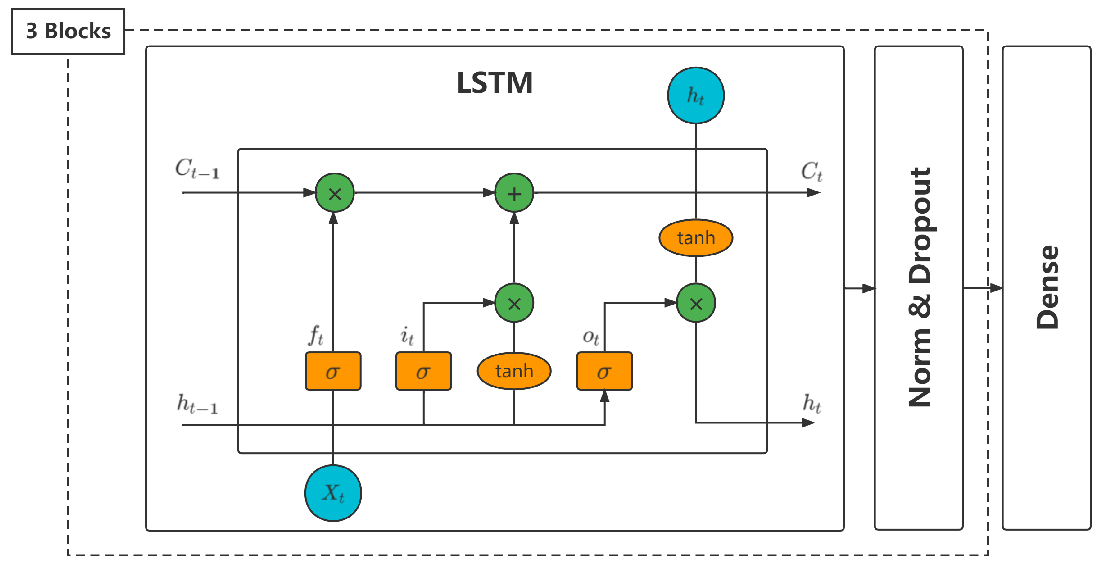
2.2.2. Long Short-Term Memory Network
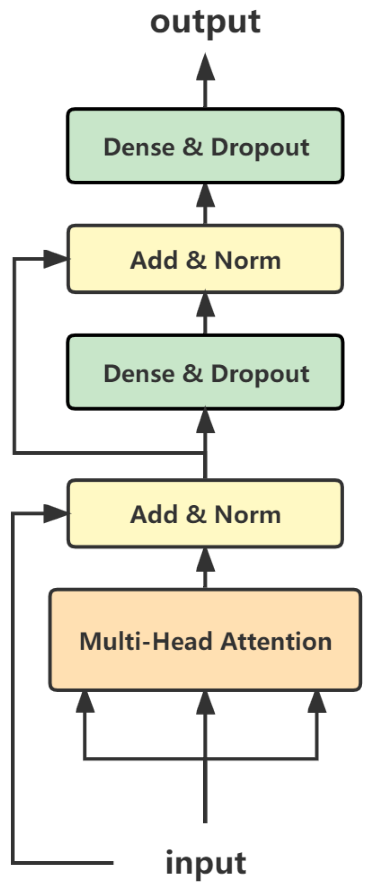
2.2.3. Attention-ResNet Neural Network
3. Experiments
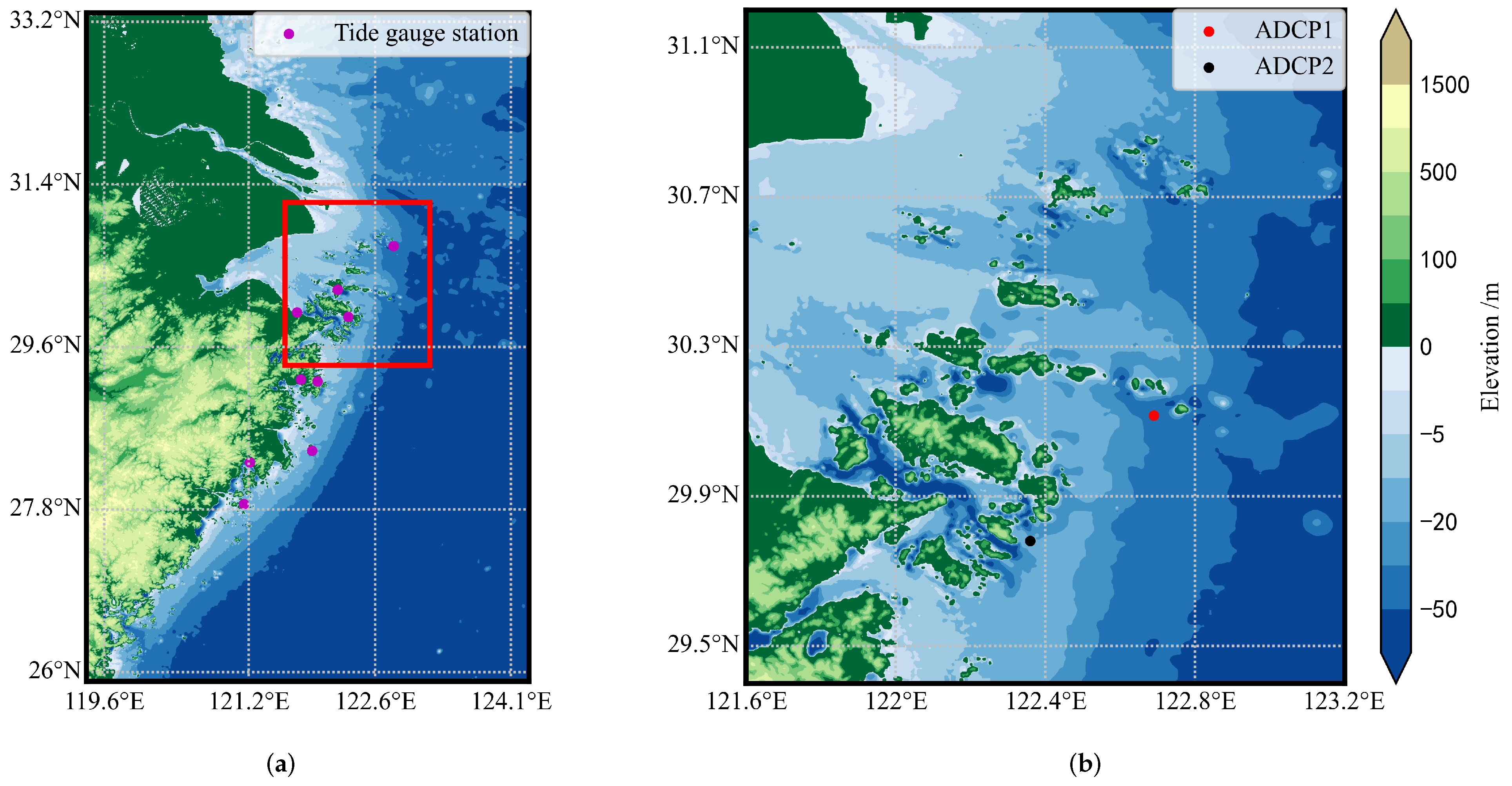
3.1. Numerical Simulation
3.1.1. Simulations
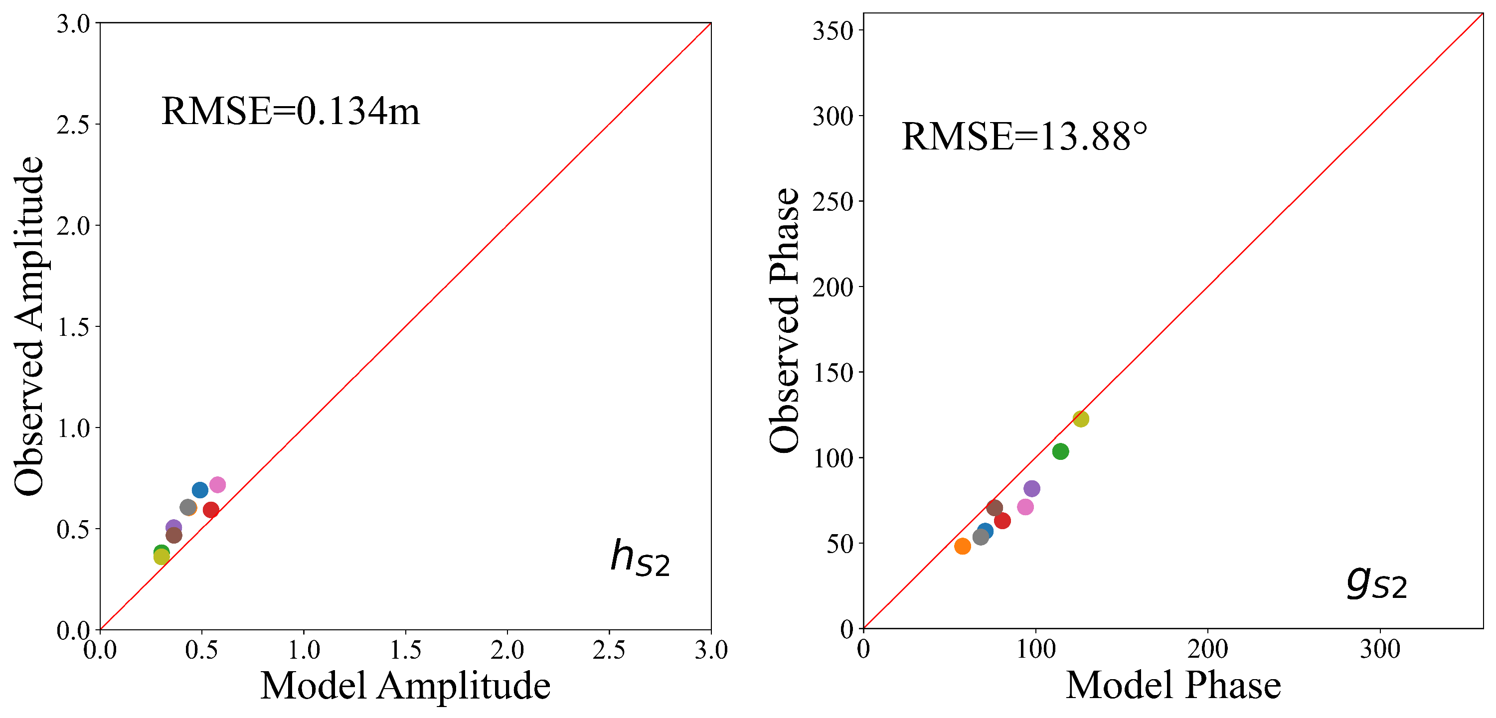
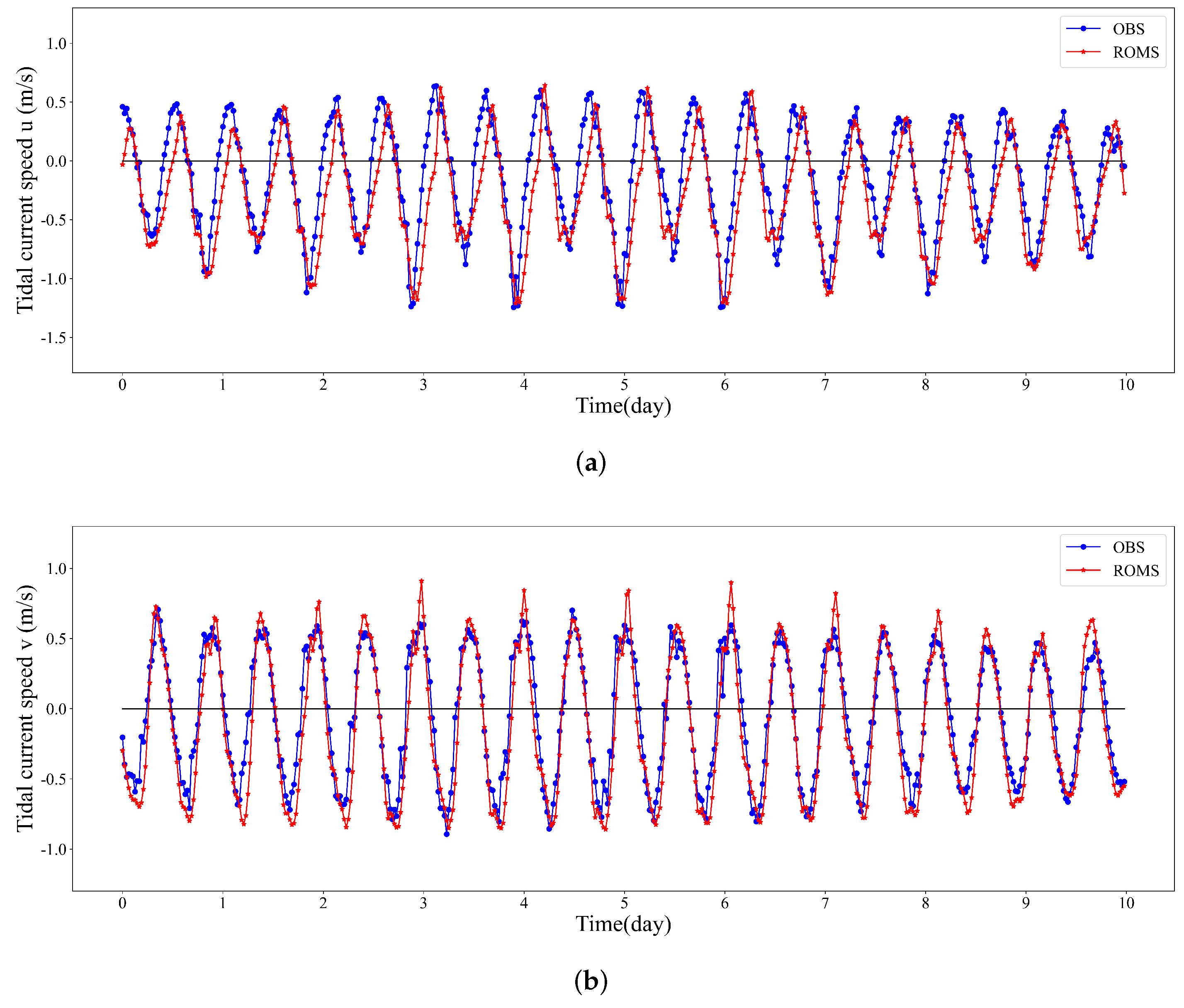
3.1.2. Validation
3.2. Experiment and Results
3.2.1. Datasets
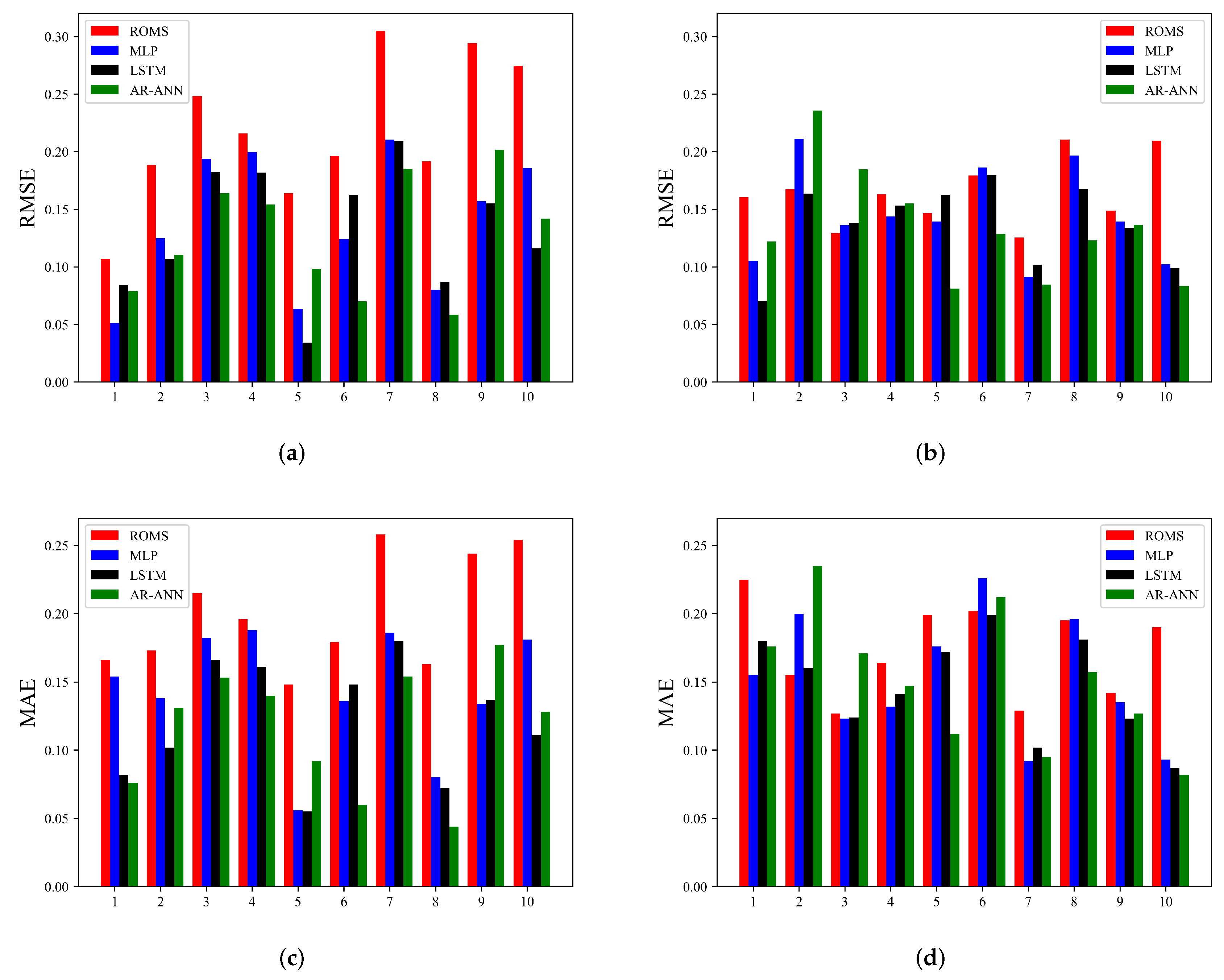
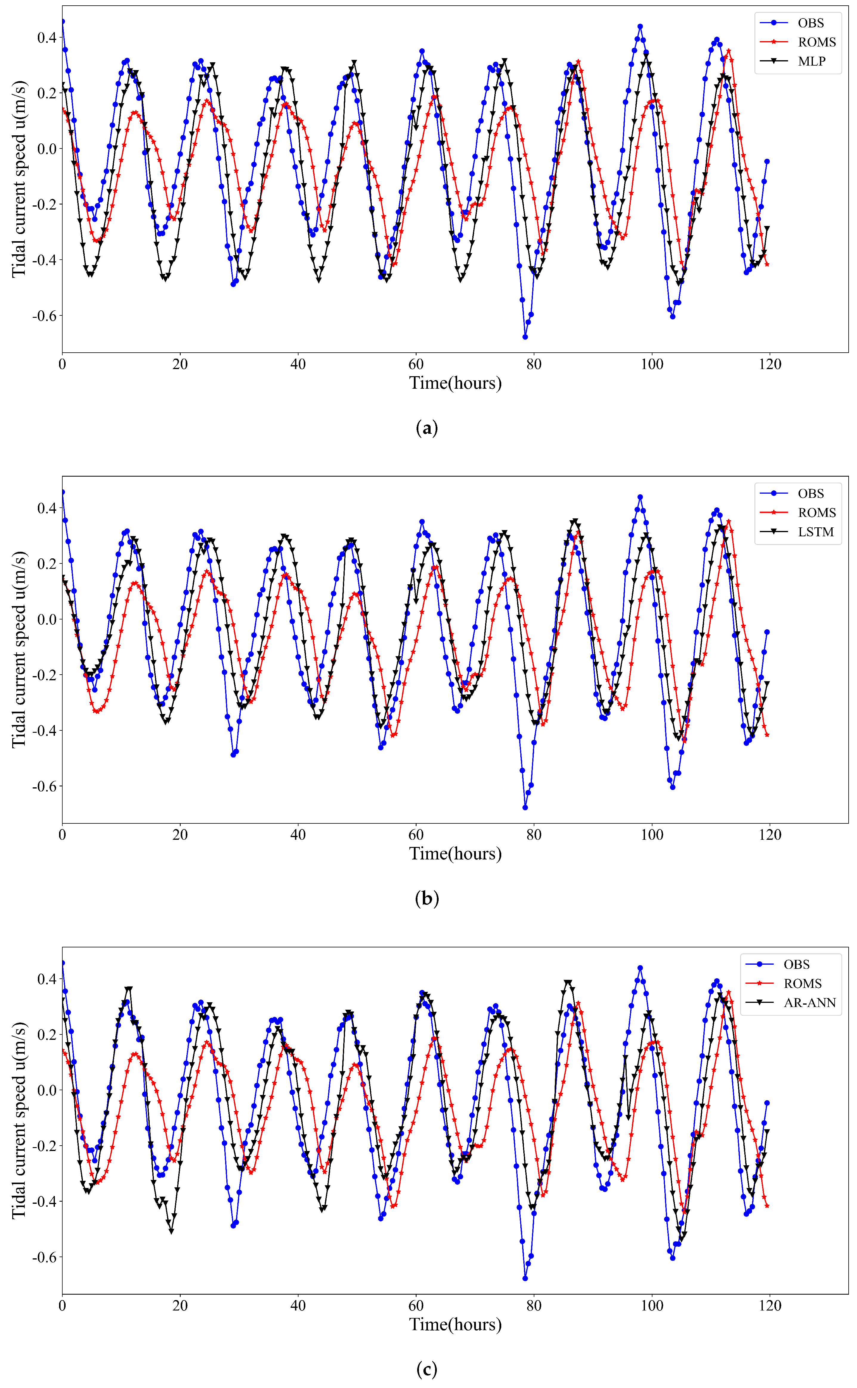
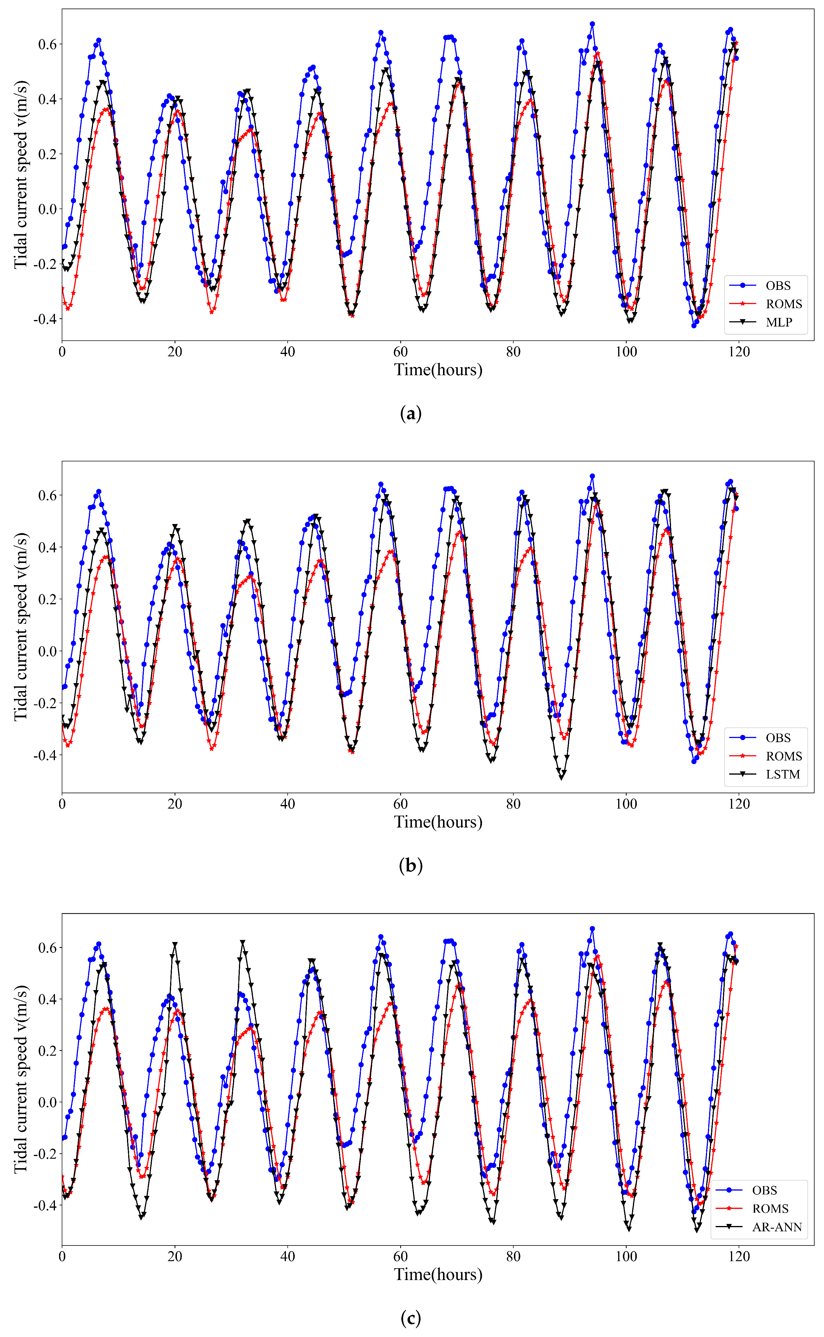
3.2.2. Performance and Model Validation
4. Tidal Current Energy Assessment
5. Conclusions
Author Contributions
Funding
Institutional Review Board Statement
Informed Consent Statement
Data Availability Statement
Conflicts of Interest
Abbreviations
| OBS | Observation |
| MLP | Multilayer perceptron |
| LSTM | Long-short term memory |
| AR-ANN | Attention-ResNet neural network |
| ROMS | Regional Ocean Modeling System |
| ADCP | Acoustic Doppler current profiler |
References
- Li, B.; Chen, W.; Li, J.; Liu, J.; Shi, P. Integrated monitoring and assessments of marine energy for a small uninhabited island. Energy Rep. 2022, 8, 63–72. [Google Scholar] [CrossRef]
- Liu, X.; Chen, Z.; Si, Y.; Qian, P.; Wu, H.; Cui, L.; Zhang, D. A review of tidal current energy resource assessment in China. Renew. Sustain. Energy Rev. 2021, 145, 111012. [Google Scholar] [CrossRef]
- Burić, M.; Grgurić, S.; Mikulčić, H.; Wang, X. A numerical investigation of tidal current energy resource potential in a sea strait. Energy 2021, 234, 121241. [Google Scholar] [CrossRef]
- Uihlein, A.; Magagna, D. Wave and tidal current energy—A review of the current state of research beyond technology. Renew. Sustain. Energy Rev. 2016, 58, 1070–1081. [Google Scholar] [CrossRef]
- Bryden, I.G.; Couch, S.J. How much energy can be extracted from moving water with a free surface: A question of importance in the field of tidal current energy? Renew. Energy 2007, 32, 1961–1966. [Google Scholar] [CrossRef]
- Zhang, J.; Moreau, L.; Machmoum, M.; Guillerm, P.-E. State of the art in tidal current energy extracting technologies. In Proceedings of the 2014 First International Conference on Green Energy ICGE 2014, Sfax, Tunisia, 25–27 March 2014; pp. 1–7. [Google Scholar] [CrossRef]
- Marsh, P.; Penesis, I.; Nader, J.R.; Cossu, R.; Auguste, C.; Osman, P.; Couzi, C. Tidal current resource assessment and study of turbine extraction effects in Banks Strait, Australia. Renew. Energy 2021, 180, 1451–1464. [Google Scholar] [CrossRef]
- Pawlowicz, R.; Beardsley, B.; Lentz, S. Classical tidal harmonic analysis including error estimates in MATLAB using T_TIDE. Comput. Geosci. 2002, 28, 929–937. [Google Scholar] [CrossRef]
- Nachtane, M.; Tarfaoui, M.; Goda, I.; Rouway, M. A review on the technologies, design considerations and numerical models of tidal current turbines. Renew. Energy 2020, 157, 1274–1288. [Google Scholar] [CrossRef]
- Garrett, C.; Cummins, P. Limits to tidal current power. Renew. Energy 2008, 33, 2485–2490. [Google Scholar] [CrossRef]
- Darwin, G.H. Ellipsoidal Harmonic Analysis. Philos. Trans. R. Soc. Lond. Ser. A 1901, 197, 461–557. [Google Scholar]
- Sarkar, D.; Osborne, M.; Adcock, T. A Machine Learning Approach to the Prediction of Tidal Currents. In Proceedings of the 26th International Ocean and Polar Engineering Conference, Rhodes, Greece, 26 June–2 July 2016. [Google Scholar]
- Foreman, M.G.G.; Cherniawsky, J.Y.; Ballantyne, V.A. Versatile Harmonic Tidal Analysis: Improvements and Applications. J. Atmos. Ocean. Technol. 2009, 26, 806–817. [Google Scholar] [CrossRef]
- Niwa, Y.; Hibiya, T. Generation of baroclinic tide energy in a global three-dimensional numerical model with different spatial grid resolutions. Ocean Model. 2014, 80, 59–73. [Google Scholar] [CrossRef]
- Freitas, C. The issue of numerical uncertainty. Appl. Math. Model. 2002, 26, 237–248. [Google Scholar] [CrossRef]
- Yao, J.; Wu, W.; Zhao, Z. Motion and Load Prediction of Floating Platform in South China Sea Using Deep Learning and Prototype Monitoring Information. In Proceedings of the ASME 2019 38th International Conference on Ocean, Offshore and Arctic Engineering, Volume 3: Structures, Safety, and Reliability, Glasgow, UK, 9–14 June 2019; p. V003T02A014. [Google Scholar] [CrossRef]
- Najafzadeh, M.; Oliveto, G. Scour Propagation Rates around Offshore Pipelines Exposed to Currents by Applying Data-Driven Models. Water 2022, 14, 493. [Google Scholar] [CrossRef]
- Najafzadeh, M.; Oliveto, G.; Saberi-Movahed, F. Estimation of Scour Propagation Rates around Pipelines While Considering Simultaneous Effects of Waves and Currents Conditions. Water 2022, 14, 1589. [Google Scholar] [CrossRef]
- Chen, X.; Yu, R.; Ullah, S.; Wu, D.; Li, Z.; Li, Q.; Qi, H.; Liu, J.; Liu, M.; Zhang, Y. A novel loss function of deep learning in wind speed forecasting. Energy 2022, 238, 121808. [Google Scholar] [CrossRef]
- Dimililer, K.; Dindar, H.; Al-Turjman, F. Deep learning, machine learning and internet of things in geophysical engineering applications: An overview. Microprocess. Microsyst. 2021, 80, 103613. [Google Scholar] [CrossRef]
- Sarkar, D.; Osborne, M.A.; Adcock, T.A.A. Prediction of tidal currents using Bayesian machine learning. Ocean Eng. 2018, 158, 221–231. [Google Scholar] [CrossRef]
- Kavousi-Fard, A.; Su, W. A Combined Prognostic Model Based on Machine Learning for Tidal Current Prediction. IEEE Trans. Geosci. Remote Sens. 2017, 55, 3108–3114. [Google Scholar] [CrossRef]
- Zhang, A.; Lin, Y.; Sun, Y.; Yuan, H.; Wang, M.; Liu, G.; Hu, Y. Tidal current prediction based on fractal theory and improved least squares support vector machine. IET Renew. Power Gener. 2022, 16, 389–401. [Google Scholar] [CrossRef]
- Riazi, A. Accurate tide level estimation: A deep learning approach. Ocean Eng. 2020, 198, 107013. [Google Scholar] [CrossRef]
- Yang, C.-H.; Wu, C.-H.; Hsieh, C.-M. Long Short-Term Memory Recurrent Neural Network for Tidal Level Forecasting. IEEE Access 2020, 8, 159389–159401. [Google Scholar] [CrossRef]
- Bayindir, C. Predicting the Ocean Currents using Deep Learning. arXiv 2019, arXiv:1906.08066. [Google Scholar]
- Sarkar, D.; Osborne, M.A.; Adcock, T.A.A. Spatiotemporal prediction of tidal currents using Gaussian processes. J. Geophys. Res. Ocean. 2019, 124, 2697–2715. [Google Scholar] [CrossRef]
- Feng, B.; Qian, P.; Si, Y.; Liu, X.; Yang, H.; Wen, H.; Zhang, D. Comparative Investigations of Tidal Current Velocity Prediction Considering Effect of Multi-Layer Current Velocity. Energies 2020, 13, 6417. [Google Scholar] [CrossRef]
- Aly, H.H.H. Intelligent optimized deep learning hybrid models of neuro wavelet, Fourier Series and Recurrent Kalman Filter for tidal currents constitutions forecasting. Ocean Eng. 2020, 218, 108254. [Google Scholar] [CrossRef]
- Shchepetkin, A.F.; McWilliams, J.C. The regional oceanic modeling system (ROMS): A split-explicit, free-surface, topography-following-coordinate oceanic model. Ocean Model. 2005, 9, 347–404. [Google Scholar] [CrossRef]
- Moore, A.M.; Arango, H.G.; Broquet, G.; Powell, B.S.; Weaver, A.T.; Zavala-Garay, J. The Regional Ocean Modeling System (ROMS) 4-dimensional variational data assimilation systems: Part I–System overview and formulation. Prog. Oceanogr. 2011, 91, 34–49. [Google Scholar] [CrossRef]
- Jung, K.; Cho, Y.K.; Tak, Y.J. Containers and orchestration of numerical ocean model for computational reproducibility and portability in public and private clouds: Application of ROMS 3.6. Simul. Model. Pract. Theory 2021, 109, 102305. [Google Scholar] [CrossRef]
- Bradbury, M.C.; Conley, D.C. Using Artificial Neural Networks for the Estimation of Subsurface Tidal Currents from High-Frequency Radar Surface Current Measurements. Remote Sens. 2021, 13, 3896. [Google Scholar] [CrossRef]
- Guo, H.; Guo, C.; Xu, B.; Xia, Y.; Sun, F. MLP neural network-based regional logistics demand prediction. Neural Comput. Appl. 2021, 33, 3939–3952. [Google Scholar] [CrossRef]
- Zhou, K.; Yu, H.; Zhao, W.X.; Wen, J.-R. Filter-enhanced MLP is All You Need for Sequential Recommendation. In Proceedings of the ACM Web Conference 2022, Lyon, France, 25–29 April 2022; pp. 2388–2399. [Google Scholar] [CrossRef]
- Bai, L.-H.; Xu, H. Accurate estimation of tidal level using bidirectional long short-term memory recurrent neural network. Ocean Eng. 2021, 235, 108765. [Google Scholar] [CrossRef]
- Zhang, Z.; Hou, M.; Zhang, F.; Edwards, C.R. An LSTM based Kalman Filter for Spatio-temporal Ocean Currents Assimilation. In Proceedings of the International Conference on Underwater Networks & Systems, Atlanta, GA, USA, 23–25 October 2019; pp. 1–7. [Google Scholar] [CrossRef]
- Vaswani, A.; Shazeer, N.; Parmar, N.; Uszkoreit, J.; Jones, L.; Gomez, A.N.; Kaiser, Ł.; Polosukhin, I. Attention is all you need. In Proceedings of the Advances in Neural Information Processing Systems, Long Beach, CA, USA, 4–9 December 2017; Volume 30. [Google Scholar]
- Xu, Q.S.; Yang, X.H.; Huang, X. Ensemble Residual Networks for Short Term Load Forecasting. IEEE Access 2020, 8, 64750–64759. [Google Scholar] [CrossRef]


| Parameter | MLP | LSTM | AR-ANN |
|---|---|---|---|
| Input Shape | (None,72) | (72,1) | (None,72) |
| Batch Size | 100 | 100 | 100 |
| LSTM Units | / | 300/200/200 | / |
| Dense Units | 300/200/200 | / | 300/200 |
| Head Numbers | / | / | 6 |
| Dropout Rate | 0.3 | 0.3 | 0.3 |
| Epoch | 100 | 100 | 100 |
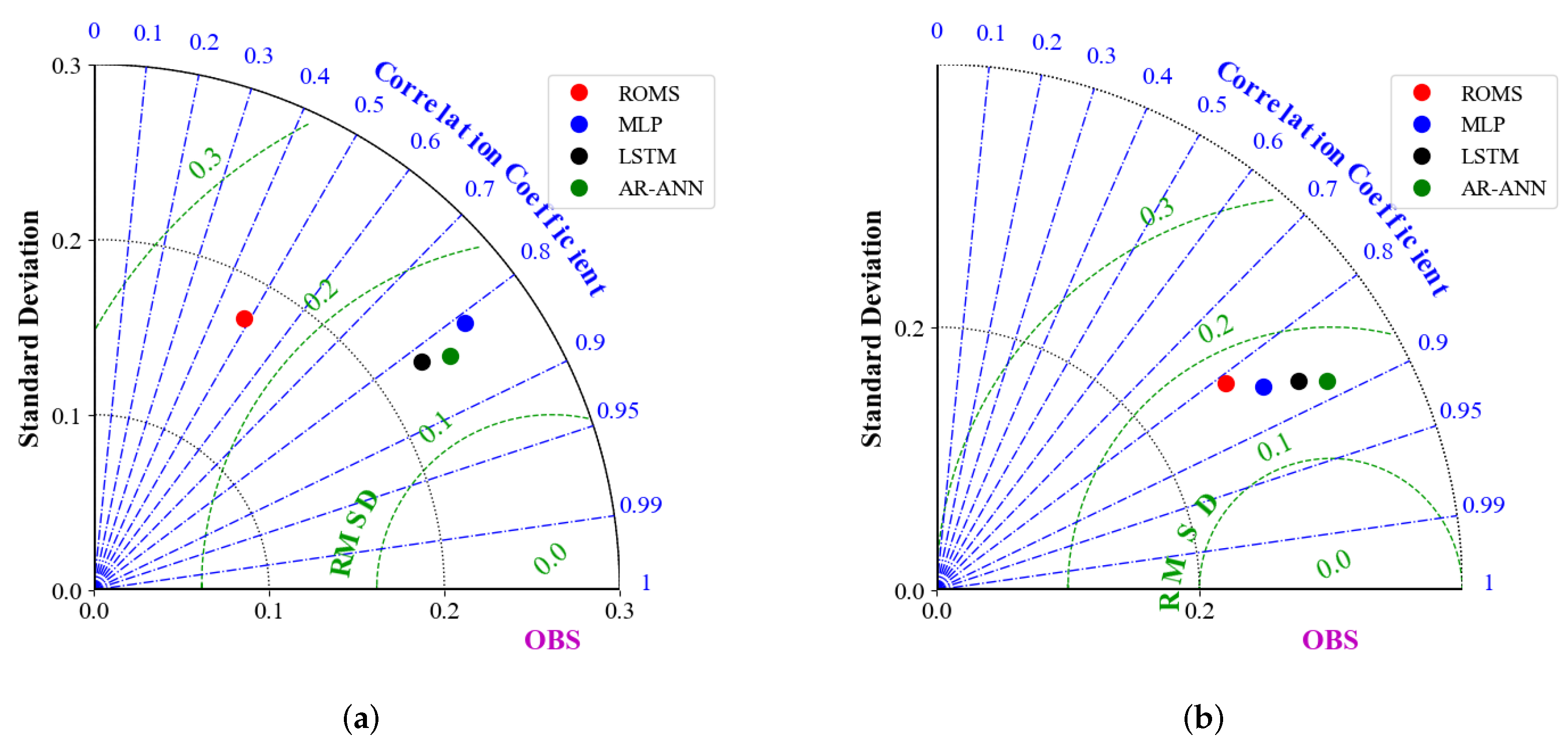
| Variable | Metric | ROMS | MLP | LSTM | AR-ANN |
|---|---|---|---|---|---|
| U | RMSE | 0.234 | 0.160 | 0.150 | 0.146 |
| MAE | 0.200 | 0.143 | 0.121 | 0.113 | |
| R | 0.484 | 0.811 | 0.820 | 0.830 | |
| V | RMSE | 0.176 | 0.163 | 0.161 | 0.153 |
| MAE | 0.173 | 0.153 | 0.147 | 0.152 | |
| R | 0.814 | 0.848 | 0.866 | 0.892 |
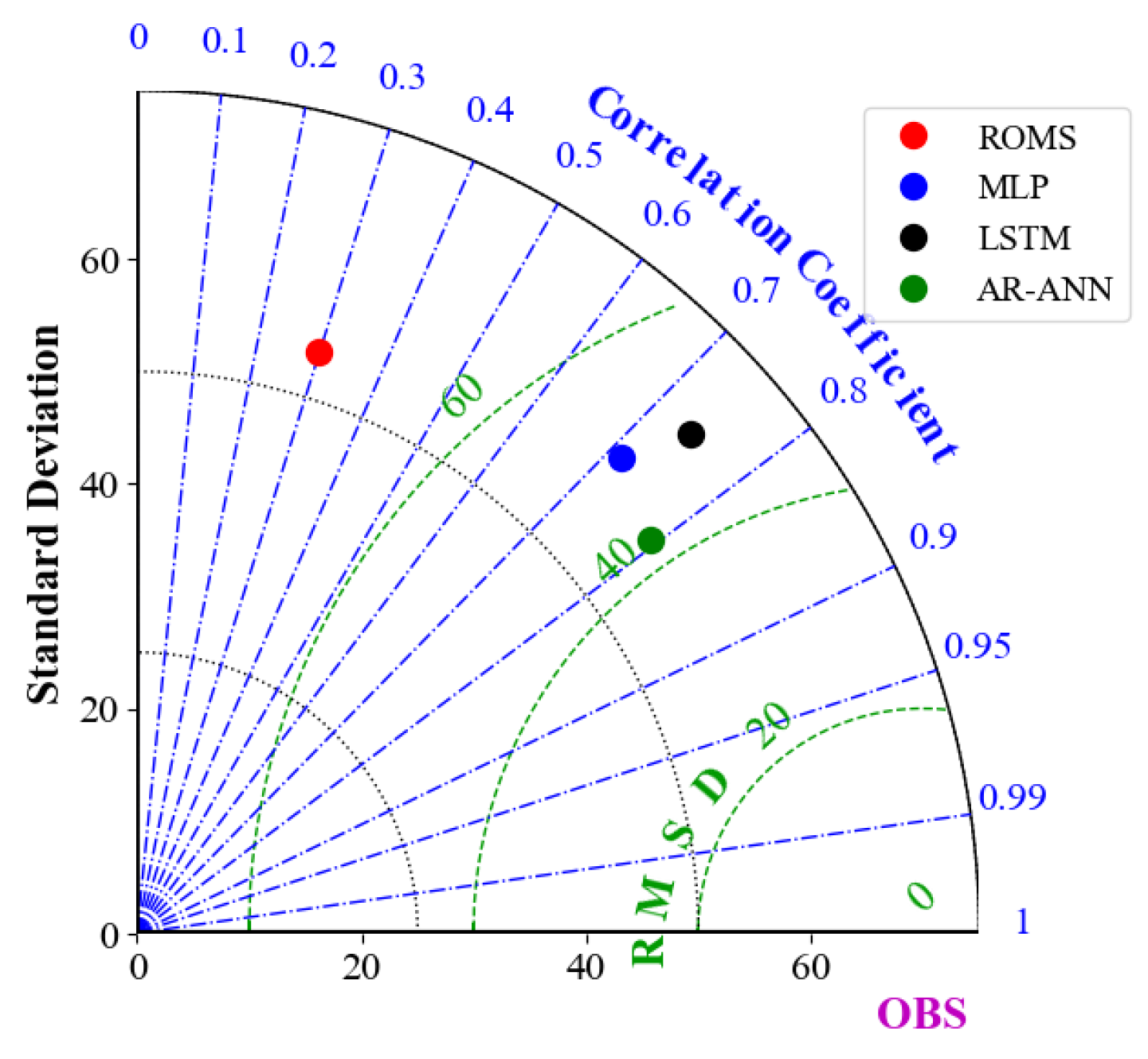
| Metric | ROMS | MLP | LSTM | AR-ANN |
|---|---|---|---|---|
| RMSE | 74.68 | 50.096 | 49.003 | 43.315 |
| MAE | 67.467 | 43.834 | 39.505 | 38.389 |
| R | 0.297 | 0.714 | 0.743 | 0.786 |
Disclaimer/Publisher’s Note: The statements, opinions and data contained in all publications are solely those of the individual author(s) and contributor(s) and not of MDPI and/or the editor(s). MDPI and/or the editor(s) disclaim responsibility for any injury to people or property resulting from any ideas, methods, instructions or products referred to in the content. |
© 2022 by the authors. Licensee MDPI, Basel, Switzerland. This article is an open access article distributed under the terms and conditions of the Creative Commons Attribution (CC BY) license (https://creativecommons.org/licenses/by/4.0/).
Share and Cite
Zhang, K.; Wang, X.; Wu, H.; Zhang, X.; Fang, Y.; Zhang, L.; Wang, H. Study of the Performance of Deep Learning Methods Used to Predict Tidal Current Movement. J. Mar. Sci. Eng. 2023, 11, 26. https://doi.org/10.3390/jmse11010026
Zhang K, Wang X, Wu H, Zhang X, Fang Y, Zhang L, Wang H. Study of the Performance of Deep Learning Methods Used to Predict Tidal Current Movement. Journal of Marine Science and Engineering. 2023; 11(1):26. https://doi.org/10.3390/jmse11010026
Chicago/Turabian StyleZhang, Kai, Xiaoyong Wang, He Wu, Xuefeng Zhang, Yizhou Fang, Lianxin Zhang, and Haifeng Wang. 2023. "Study of the Performance of Deep Learning Methods Used to Predict Tidal Current Movement" Journal of Marine Science and Engineering 11, no. 1: 26. https://doi.org/10.3390/jmse11010026
APA StyleZhang, K., Wang, X., Wu, H., Zhang, X., Fang, Y., Zhang, L., & Wang, H. (2023). Study of the Performance of Deep Learning Methods Used to Predict Tidal Current Movement. Journal of Marine Science and Engineering, 11(1), 26. https://doi.org/10.3390/jmse11010026