

Numerical Evaluation of the Wave-Making Resistance of a Zero-Emission Fast Passenger Ferry Operating in Shallow Water by Using the Double-Body Approach


Abstract
1. Introduction
2. Mathematical Models
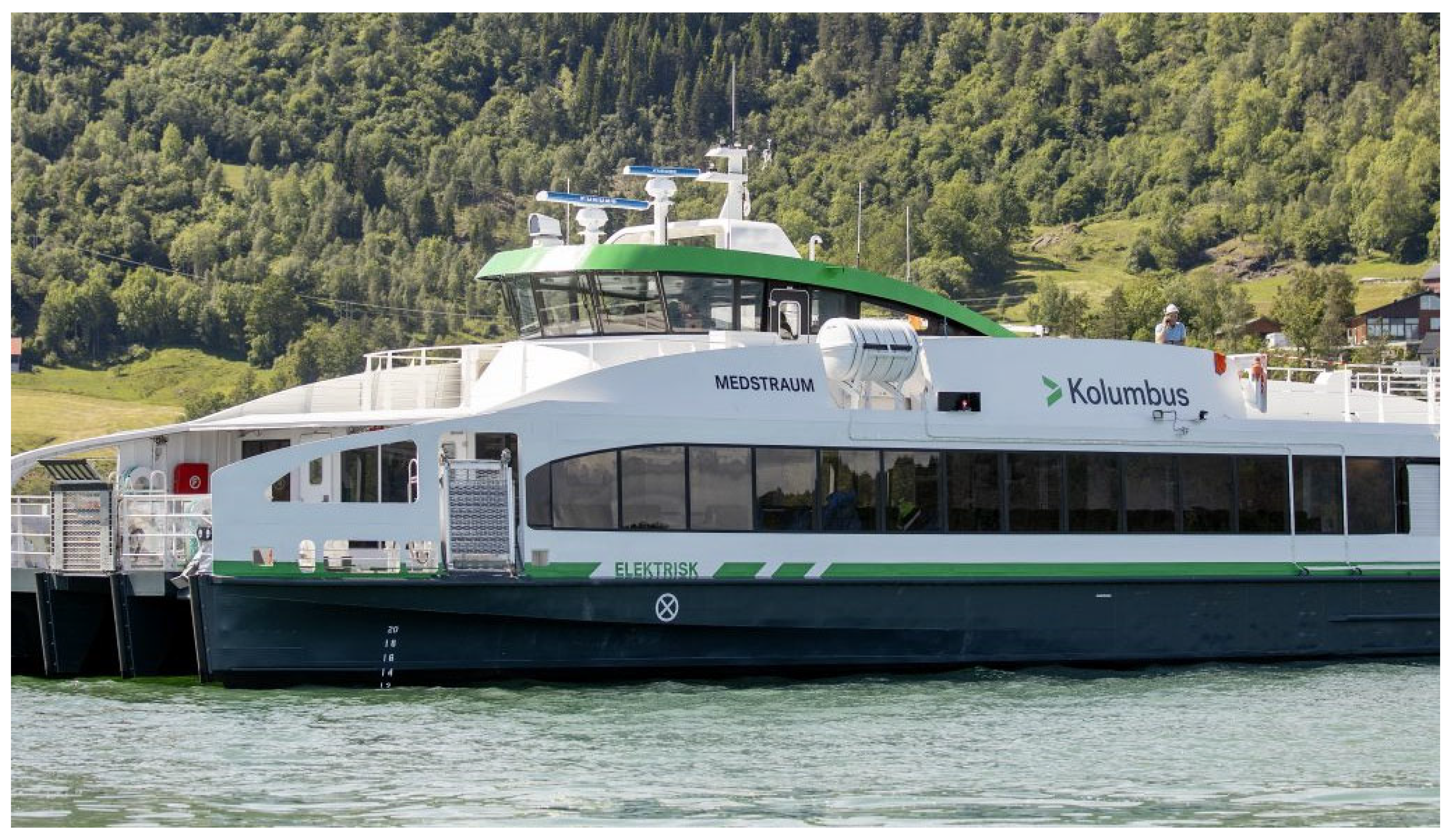
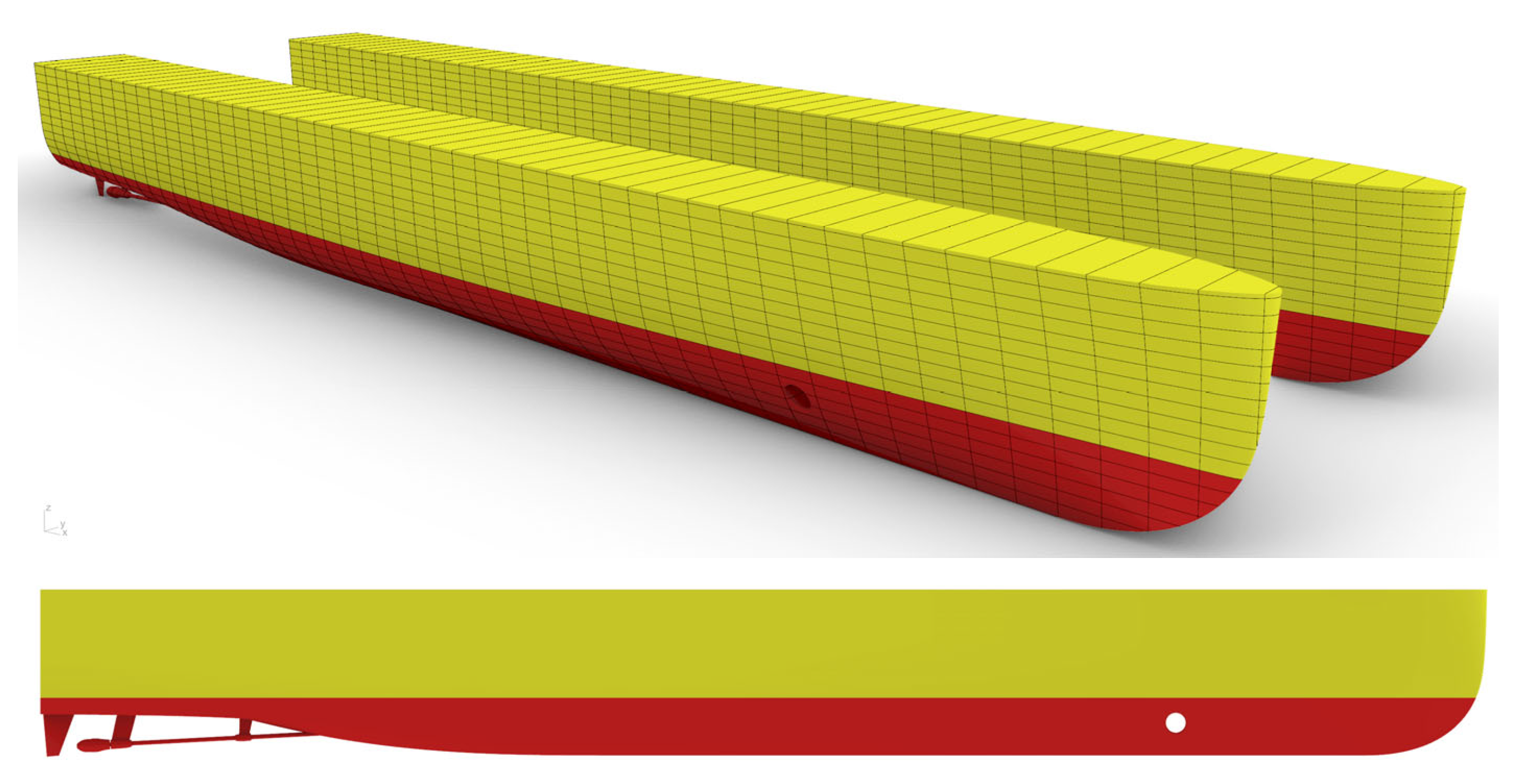
2.1. Geometric Properties of the Catamaran Hull
2.2. Computational Method
2.2.1. Governing Equations
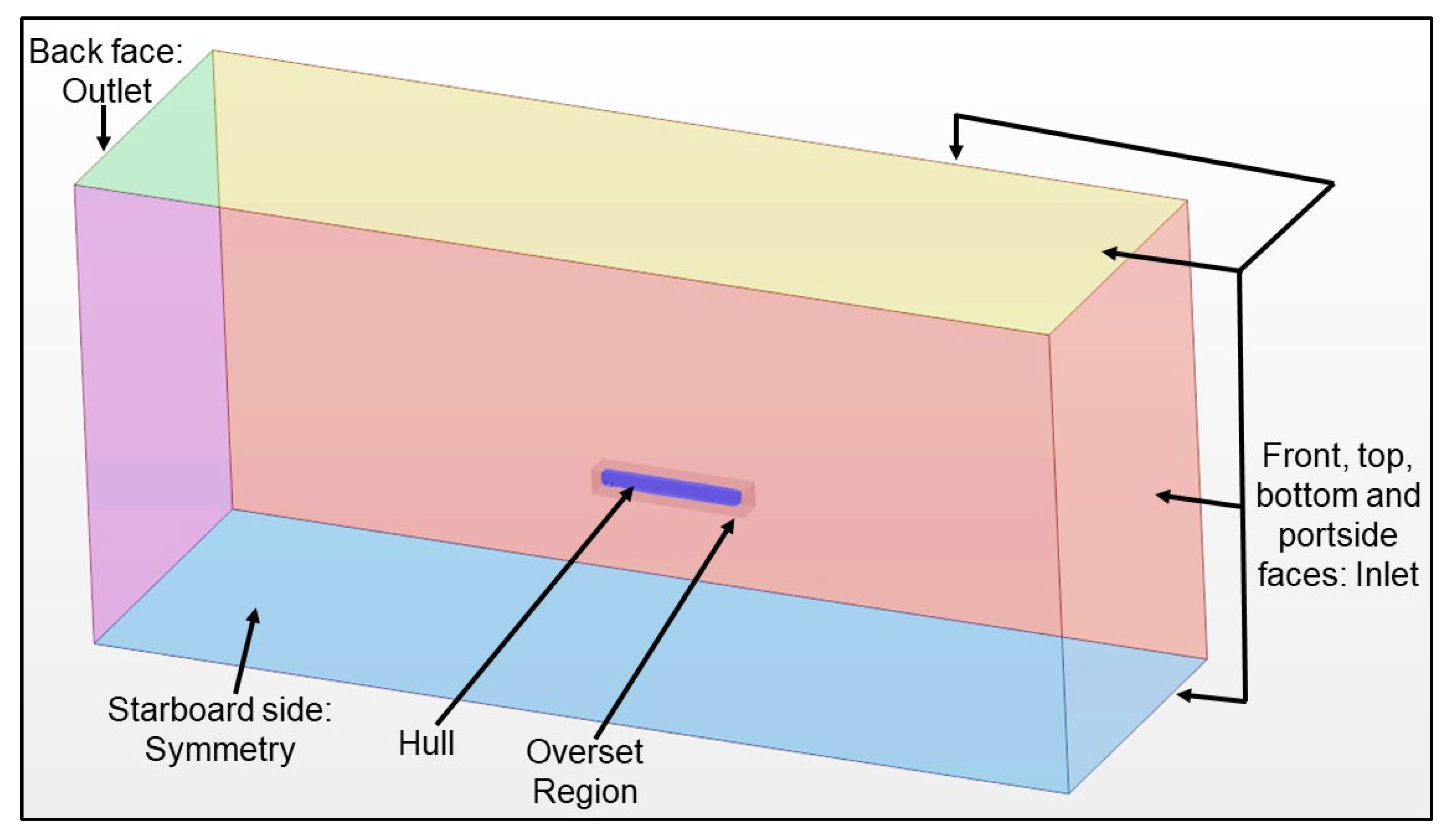
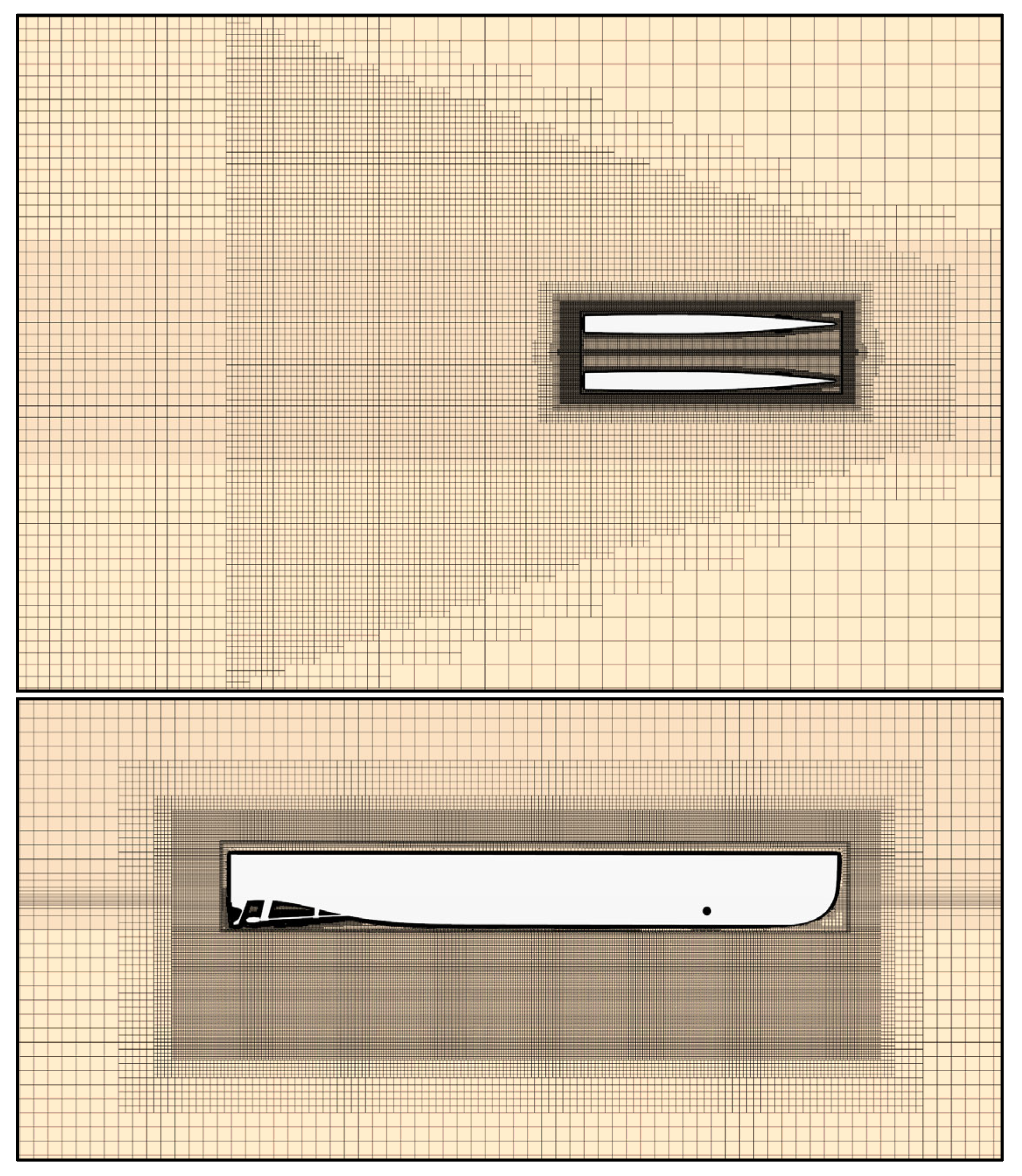
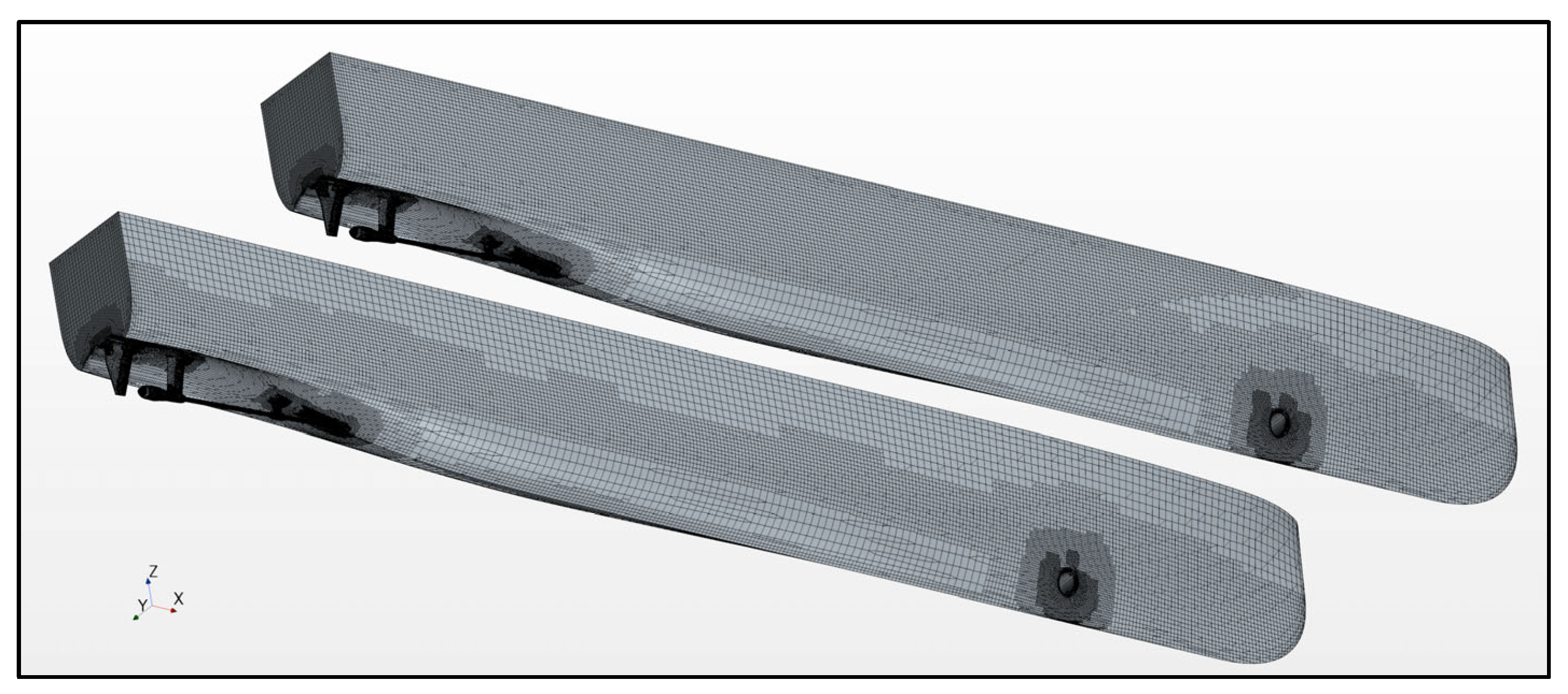
2.2.2. Computational Domain Boundaries and Grid Resolution
2.2.3. Form Factor Prediction Method
2.3. Presentation of Data
3. Results and Discussion
3.1. Verification and Validation Study
3.1.1. Verification
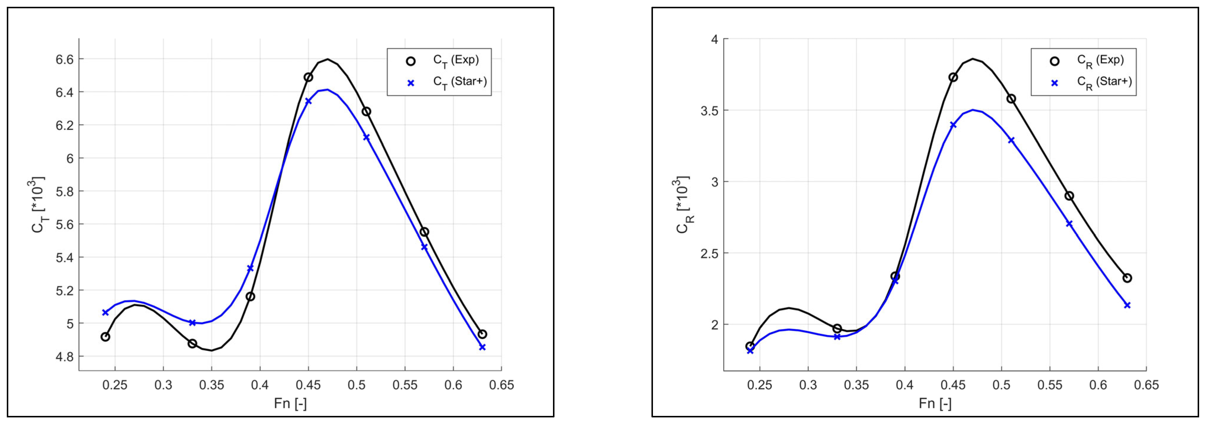
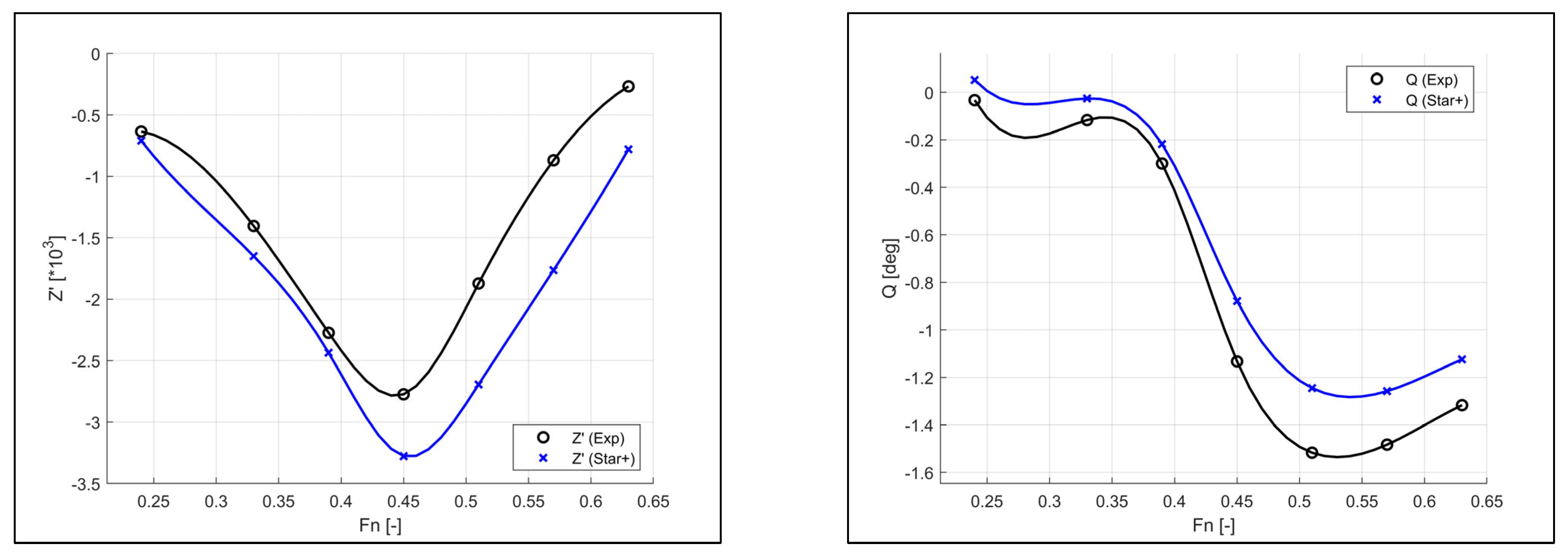
3.1.2. Validation
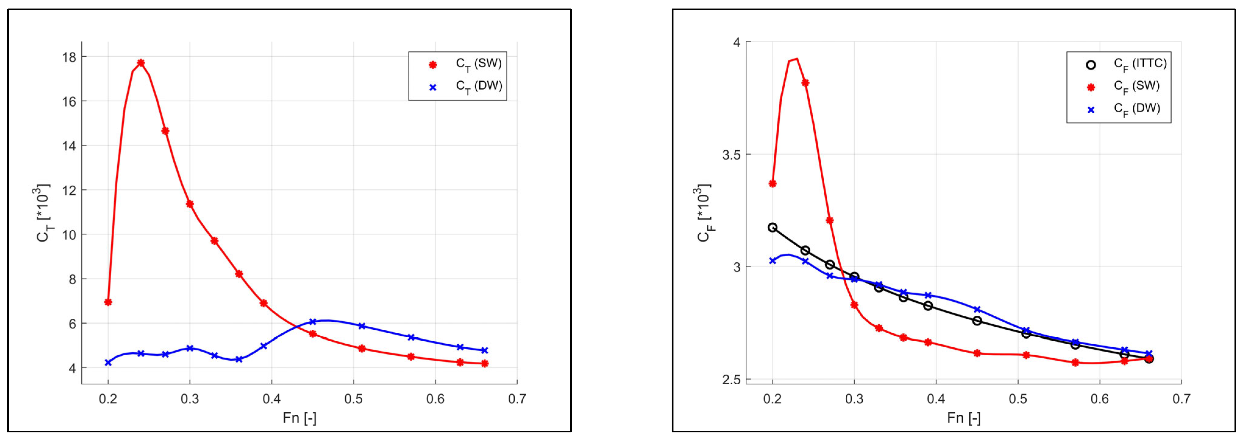
3.2. Deep and Shallow Water Resistance Analysis Results
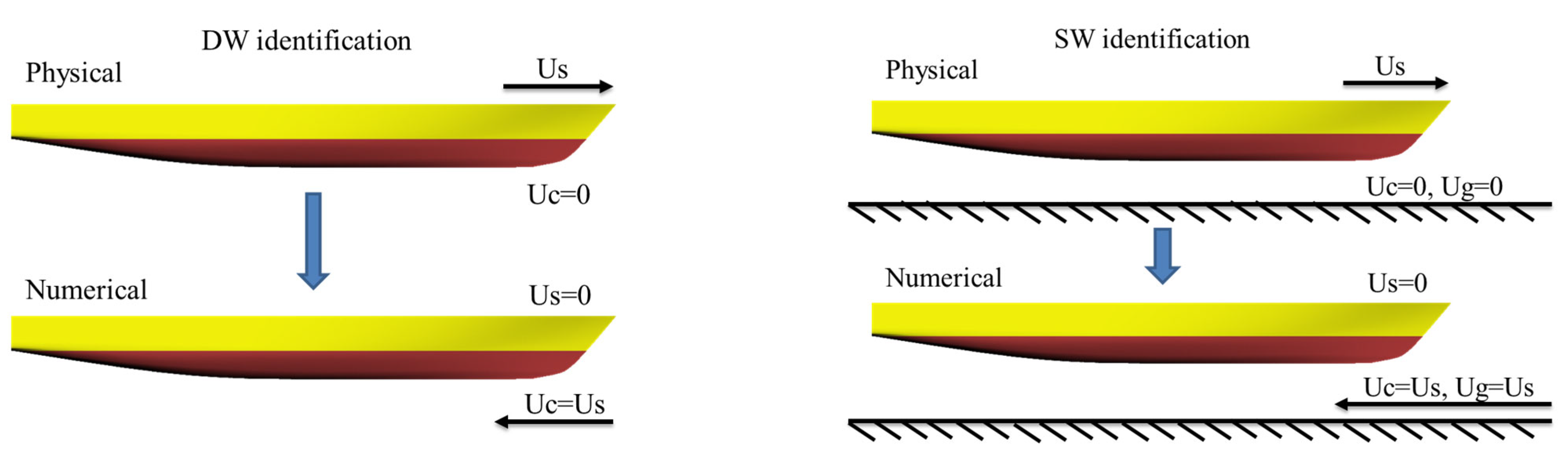
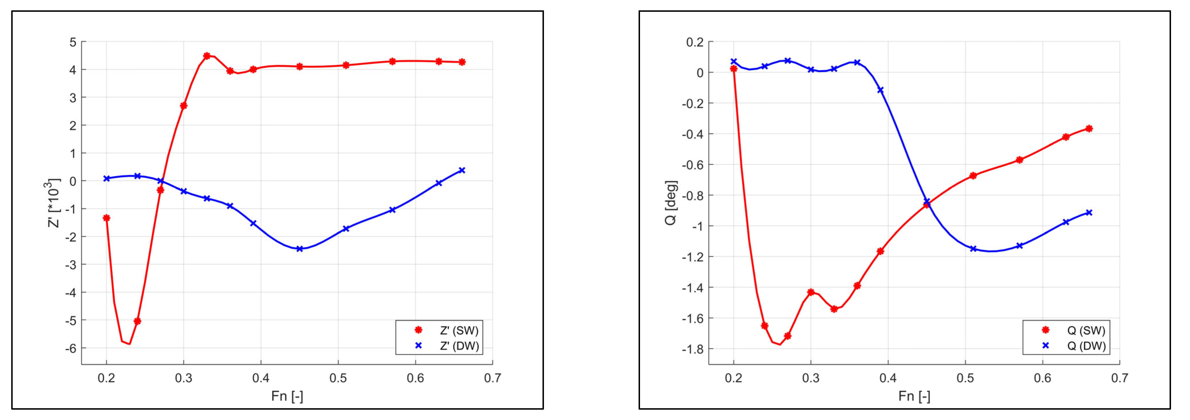
3.3. Double-Body Analysis Results
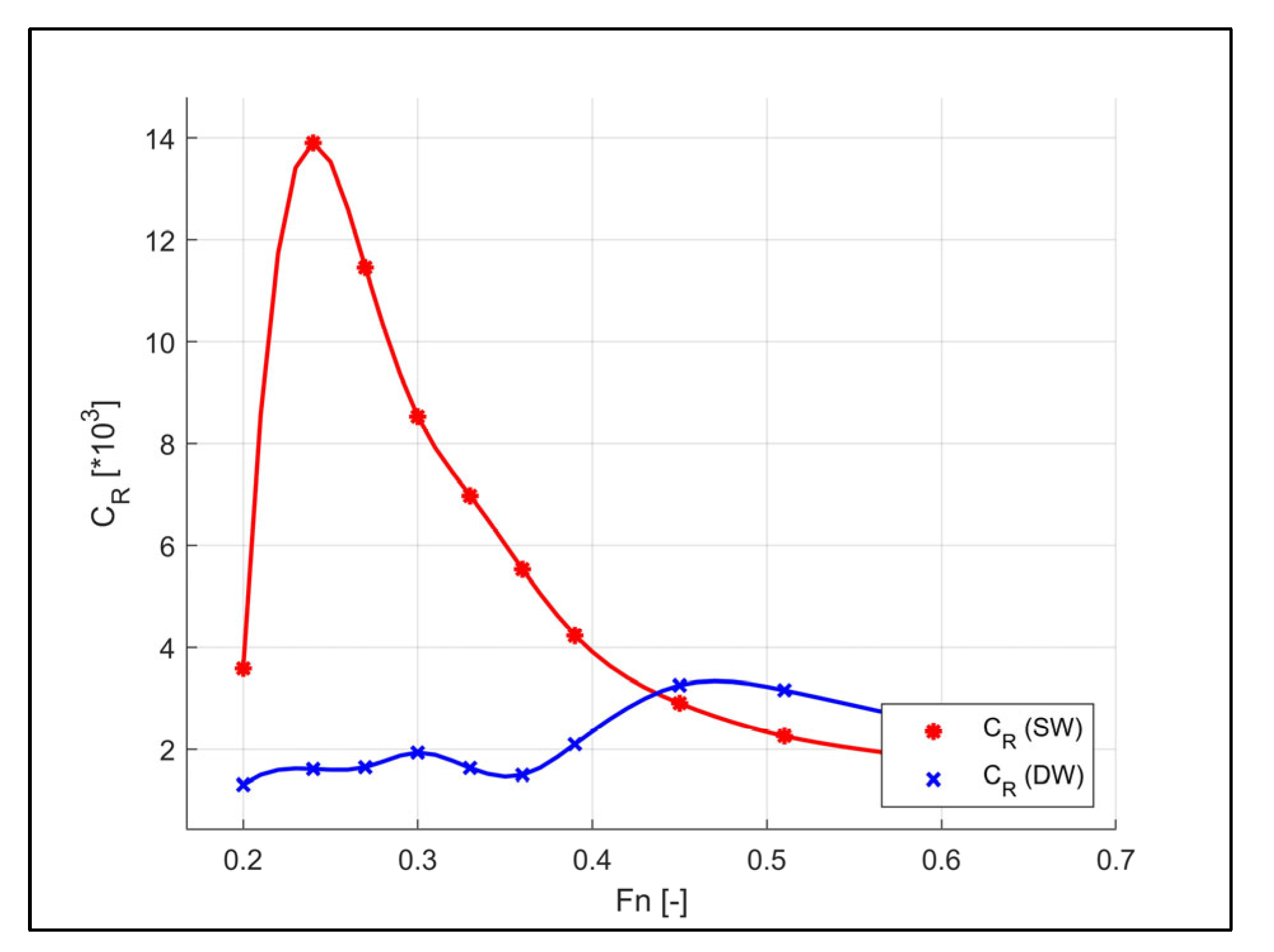
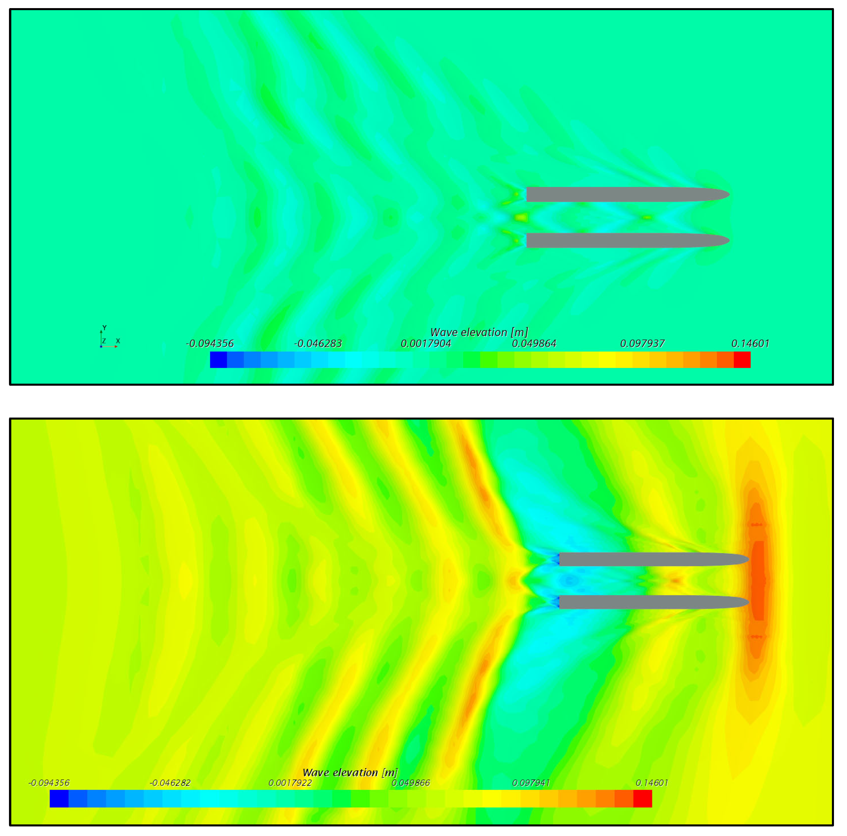
3.4. Wave-Making Resistance Calculations
4. Conclusions
Author Contributions
Funding
Institutional Review Board Statement
Informed Consent Statement
Data Availability Statement
Acknowledgments
Conflicts of Interest
Nomenclature
| α | Constant |
| B, BM | Beam moulded (m) |
| CF, CF0 | Frictional drag coefficient |
| CT | Total drag coefficient |
| CT-CFD | Total drag coefficient by CFD |
| CT-Exp | Total drag coefficient by experiments |
| CT-Ext | Extrapolated total drag coefficient |
| ε | Relative Error (%) |
| λ | Model scale ratio |
| L, LPP | Length between perpendiculars (m) |
| LWL | Length of waterline (m) |
| υ | Kinematic viscosity (N s m−2) |
| Displacement volume (m3) | |
| r | Density of water (kg m−3) |
| P | Pressure (N m−2) |
| Q | Pitch Amplitude (deg) |
| R | Convergence Condition |
| S | Wetted hull surface area (m2) |
| T | Draught at Midship (m) |
| u, v, w | Fluid velocity components |
| y+ | Dimensionless wall distance |
| Z | Heave Amplitude (m) |
| ζ | Wave height (m) |
| (1 + k) | Form Factor |
| BCs | Boundary Conditions |
| CF | Correction Factor |
| CFD | Computational Fluid Dynamics |
| DC372 | Delft Catamaran 372 |
| DoF | Degree of Freedom |
| EFD | Experimental Fluid Dynamics |
| Fr, Fn | Froude Number |
| FS | Factors of Safety |
| GCI | Grid Convergence Index |
| H2020 | Horizon 2020 |
| HSVA | Hamburg Ship Model Basin |
| ITTC | International Towing Tank Conference |
| KB | Vertical Centre of Buoyancy |
| LC | Loading Condition |
| LCB | Longitudinal Centre of Buoyancy |
| RANS | Reynolds-averaged Navier–Stokes |
| TrAM | Transport: Advanced and Modular |
| WAM-V | Wave adaptive modular vessel |
| VoF | Volume of Fluid |
References
- Molland, A.; Wellicome, J.; Couser, P. Resistance Experiments on a Systematic Series of High Speed Displacement Catamaran Forms: Variation of Length-Displacement Ratio and Breadth-Draught Ratio; Ship Science Report No. 71; University of Southampton: Iskandar Puteri, Malaysia, 1994. [Google Scholar]
- Insel, M.; Doctors, L.J. Wave pattern prediction of monohulls and catamarans in a shallow-water canal by linearised theory. In Proceedings of the 12th Australian Fluid Mechanics Conference, Sydney, NSW, Australia, December 1995; pp. 259–262. Available online: https://www.afms.org.au/proceedings/12/Insel_and_Doctors_1995.pdf (accessed on 22 November 2022).
- Veer, R.V. Experimental Results of Motions, Hydrodynamic Coefficients and Wave Loads on the 372 Catamaran Model; Technical Report 1129; Delft University of Technology: Delft, The Netherlands, 1998. [Google Scholar]
- Castiglione, T.; He, W.; Stern, F.; Bova, S. Effects of shallow water on catamaran interference. In Proceedings of the 11th International Conference on FAST2011, Honolulu, HI, USA; 26–29 September 2011. [Google Scholar]
- Milanov, E.; Chotukova, V.; Stern, F. System Based Simulation of Delft372 Catamaran Maneuvering Characteristics as Function of Water Depth and Approach Speed. In Proceedings of the 29th Symposium on Naval Hydrodynamics, Gothenburg, Sweden, 26–31 August 2012. [Google Scholar]
- Broglia, R.; Jacob, B.; Zaghi, S.; Stern, F.; Olivieri, A. Experimental investigation of interference effects for high-speed catamarans. Ocean. Eng. 2014, 76, 75–85. [Google Scholar] [CrossRef]
- Begovic, E. Wave Interference Prediction of a Trimaran Using Form Factor. In HSMV 2020: Proceedings of the 12th Symposium on High Speed Marine Vehicles; IOS Press: Amsterdam, The Netherlands; Volume 5, p. 99.
- Bašić, J.; Blagojević, B.; Andrun, M. Improved estimation of ship wave-making resistance. Ocean. Eng. 2020, 200, 107079. [Google Scholar] [CrossRef]
- Papanikolaou, A.; Xing-Kaeding, Y.; Strobel, J.; Kanellopoulou, A.; Zaraphonitis, G.; Tolo, E. Numerical and Experimental Optimization Study on a Fast, Zero Emission Catamaran. JMSE 2020, 8, 657. [Google Scholar] [CrossRef]
- Boulougouris, E.; Papanikolaou, A.; Dahle, M.; Tolo, E.; Xing-Kaeding, Y.; Jürgenhake, C.; Seidenberg, T.; Sachs, C.; Brown, C.; Jenset, F. Implementation of Zero Emission Fast Shortsea Shipping. In Proceedings of the SNAME Maritime Convention; Online, 27–29 October 2021. [Google Scholar]
- Shi, G. Numerical investigation of the resistance of a zero-emission full-scale fast catamaran in shallow water. J. Mar. Sci. Eng. 2021, 9, 563. [Google Scholar] [CrossRef]
- Duman, S.; Bal, S. Turn and zigzag manoeuvres of Delft catamaran 372 using CFD-based system simulation method. Ocean. Eng. 2022, 264, 112265. [Google Scholar] [CrossRef]
- Ulgen, K.; Dhanak, M.R. Hydrodynamic Performance of a Catamaran in Shallow Waters. J. Mar. Sci. Eng. 2022, 10, 1169. [Google Scholar] [CrossRef]
- TrAM. Transport: Advanced and Modular (TrAM) Horizon2020 Project. 2022. Available online: https://tramproject.eu/ (accessed on 22 November 2022).
- Simcenter STAR-CCM+. 2022. Available online: https://www.plm.automation.siemens.com/global/en/products/simcenter/STAR-CCM.html (accessed on 22 November 2022).
- Hirt, C.W.; Nichols, B.D. Volume of fluid (VOF) method for the dynamics of free boundaries. J. Comput. Phys. 1981, 39, 201–225. [Google Scholar] [CrossRef]
- ITTC. Practical Guidelines for Ship CFD Applications. In Proceedings of the 26th ITTC, Rio de Janerio, Brazil. 2011. Available online: https://ittc.info/media/1357/75-03-02-03.pdf (accessed on 22 November 2022).
- Benek, J.A.; Steger, J.L.; Dougherty, F.C.; Buning, P.G. Chimera: A Grid-Embedding Technique. AEDC-TR-85-64; Arnold Engineering Development Center: Fort Belvoir, VA, USA, 1986. [Google Scholar]
- Begovic, E. Pure Yaw Simulations of Fast Delft Catamaran 372 in Deep Water. In HSMV 2020: Proceedings of the 12th Symposium on High Speed Marine Vehicles; IOS Press: Amsterdam, The Netherlands; Volume 5, p. 109.
- Duman, S.; Bal, S. Prediction of maneuvering coefficients of Delft catamaran 372 hull form. In Sustainable Development and Innovations in Marine Technologies, 1st ed.; Georgiev, P., Soares, C.G., Eds.; CRC Press: Boca Raton, FL, USA, 2019; pp. 167–174. [Google Scholar] [CrossRef]
- Prohaska, C. A simple method for the evaluation of the form factor and the low speed wave resistance. In Hydro-and Aerodynamics Laboratory, Lyngby, Denmark, Hydrodynamics Section, Proceedings of the 11th International Towing Tank Conference, ITTC’66; Resistance Committee: Tokyo, Japan, 1966; pp. 65–66. [Google Scholar]
- Hughes, G. Friction and form resistance in turbulent flow, and a proposed formulation for use in model and ship correlation. In National Physical Laboratory, NPL, Ship Division, Presented at the Institution of Naval Architects, Paper no. 7, RINA Transactions, London; April 1954. Available online: https://repository.tudelft.nl/islandora/object/uuid%3A9a642c53-27f0-45fe-a5e4-5e1296b62af1 (accessed on 22 November 2022).
- ITTC. Report of 8th ITTC Resistance Committee. In Proceedings of the 8th International Towing Tank Conference, Madrid, Spain, September 1957. Available online: https://repository.tudelft.nl/islandora/object/uuid%3A4aa44007-881c-441c-82dd-70f45cc70ff2 (accessed on 22 November 2022).
- Roache, P.J. Perspective: A Method for Uniform Reporting of Grid Refinement Studies. J. Fluids Eng. 1994, 116, 405. [Google Scholar] [CrossRef]
- Stern, F.; Wilson, R.V.; Coleman, H.W.; Paterson, E.G. Comprehensive Approach to Verification and Validation of CFD Simulations—Part 1: Methodology and Procedures. J. Fluids Eng. 2001, 123, 793. [Google Scholar] [CrossRef]
- Celik, I.B.; Ghia, U.; Roache, P.J.; Freitas, C.J. Procedure for Estimation and Reporting of Uncertainty Due to Discretization in CFD Applications. J. Fluids Eng. 2008, 130, 078001. [Google Scholar] [CrossRef]
- Xing, T.; Stern, F. Factors of Safety for Richardson Extrapolation. J. Fluids Eng. 2010, 132, 061403. [Google Scholar] [CrossRef]
- ITTC. Resistance, Uncertainty Analysis, Example for Resistance Test. In Proceedings of the International Towing Tank Conference. 2002. Available online: https://ittc.info/media/1818/75-02-02-02.pdf (accessed on 22 November 2022).
- Phillips, T.S.; Roy, C.J. Richardson Extrapolation-Based Discretization Uncertainty Estimation for Computational Fluid Dynamics. J. Fluids Eng. 2014, 136, 121401. [Google Scholar] [CrossRef]
- Korkmaz, K.B. CFD based form factor determination method. Ocean. Eng. 2021, 220, 108451. [Google Scholar] [CrossRef]


| Dimension | Nondim. | Nondim. Value |
|---|---|---|
| Separation (s) | s/Lpp | 0.227 |
| Draught (T) | T/Lpp | 0.040 |
| KB | KB/Lpp | 0.026 |
| LCB | LCB/Lpp | 0.460 |
| Boundaries | Background (× L) | Overset (× L) |
|---|---|---|
| Upstream | 2.370 | 0.072 |
| Downstream | 3.745 | 0.037 |
| Top | 1.685 | 0.169 |
| Bottom | 1.685 | 0.015 |
| Side | 2.247 | 0.187 |
| Grid Quality | Total Cell Numbers | CT (1 × 10³) |
|---|---|---|
| Fine | 8.36 × 10⁶ | 6.345 |
| Medium | 4.82 × 10⁶ | 6.512 |
| Coarse | 2.92 × 10⁶ | 6.648 |
| GCI | CF | FS | |
|---|---|---|---|
| r21 | 1.20 | 1.20 | 1.20 |
| r32 | 1.18 | 1.18 | 1.18 |
| R | 0.73 | 0.73 | 0.73 |
| Pth | 2.00 | 2.00 | 2.00 |
| PRE | 2.19 | 2.19 | 2.19 |
| CT-Ext (1 × 10³) | 6.213 | 6.213 | 6.213 |
| SF | 1.25 | 1.12 | 1.10 |
| Δ (%) | 3.90 | 3.86 | 10.01 |
| Fr | CT-CFD (1 × 10³) | CT-Exp (1 × 10³) | CF-CFD (1 × 10³) | CF-Exp (1 × 10³) | ||
|---|---|---|---|---|---|---|
| 0.24 | 5.064 | 4.917 | −2.98% | 3.248 | 3.071 | −5.75% |
| 0.33 | 5.002 | 4.876 | −2.59% | 3.089 | 2.906 | −6.31% |
| 0.39 | 5.332 | 5.161 | −3.32% | 3.028 | 2.825 | −7.21% |
| 0.45 | 6.345 | 6.488 | 2.21% | 2.947 | 2.758 | −6.87% |
| 0.51 | 6.125 | 6.281 | 2.48% | 2.837 | 2.701 | −5.01% |
| 0.57 | 5.461 | 5.552 | 1.65% | 2.756 | 2.652 | −3.91% |
| 0.63 | 4.854 | 4.933 | 1.60% | 2.720 | 2.610 | −4.24% |
| Fr | Z′CFD (1 × 10³) | QCFD (deg) | Z′Exp (1 × 10³) | QExp (Deg) |
|---|---|---|---|---|
| 0.24 | −0.710 | 0.052 | −0.635 | −0.033 |
| 0.33 | −1.649 | −0.026 | −1.404 | −0.117 |
| 0.39 | −2.436 | −0.218 | −2.273 | −0.300 |
| 0.45 | −3.276 | −0.879 | −2.774 | −1.133 |
| 0.51 | −2.694 | −1.245 | −1.872 | −1.517 |
| 0.57 | −1.763 | −1.258 | −0.869 | −1.483 |
| 0.63 | −0.779 | −1.124 | −0.267 | −1.317 |
| Fn | CT-DW (1 × 10³) | CF-DW (1 × 10³) | CT-SW (1 × 10³) | CF-SW (1 × 10³) | ||
|---|---|---|---|---|---|---|
| 0.20 | 4.233 | 3.026 | 6.952 | 3.369 | −64.2% | −11.3% |
| 0.24 | 4.634 | 3.024 | 17.720 | 3.817 | −282.4 | −26.2 |
| 0.27 | 4.601 | 2.959 | 14.657 | 3.206 | −218.6 | −8.3 |
| 0.30 | 4.875 | 2.943 | 11.362 | 2.830 | −133.1 | 3.8 |
| 0.33 | 4.545 | 2.920 | 9.707 | 2.726 | −113.6 | 6.6 |
| 0.36 | 4.377 | 2.886 | 8.212 | 2.684 | −87.6 | 7.0 |
| 0.39 | 4.973 | 2.873 | 6.900 | 2.664 | −38.8 | 7.3 |
| 0.45 | 6.066 | 2.810 | 5.515 | 2.615 | 9.1 | 7.0 |
| 0.51 | 5.872 | 2.717 | 4.864 | 2.607 | 17.2 | 4.1 |
| 0.57 | 5.368 | 2.665 | 4.492 | 2.574 | 16.3 | 3.4 |
| 0.63 | 4.924 | 2.630 | 4.244 | 2.580 | 13.8 | 1.9 |
| 0.66 | 4.773 | 2.614 | 4.189 | 2.592 | 12.2 | 0.8 |
| Fn | Z′DW (1 × 10³) | Z′SW (1 × 10³) | QDW (Deg) | QSW (Deg) |
|---|---|---|---|---|
| 0.20 | 0.0788 | −1.3383 | 0.0709 | 0.0235 |
| 0.24 | 0.1690 | −5.0447 | 0.0390 | −1.6505 |
| 0.27 | −0.0017 | −0.3331 | 0.0759 | −1.7179 |
| 0.30 | −0.3753 | 2.6961 | 0.0177 | −1.4326 |
| 0.33 | −0.6346 | 4.4842 | 0.0222 | −1.5421 |
| 0.36 | −0.9065 | 3.9456 | 0.0637 | −1.3896 |
| 0.39 | −1.5303 | 4.0002 | −0.1157 | −1.1658 |
| 0.45 | −2.4447 | 4.1026 | −0.8402 | −0.8632 |
| 0.51 | −1.7202 | 4.1489 | −1.1490 | −0.6744 |
| 0.57 | −1.0439 | 4.2890 | −1.1295 | −0.5704 |
| 0.63 | −0.0822 | 4.2859 | −0.9756 | −0.4221 |
| 0.66 | 0.3753 | 4.2635 | −0.9136 | −0.3666 |
| Fn | FFSW | CW-SW | FFDW | CW-DW |
|---|---|---|---|---|
| 0.20 | 1.3406 | 2.41 × 10³ | 1.3128 | 3.40 × 10⁴ |
| 0.24 | 1.3489 | 1.26 × 10² | 1.3219 | 6.36 × 10⁴ |
| 0.27 | 1.3545 | 1.03 × 10² | 1.3266 | 6.75 × 10⁴ |
| 0.30 | 1.3601 | 7.51 × 10³ | 1.3334 | 9.51 × 10⁴ |
| 0.33 | 1.3644 | 5.99 × 10³ | 1.3393 | 6.35 × 10⁴ |
| 0.36 | 1.3712 | 4.53 × 10³ | 1.3463 | 4.92 × 10⁴ |
| 0.39 | 1.3762 | 3.23 × 10³ | 1.3490 | 1.10 × 10³ |
| 0.45 | 1.3853 | 1.89 × 10³ | 1.3512 | 2.27 × 10³ |
| 0.51 | 1.3936 | 1.23 × 10³ | 1.3583 | 2.18 × 10³ |
| 0.57 | 1.4008 | 8.86 × 10⁴ | 1.3673 | 1.72 × 10³ |
| 0.63 | 1.4076 | 6.12 × 10⁴ | 1.3870 | 1.28 × 10³ |
| 0.66 | 1.4104 | 5.33 × 10⁴ | 1.3910 | 1.14 × 10³ |
Disclaimer/Publisher’s Note: The statements, opinions and data contained in all publications are solely those of the individual author(s) and contributor(s) and not of MDPI and/or the editor(s). MDPI and/or the editor(s) disclaim responsibility for any injury to people or property resulting from any ideas, methods, instructions or products referred to in the content. |
© 2023 by the authors. Licensee MDPI, Basel, Switzerland. This article is an open access article distributed under the terms and conditions of the Creative Commons Attribution (CC BY) license (https://creativecommons.org/licenses/by/4.0/).
Share and Cite
Duman, S.; Boulougouris, E.; Aung, M.Z.; Xu, X.; Nazemian, A. Numerical Evaluation of the Wave-Making Resistance of a Zero-Emission Fast Passenger Ferry Operating in Shallow Water by Using the Double-Body Approach. J. Mar. Sci. Eng. 2023, 11, 187. https://doi.org/10.3390/jmse11010187
Duman S, Boulougouris E, Aung MZ, Xu X, Nazemian A. Numerical Evaluation of the Wave-Making Resistance of a Zero-Emission Fast Passenger Ferry Operating in Shallow Water by Using the Double-Body Approach. Journal of Marine Science and Engineering. 2023; 11(1):187. https://doi.org/10.3390/jmse11010187
Chicago/Turabian StyleDuman, Suleyman, Evangelos Boulougouris, Myo Zin Aung, Xue Xu, and Amin Nazemian. 2023. "Numerical Evaluation of the Wave-Making Resistance of a Zero-Emission Fast Passenger Ferry Operating in Shallow Water by Using the Double-Body Approach" Journal of Marine Science and Engineering 11, no. 1: 187. https://doi.org/10.3390/jmse11010187
APA StyleDuman, S., Boulougouris, E., Aung, M. Z., Xu, X., & Nazemian, A. (2023). Numerical Evaluation of the Wave-Making Resistance of a Zero-Emission Fast Passenger Ferry Operating in Shallow Water by Using the Double-Body Approach. Journal of Marine Science and Engineering, 11(1), 187. https://doi.org/10.3390/jmse11010187