

Research on the Karhunen–Loève Transform Method and Its Application to Hull Form Optimization

Abstract
1. Introduction
2. K–L Transform Method
2.1. Basic Principle of K–L Transform
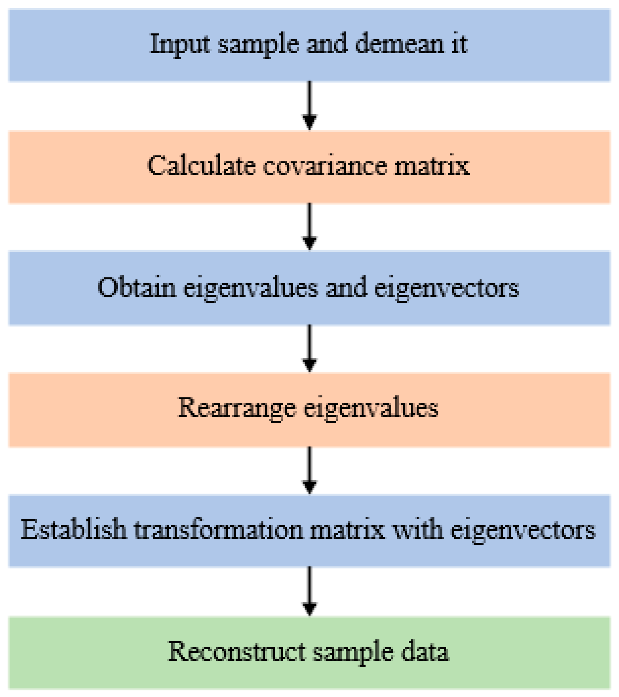
2.2. K–L Transform–Based Data Dimensionality Reduction Process
- (1)
- An M × N sample dataset (where M and N are the numbers of samples and feature dimensions, respectively) is demeaned.
- (2)
- The covariance matrix of the demeaned sample data matrix is calculated.
- (3)
- The eigenvalues and eigenvectors of the resulting N × N covariance matrix are calculated.
- (4)
- The eigenvalues are arranged in a descending order, and their corresponding eigenvectors are arranged in a corresponding order.
- (5)
- A threshold is assigned to β. If the ratio of the sum of the K (K < N) largest eigenvalues to the sum of all eigenvalues (feature contribution rate) is larger than the threshold, the dimensionality of the original data can be reduced to K. An N × K transformation matrix is established using the eigenvectors corresponding to the largest K eigenvalues.
- (6)
- An M × K matrix is obtained by multiplying the normalized M × N sample data matrix with the N × K transformation matrix, thereby reducing the dimensionality of the sample data matrix from N to K.
3. Methods for Eigenvalue of Matrix
3.1. Jacobi Iteration Method
3.2. Rapid PCA Method
4. K–L Transform–Based Hull Form Reconstruction Method
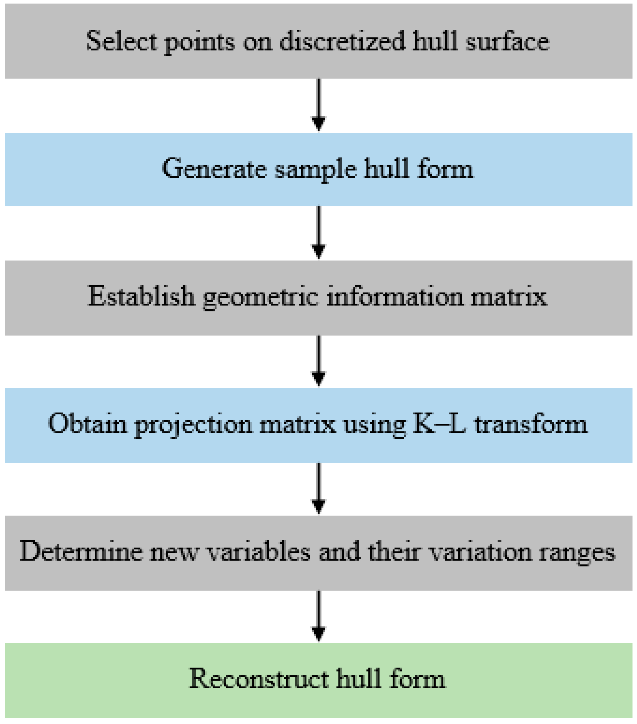
4.1. Hull Form Reconstruction Process
- (1)
- (2)
- A certain number of samples are collected using the uniform experimental design method to generate a sample offset matrix and the corresponding hull forms using the RBF-based shape modification method.
- (3)
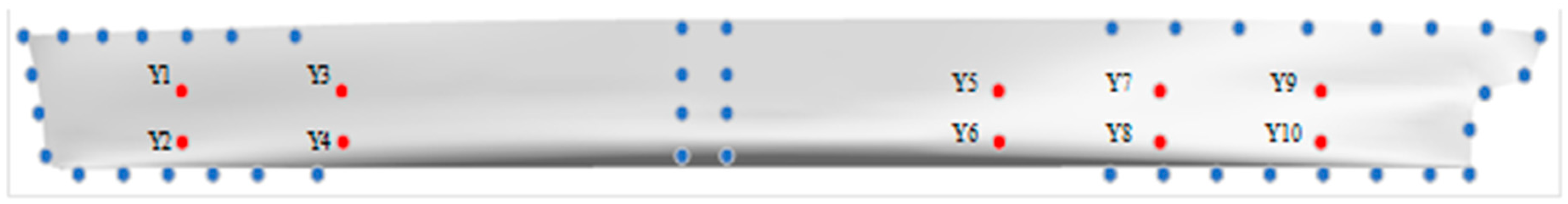
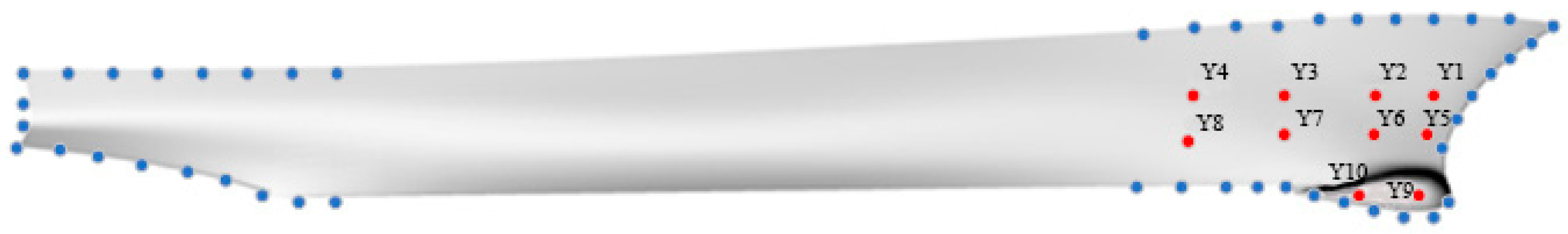
- For each sample hull form generated, M offset points are selected, and their x-, y-, and z-coordinates are arranged in a geometric information matrix.
- (4)
- The covariance matrix of the demeaned geometric information matrix is calculated using the K–L transform method to obtain its eigenvalues and eigenvectors. The eigenvectors are arranged according to the eigenvalues, and a threshold of β is assigned to generate a transformation matrix. The sample offset matrix is normalized and multiplied with the transformation matrix to produce a projection matrix.
- (5)
- The new design variables in the dimensionality-reduced projection matrix and their respective variation ranges are defined.
- (6)
- Hull form reconstruction is performed using the hull form reconstruction equations to obtain the hull offset matrix and generate the corresponding hull form.
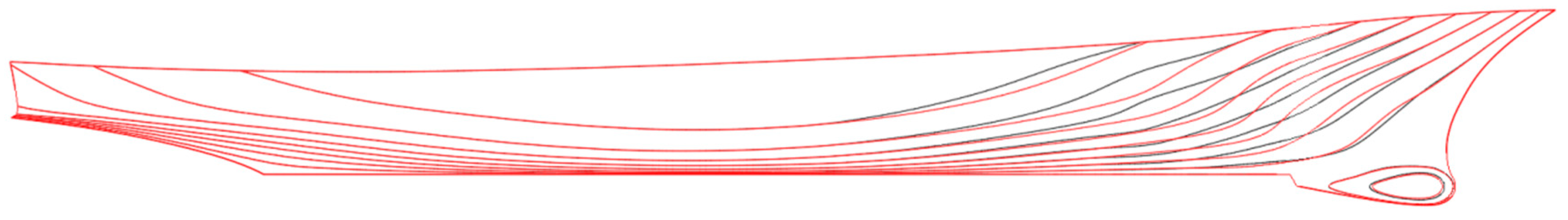
4.2. Examples of Hull Form Reconstruction
5. Optimization of Wave-Making Resistance Coefficient for DTMB 5415
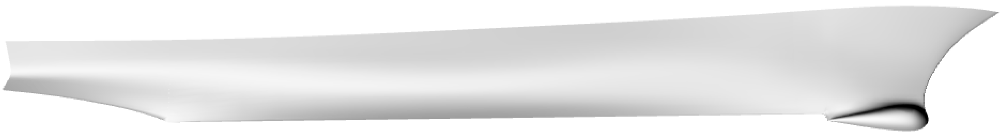
5.1. Optimized Object
5.2. Description of Optimization Problem
- (1)
- Objective of optimization
- (2)
- Setting of optimization variables
- (3)
- Constraint conditions.
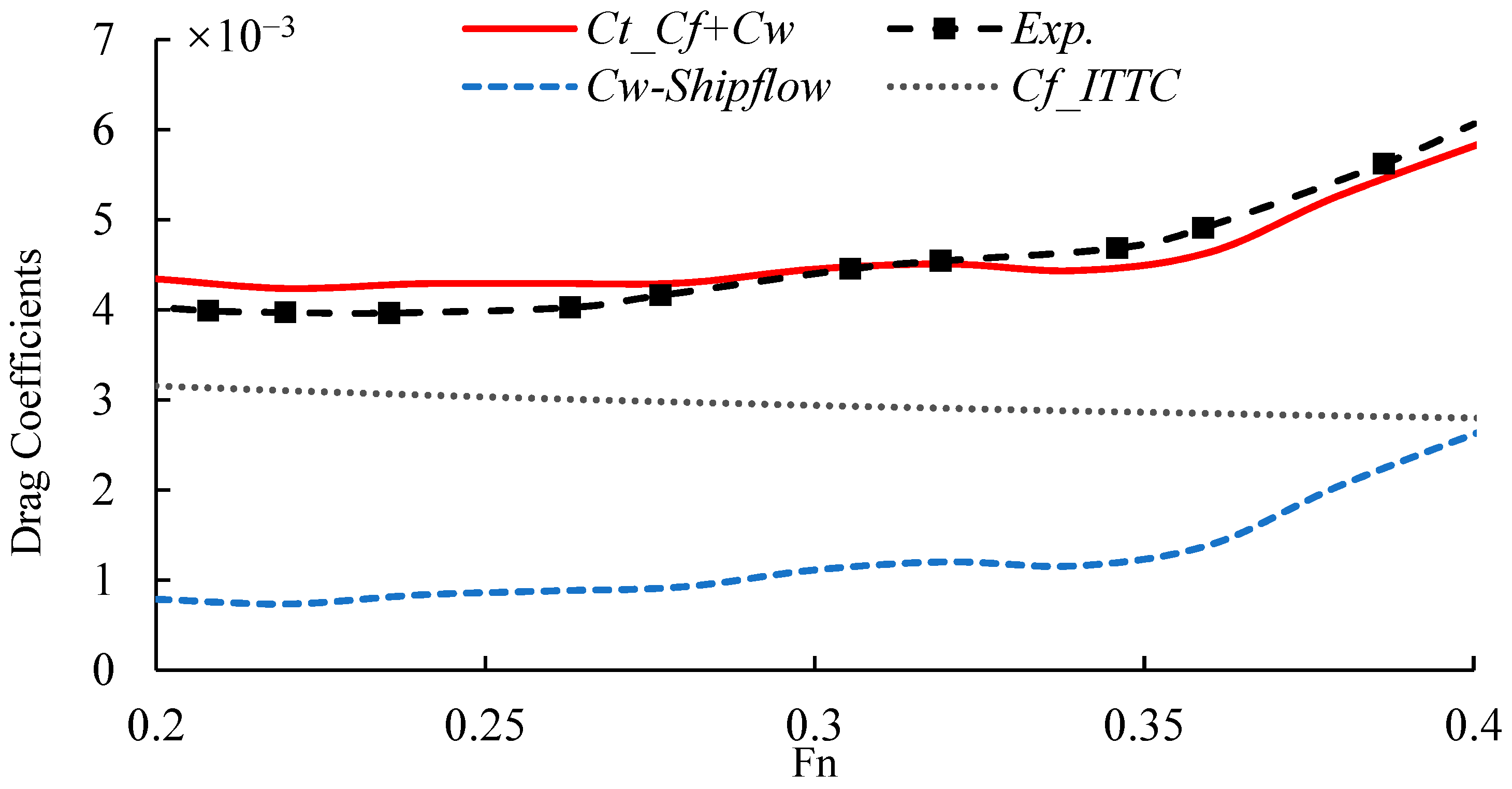
5.3. CFD Simulation
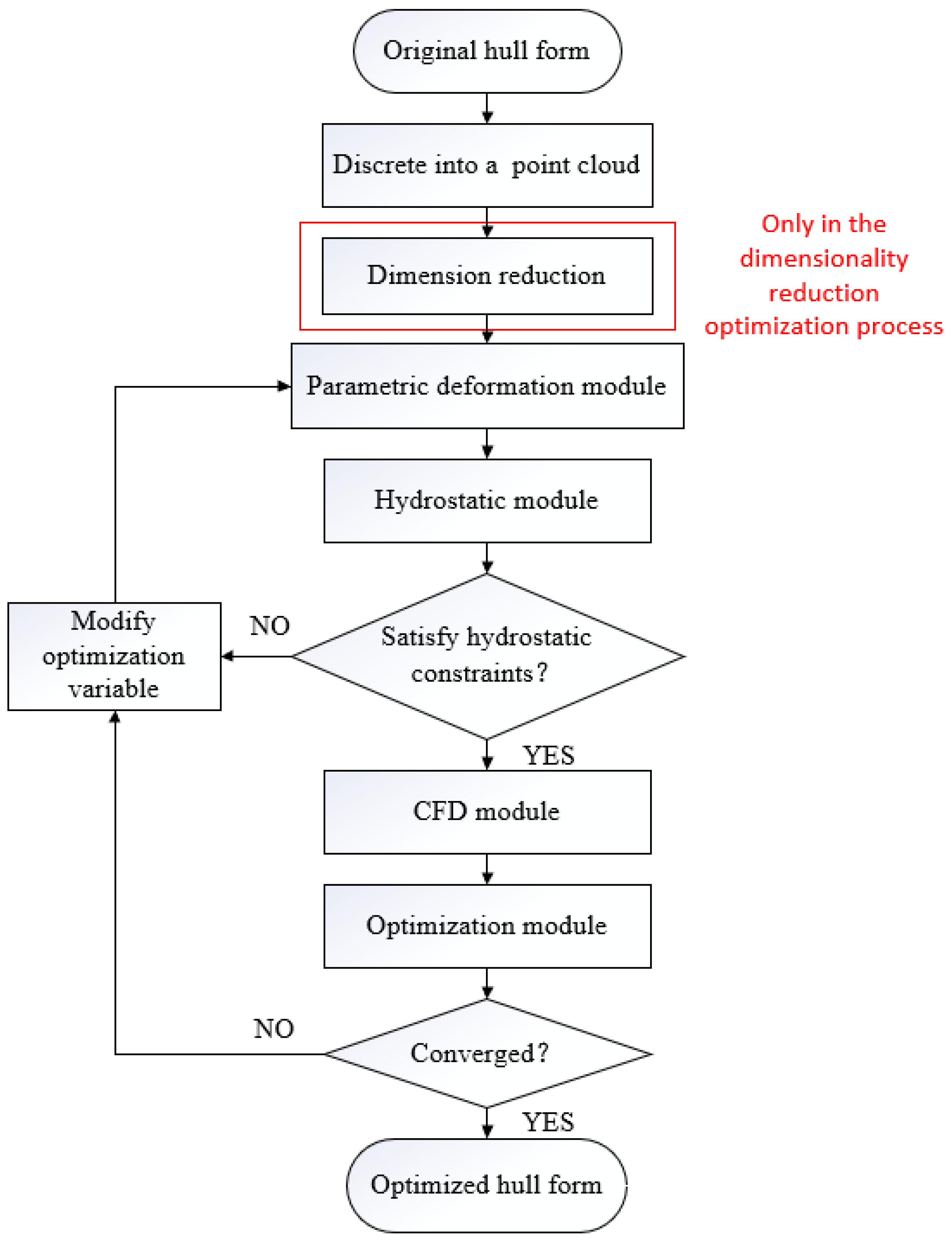
5.4. Optimization Process
- (1)
- Direct optimization process
- (2)
- Dimensionality reduction optimization process
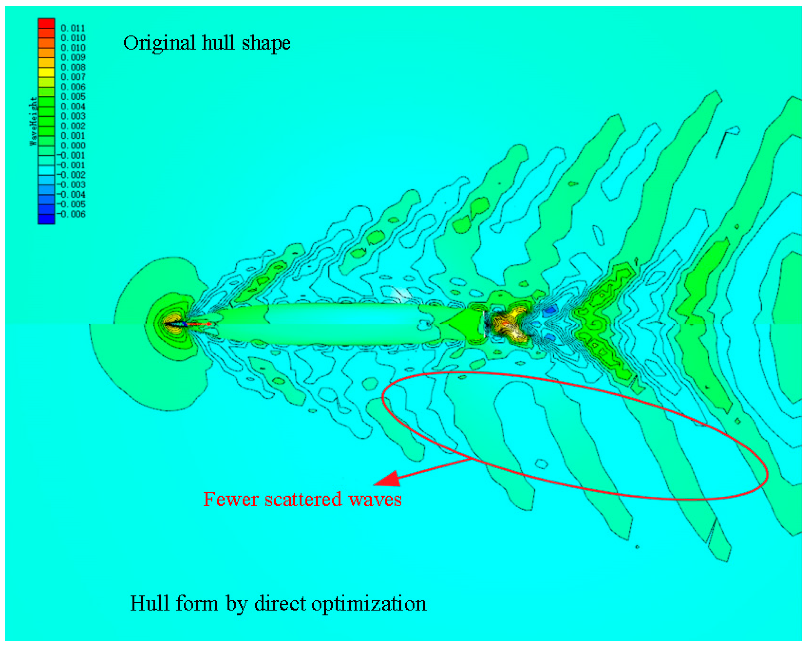
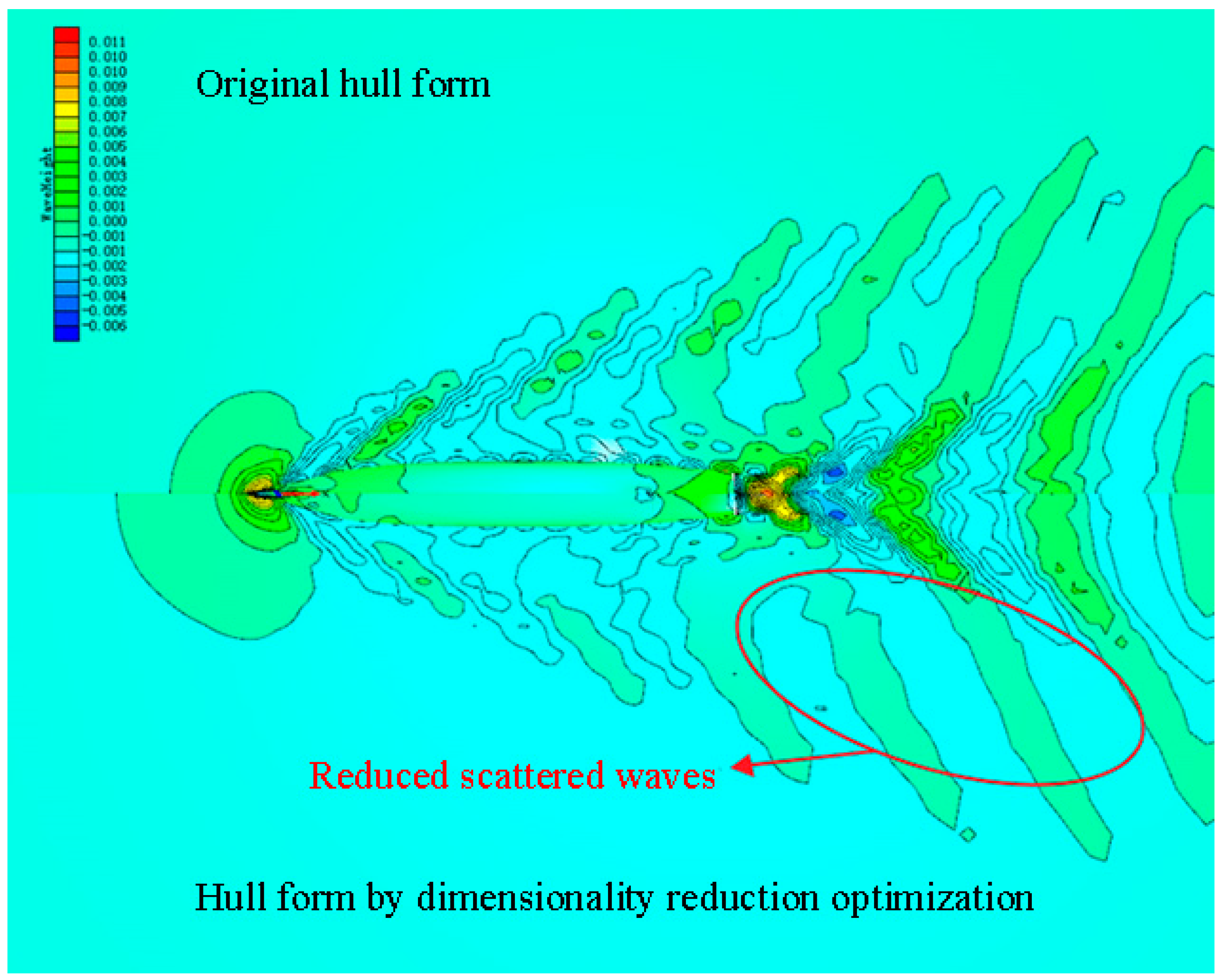
5.5. Optimization Results
- (1)
- Results of direct optimization
- (2)
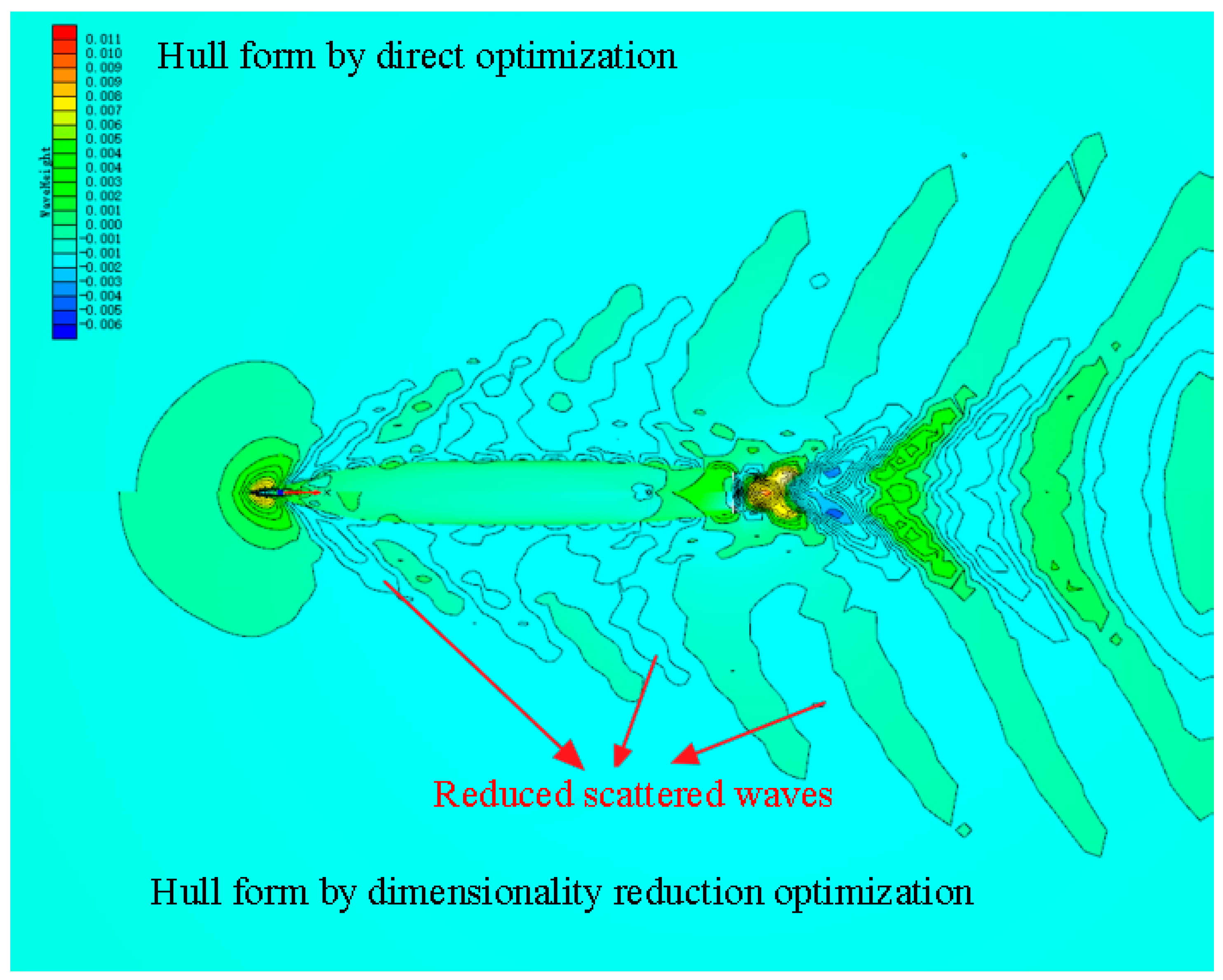
- Results of dimensionality reduction optimization
- (3)
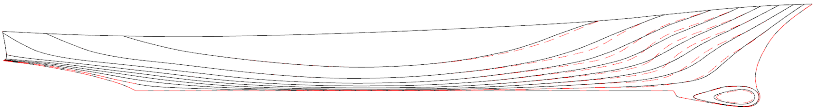
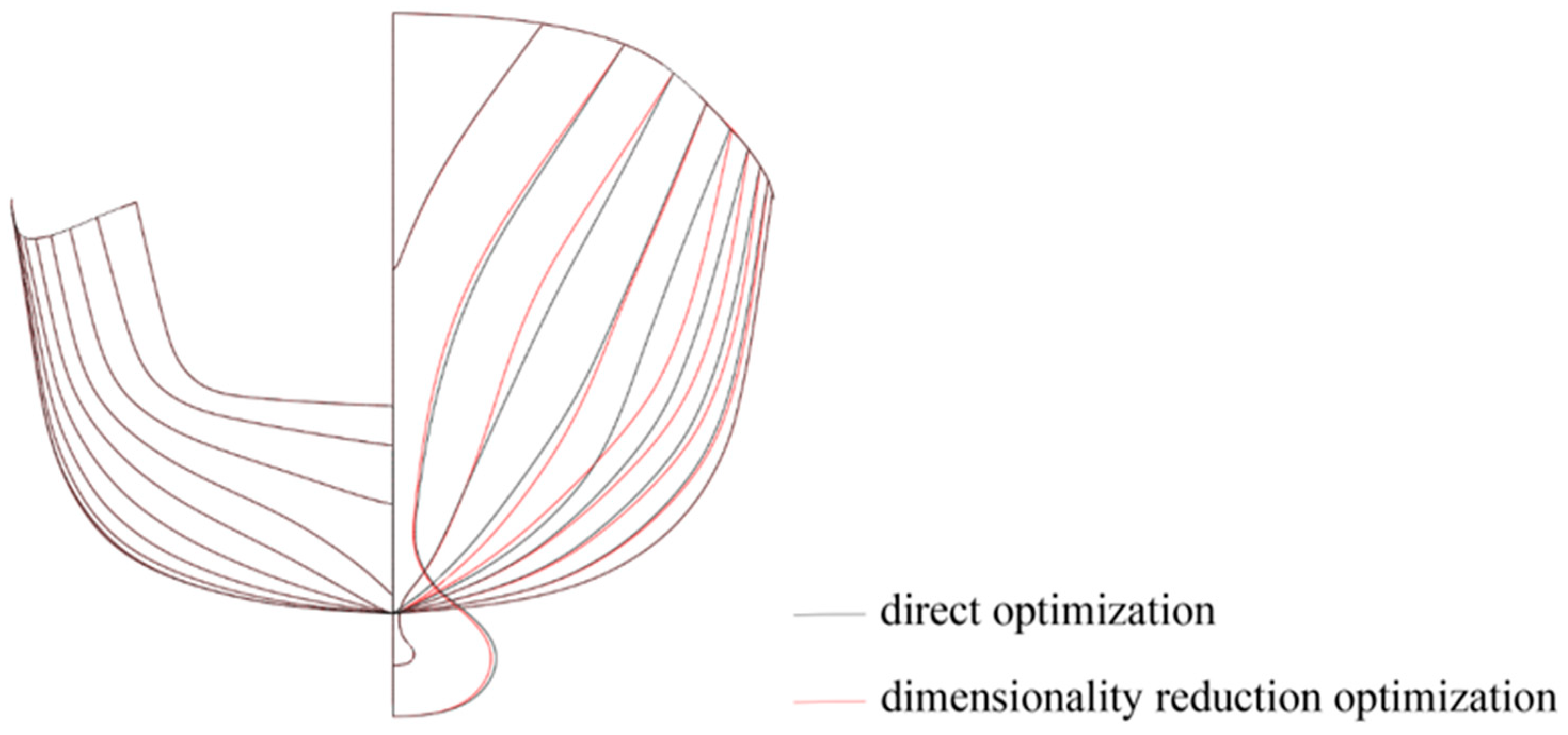
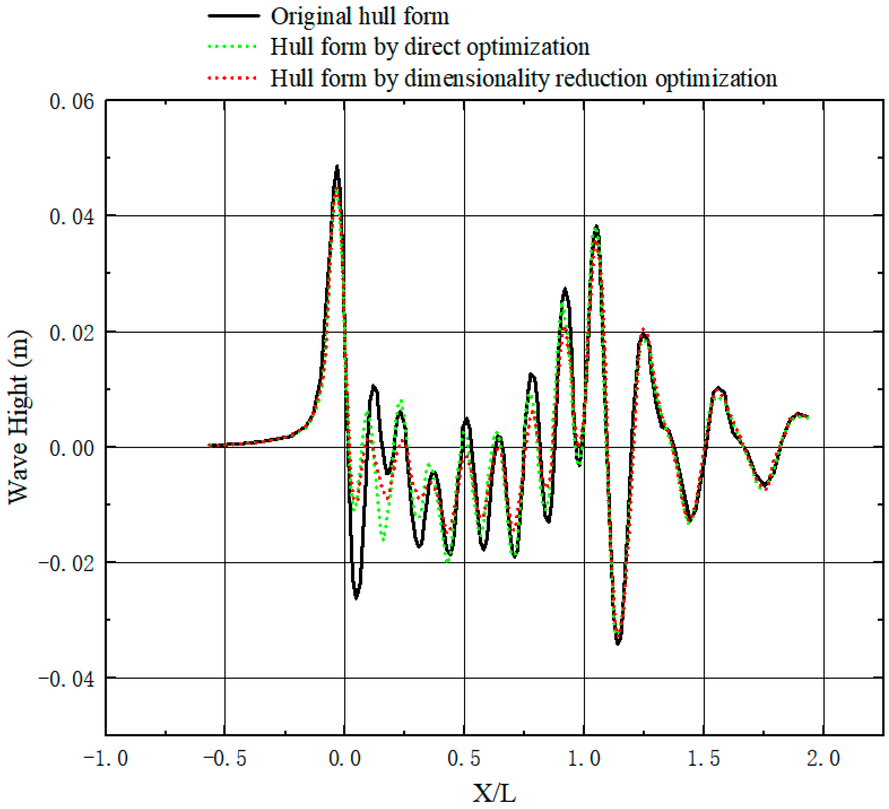
- Comparison of direct and dimensionality reduction optimization results.
6. Conclusions
- (1)
- The K–L transform is a linear dimensionality reduction method and assumes the presence of a linear relationship between data. Thus, its dimensionality reduction performance could be limited on nonlinear data. This study did not investigate the application of nonlinear dimensionality reduction methods, which will be tested in the future.
- (2)
- To reduce the computation time, the sample data used in the dimensionality reduction optimization performed in this study only included the geometric information of the hull and excluded its physical information. The consideration of physical information requires a detailed computation of the ship performance in the early stage, and the physical information of a new hull form can be directly obtained by dimensionality reduction reconstruction. This is a major direction for future research.
Author Contributions
Funding
Institutional Review Board Statement
Informed Consent Statement
Data Availability Statement
Conflicts of Interest
Nomenclature
| m | the waterline length | |
| m | the longitudinal center of buoyancy | |
| m | the maximum waterplane width | |
| m | ||
| / | the block coefficient | |
| / | the fullest cross-section area | |
| m3 | the volume of displacement | |
| m2 | the wetted surface area | |
| Fr | / | Froude number |
| Rw | N | the wave-making resistance |
| Cw | / | the wave-making resistance coefficient |
References
- Cheng, X.; Li, G.; Skulstad, R. Data-driven uncertainty and sensitivity analysis for ship motion modeling in offshore operations. Ocean Eng. 2019, 179, 261–272. [Google Scholar] [CrossRef]
- Hu, H.; Zhang, G.; Li, D. Shape optimization of airfoil in ground effect based on free-form deformation utilizing sensitivity analysis and surrogate model of artificial neural network. Ocean Eng. 2022, 257, 514–527. [Google Scholar] [CrossRef]
- Guan, G.; Yang, Q.; Gu, W. A new method for parametric design and optimization of ship inner shell based on the improved particle swarm optimization algorithm. Ocean Eng. 2018, 169, 551–566. [Google Scholar] [CrossRef]
- Hamed, A. Multi-objective optimization method of trimaran hull form for resistance reduction and propeller intake flow improvement. Ocean Eng. 2022, 244, 352–366. [Google Scholar] [CrossRef]
- Jung, Y.-W.; Kim, Y. Hull form optimization in the conceptual design stage considering operational efficiency in waves. Proc. Inst. Mech. Eng. Part M J. Eng. Marit. Environ. 2019, 233, 745–759. [Google Scholar] [CrossRef]
- Liu, Q.; Feng, B.; Liu, Z.; Zhang, H. The improvement of a variance-based sensitivity analysis method and its application to a ship hull optimization model. J. Mar. Sci. Technol. 2017, 22, 694–709. [Google Scholar] [CrossRef]
- Guan, G.; Zhuang, Z.; Yang, Q. Design parameter sensitivity analysis for SWATH with minimum resistance at design and service speeds. Ocean Eng. 2021, 240, 961–972. [Google Scholar] [CrossRef]
- Jeon, M.; Yoon, H.K.; Hwang, J. Analysis of the dynamic characteristics for the change of design parameters of an underwater vehicle using sensitivity analysis. Int. J. Nav. Archit. Ocean Eng. 2018, 10, 508–519. [Google Scholar] [CrossRef]
- Coppedè, A.; Gaggero, S.; Vernengo, G. Hydrodynamic shape optimization by high fidelity CFD solver and Gaussian process based response surface method. Appl. Ocean Res. 2019, 90, 841–851. [Google Scholar] [CrossRef]
- Fu, X.; Lei, L.; Yang, G. Multi-objective shape optimization of autonomous underwater glider based on fast elitist non-dominated sorting genetic algorithm. Ocean Eng. 2018, 157, 339–349. [Google Scholar] [CrossRef]
- Yue, Y.; Han, C.; Cui, Y. TSP wavefield separation and noise suppression based on the LC-KL-DSW method. J. Appl. Geophys. 2022, 197, 552–560. [Google Scholar] [CrossRef]
- Fan, Y.; Xu, K.; Wu, H. Spatiotemporal Modeling for Nonlinear Distributed Thermal Processes Based on KL Decomposition, MLP and LSTM Network. IEEE Access 2020, 8, 11–21. [Google Scholar] [CrossRef]
- Ahuja, R.; Lall, B.; Prasad, S. On impropriety for a large-sized discrete fourier transform of a real-valued stationary process. Signal Process. 2022, 193, 397–402. [Google Scholar] [CrossRef]
- Trudu, M.; Pilia, M.; Hellbourg, G.; Pari, P.; Antonietti, N.; Maccone, C.; Melis, A.; Perrodin, D.; Trois, A. Performance analysis of the Karhunen–Loève Transform for artificial and astrophysical transmissions: Denoizing and detection. Mon. Not. R. Astron. Soc. 2020, 494, 69–83. [Google Scholar] [CrossRef]
- Siripatana, A.; Le Maitre, O.; Knio, O. Bayesian inference of spatially varying Manning’s n coefficients in an idealized coastal ocean model using a generalized Karhunen-Loève expansion and polynomial chaos. Ocean Dyn. 2020, 70, 1103–1127. [Google Scholar] [CrossRef]
- Reed, R.L.; Roberts, J.A. Application of the Karhunen-Loève Transform to the C5G7 benchmark in the response matrix method. Ann. Nucl. Energy 2017, 103, 350–355. [Google Scholar] [CrossRef]
- Allaix, D.L.; Carbone, V.I. An efficient coupling of FORM and Karhunen–Loève series expansion. Eng. Comput. 2016, 32, 1–13. [Google Scholar] [CrossRef]
- Azevedo, J.S.; Wisniewski, F.; Oliveira, S.P. A Galerkin method with two-dimensional Haar basis functions for the computation of the Karhunen–Loève expansion. Comput. Appl. Math. 2018, 37, 1825–1846. [Google Scholar] [CrossRef]
- Liu, L.; Yan, J.; Zheng, X.; Peng, H.; Guo, D.; Qu, X. Karhunen-Loève transform for compressive sampling hyperspectral images. Opt. Eng. 2015, 54, 014106. [Google Scholar] [CrossRef]
- Ai, X. A note on Karhunen–Loève expansions for the demeaned stationary Ornstein–Uhlenbeck process. Stat. Probab. Lett. 2016, 117, 113–117. [Google Scholar] [CrossRef]
- Chowdhary, K.; Najm, H.N. Bayesian estimation of Karhunen–Loève expansions; A random subspace approach. J. Comput. Phys. 2016, 319, 280–293. [Google Scholar] [CrossRef]
- Feng, J.W.; Cen, S.; Li, C.F.; Owen, D.R.J. Statistical reconstruction and Karhunen-Loève expansion for multiphase random media. Int. J. Numer. Methods Eng. 2016, 105, 3–32. [Google Scholar] [CrossRef]
- Diez, M.; Campana, E.F.; Andstern, F. Design-space dimensionality reduction in shape optimization by Karhunen–Loève expansion. Comput. Methods Appl. Mech. Eng. 2015, 283, 1525–1544. [Google Scholar] [CrossRef]
- Diez, M.; Serani, A.; Campana, E.F. Design-Space Dimensionality Reduction for Single- and Multi-Disciplinary Shape Optimization. In Proceedings of the 17th AIAA/ISSMO Multidisciplinary Analysis and Optimization Conference, Washington, DC, USA, 13–17 June 2016. [Google Scholar]
- Diez, M.; Serani, A.; Stern, F. Combined Geometry and Physics Based Method for Design-space Dimensionality Reduction in Hydrodynamic Shape Optimization. In Proceedings of the 31st Symposium on Naval Hydrodynamics, Monterey, CA, USA, 11–16 September 2016. [Google Scholar]
- Hotelling, H. Note on Edgeworth’s Taxation Phenomenon and Professor Garver’s Additional Condition on Demand Functions. Econometrica 1933, 1, 408–409. [Google Scholar] [CrossRef]
- Hotelling, H.; Hotelling, F. A new analysis of duration of pregnancy data. Am. J. Obstet. Gynecol. 1932, 23, 643–657. [Google Scholar] [CrossRef]
- Hotelling, H. Demand Functions with Limited Budgets. Econometrica 1935, 3, 66–78. [Google Scholar] [CrossRef]
- Feng, B.; Zhan, C.; Liu, Z. Application of Basis Functions for Hull Form Surface Modification. J. Mar. Sci. Eng. 2021, 9, 1005. [Google Scholar] [CrossRef]
- Chang, H.; Zhan, C.; Liu, Z.; Cheng, X.; Feng, B. Dynamic sampling method for ship resistance performance optimisation based on approximated model. Ships Offshore Struct. 2021, 16, 386–396. [Google Scholar] [CrossRef]
- Cheng, X.; Feng, B.; Liu, Z. Hull surface modification for ship resistance performance optimization based on Delaunay triangulation. Ocean Eng. 2018, 153, 333–344. [Google Scholar] [CrossRef]
- Cheng, X.; Feng, B.; Chang, H. Multi-objective optimisation of ship resistance performance based on CFD. J. Mar. Sci. Technol. 2019, 24, 152–165. [Google Scholar] [CrossRef]
- Ouyang, X.; Chang, H.; Feng, B. Information Matrix-Based Adaptive Sampling in Hull Form Optimisation. J. Mar. Sci. Eng. 2021, 9, 973. [Google Scholar] [CrossRef]
- Qiang, Z.; Bai-Wei, F.; Zu-Yuan, L.; Hai-Chao, C.; Xiao, W. Optimization method for hierarchical space reduction method and its application in hull form optimization. Ocean Eng. 2022, 262, 112–129. [Google Scholar] [CrossRef]
- Qiang, Z.; Hai-Chao, C.; Bai-Wei, F.; Zu-Yuan, L.; Cheng-Sheng, Z. Research on knowledge-extraction technology in optimisation of ship-resistance performance. Ocean Eng. 2019, 179, 325–336. [Google Scholar] [CrossRef]


| Serial Number | ||||||||||
|---|---|---|---|---|---|---|---|---|---|---|
| Upper limit | 1.243 | 1.885 | 2.396 | 3.22 | 3.371 | 4.203 | 2.743 | 3.369 | 1.058 | 1.273 |
| Lower limit | 1.051 | 1.577 | 2.055 | 2.795 | 2.963 | 3.751 | 2.270 | 3.010 | 0.908 | 1.075 |
| Serial Number | 1 | 2 | 3 | 4 | 5 |
|---|---|---|---|---|---|
| Eigenvalue | 6.49 | 1.95 | 1.05 | 0.46 | 0.22 |
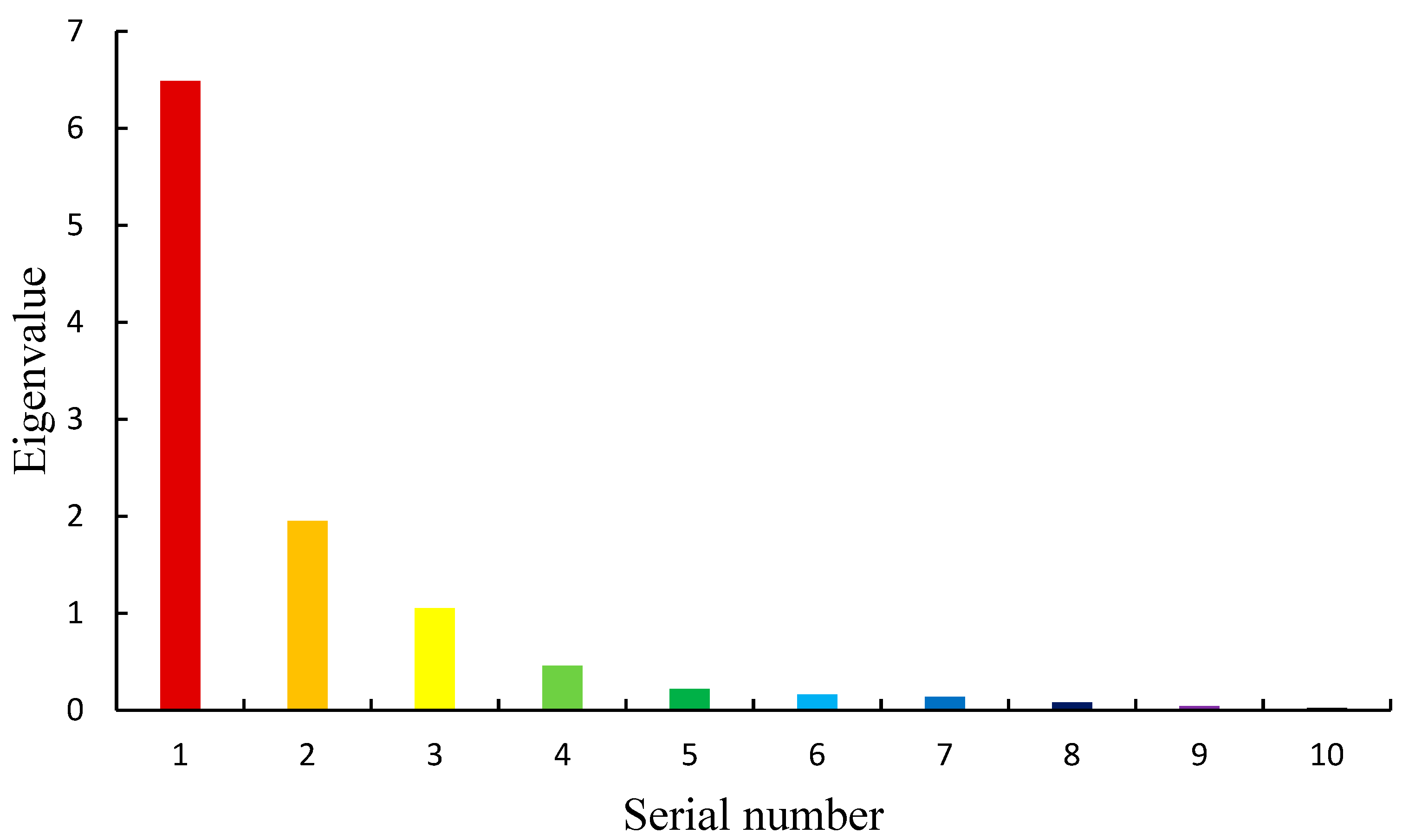
| Serial Number | 1 | 2 | 3 | 4 | 5 | 6 | 7 | 8 | 9 | 10 |
|---|---|---|---|---|---|---|---|---|---|---|
| Eigenvalue | 6.49 | 1.95 | 1.05 | 0.46 | 0.22 | 0.16 | 0.13 | 0.08 | 0.06 | 0.01 |
| 5.699 m | 3.293 m | 0.679 m | 0.248 m | 0.339 | 0.548 | 0.550 m3 | 4.904 m2 |
| Serial Number | ||||||||||
|---|---|---|---|---|---|---|---|---|---|---|
| Upper limit | 0.1325 | 0.1933 | 0.0955 | 0.0404 | 0.0629 | 0.1157 | 0.0152 | 0.0258 | 0.2100 | 0.2836 |
| Lower limit | 0.1104 | 0.1581 | 0.0801 | 0.0331 | 0.0514 | 0.0946 | 0.0125 | 0.0211 | 0.1860 | 0.2502 |
| Number of Iterations for Convergence | WMR Coefficient Cw (Variation %) | WMR Rw (Variation %) | |
|---|---|---|---|
| Original hull form | - | 6.83 × 10⁻⁴ | 4.647 N |
| Direct optimization | 3000 | 4.90 × 10⁻⁴ (−28.25%) | 3.328 N (−28.38%) |
| Volume of Displacement
(Variation %) | LCB Lcb (Variation %) | Wetted Surface Area Swet (Variation %) | |
|---|---|---|---|
| Original hull form | 0.550 m3 | 3.293 m | 4.904 m2 |
| Direct optimization | 0.553 m3 (+0.55%) | 3.286 m (−0.21%) | 4.903 m2 (−0.2%) |
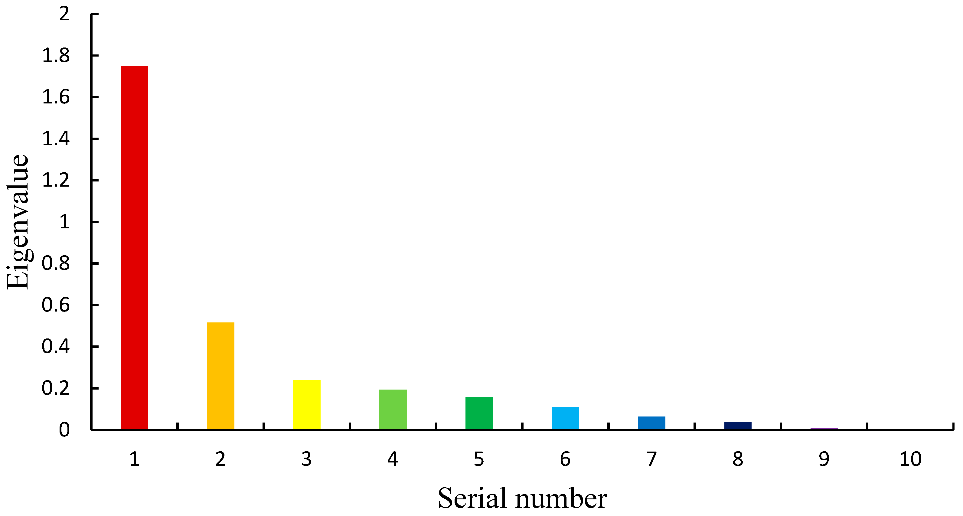
| Serial Number | 1 | 2 | 3 | 4 | 5 | 6 |
|---|---|---|---|---|---|---|
| Eigenvalue | 1.75 | 0.52 | 0.23 | 0.19 | 0.15 | 0.11 |
| Serial Number | 1 | 2 | 3 | 4 | 5 | 6 | 7 | 8 | 9 | 10 |
|---|---|---|---|---|---|---|---|---|---|---|
| Eigenvalue | 1.75 | 0.52 | 0.23 | 0.19 | 0.15 | 0.11 | 0.06 | 0.03 | 0.01 | 0.003 |
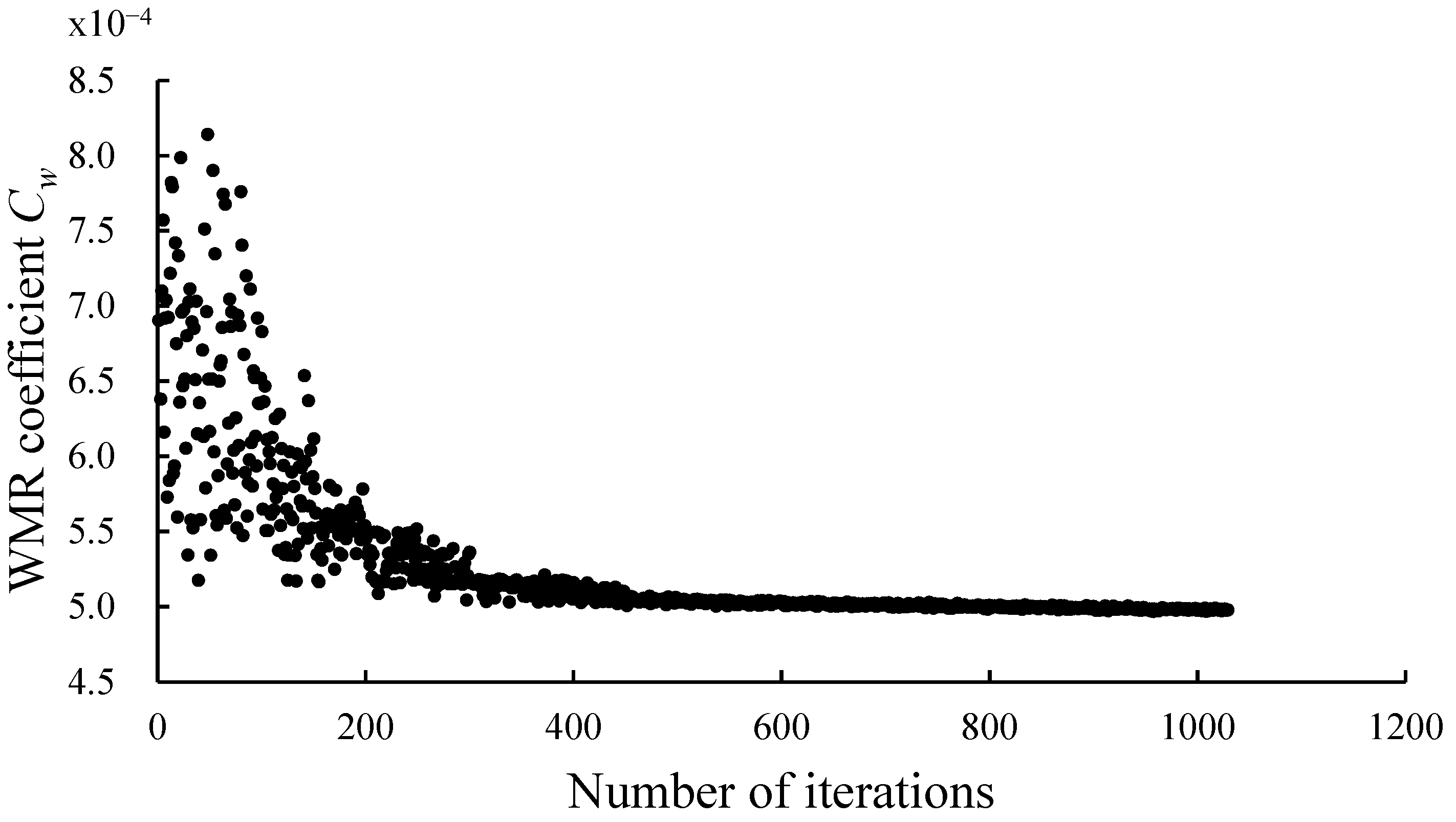
| Number of Iterations for Convergence | WMR Coefficient Cw (Variation %) | WMR Rw (Variation %) | |
|---|---|---|---|
| Original hull form | 6.83 × 10⁻⁴ | 4.647 N | |
| Dimensionality reduction optimization | 1000 | 4.98 × 10⁻⁴ (−27.07%) | 3.394 N (−26.96%) |
| Volume of Displacement
(Variation %) | LCB Lcb (Variation %) | Wetted Surface Area Swet (Variation %) | |
|---|---|---|---|
| Original hull form | 0.550 m3 | 3.293 m | 4.904 m2 |
| Dimensionality reduction optimization | 0.554 m3 (+0.73%) | 3.283 m (−0.30%) | 4.920 m2 (+0.33%) |
| Number of Iterations for Convergence | WMR Coefficient Cw (Variation %) | WMR Rw (Variation %) | Time Consumption of Optimization | |
|---|---|---|---|---|
| Original hull form | 6.83 × 10⁻⁴ | 4.647 N | ||
| Direct optimization | 3000 | 4.98 × 10⁻⁴ (−28.25%) | 3.328 N (−28.38%) | 15 h |
| Dimensionality reduction optimization | 1000 | 4.98 × 10⁻⁴ (−27.07%) | 3.394 N (−26.96%) | 5 h |
| Volume of Displacement
(Variation %) | LCB Lcb (Variation %) | Wetted Surface Area Swet (Variation %) | |
|---|---|---|---|
| Original hull form | 0.550 m3 | 3.293 m | 4.904 m2 |
| Direct optimization | 0.553 m3 (+0.55%) | 3.286 m (−0.21%) | 4.903 m2 (−0.2%) |
| Dimensionality reduction optimization | 0.554 m3 (+0.73%) | 3.283 m (−0.30%) | 4.920 m2 (+0.33%) |
Disclaimer/Publisher’s Note: The statements, opinions and data contained in all publications are solely those of the individual author(s) and contributor(s) and not of MDPI and/or the editor(s). MDPI and/or the editor(s) disclaim responsibility for any injury to people or property resulting from any ideas, methods, instructions or products referred to in the content. |
© 2023 by the authors. Licensee MDPI, Basel, Switzerland. This article is an open access article distributed under the terms and conditions of the Creative Commons Attribution (CC BY) license (https://creativecommons.org/licenses/by/4.0/).
Share and Cite
Chang, H.; Wang, C.; Liu, Z.; Feng, B.; Zhan, C.; Cheng, X. Research on the Karhunen–Loève Transform Method and Its Application to Hull Form Optimization. J. Mar. Sci. Eng. 2023, 11, 230. https://doi.org/10.3390/jmse11010230
Chang H, Wang C, Liu Z, Feng B, Zhan C, Cheng X. Research on the Karhunen–Loève Transform Method and Its Application to Hull Form Optimization. Journal of Marine Science and Engineering. 2023; 11(1):230. https://doi.org/10.3390/jmse11010230
Chicago/Turabian StyleChang, Haichao, Chengjun Wang, Zuyuan Liu, Baiwei Feng, Chengsheng Zhan, and Xide Cheng. 2023. "Research on the Karhunen–Loève Transform Method and Its Application to Hull Form Optimization" Journal of Marine Science and Engineering 11, no. 1: 230. https://doi.org/10.3390/jmse11010230
APA StyleChang, H., Wang, C., Liu, Z., Feng, B., Zhan, C., & Cheng, X. (2023). Research on the Karhunen–Loève Transform Method and Its Application to Hull Form Optimization. Journal of Marine Science and Engineering, 11(1), 230. https://doi.org/10.3390/jmse11010230