Abstract
Formation control, which is a core problem in multi-autonomous underwater vehicle (AUV) systems, plays an important role in realizing safe and accurate cooperation of multi-AUV systems. This paper provides a study on fault-tolerant formation control for multiple stochastic AUV systems under Markovian switching topologies. Considering the effect of noise and Markovian switching communication topology, a novel leader-following group formation control protocol with an actuator fault for a multi-AUV system is developed under the influence of the two independent stochastic processes. The designed controller is proved by an infinitesimal generator with Lyapunov stability theory and can guarantee that the follower AUVs’ states will eventually converge to the leader’s state in each subgroup while forming the desired sub-formation. Finally, the effectiveness of the theoretical analysis is verified by a simulation experiment.
1. Introduction
In recent years, the formation control of multiple autonomous underwater vehicles (AUV) has received considerable attention due to various applications in the field of ocean exploration, deep sea resource development, submarine rescue, trajectory tracking and other fields of ocean engineering. AUV is a kind of self-propelled submersible vehicle that is utilized to perform the desired missions with no human control [1]. Compared with a single AUV, a multi-AUV system can complete the task well in complex applications such as investigating resources, target detection and task accuracy in harsh ocean environments. Further, multi-AUV formation cooperation has more advantages in improving work efficiency and operation scope. The fact that multiple AUVs transmit state information via the sonars in an acoustic channel ensures the coordination of a multi-AUV system. In reality, the AUV system is always affected by stochastic ocean noise. In that case, the multi-AUV system contains uncertain items. In addition, the interaction topology among AUVs may be dynamic or generate new information chains because of the complex marine environments. Stochastic noise and random communication always affect the stability of the multi-AUV system and even lead to the loss of the AUV. Thus, a reliable controller should be designed to guarantee coordination of the multi-AUVs system in the case of noise and random communication. It is still a great challenge because of the highly coupled nonlinearities in the AUV dynamics and the uncertainties in ocean environments.
As the complexity of underwater environment inspection missions increases, formation of multi-AUV can greatly improve the efficiency of exploration and complete more tasks in a limited time. The formation control of a multi-AUV system with a single leader has been investigated in [2,3,4,5,6]. However, in many engineering applications, the strategy with multiple subgroups and leaders of a multi-agent system has stronger practical significance due to the assignment of different geographical locations and tasks [7,8,9]. At the same time, various remarkable results have been dedicated to the formation control problem, and the study made certain progress. The development of formation controllers employs the leader–follower method [10,11,12], consensus method [13,14,15], Lyapunov’s direct method [16,17], model predictive control method [18,19] and back-stepping techniques [20], etc. Among the typical control methods described above, the leader–follower method is widely used in multi-agent formation control because of its good scalability. As a matter of fact, it is a significant theoretical formal method that allows all followers to track the state of leaders. The consensus method is the most basic method in the formation control problem, which is often applied in combination with the leader–follower method.
It is noteworthy that all the studies mentioned above focused on formation control problems with a deterministic switching model manner. In practical applications, the multi-agent systems often suffer from some disturbances, such as communication obstacles under uncertain environments [21,22]. Stochastic switching models could reflect the changes of the information structure, which can be governed by the Markovian switching model. There are many results on multi-agent systems with Markovian switching topologies [23,24,25]. Note that the multi-AUV systems equipped with actuators are at risk of actuator failure in each AUV due to encoding or decoding. Thus far, there have been many studies on the consistency strategy with actuator faults [26,27,28,29].
In the past few years, a rich body of results has been made on formation control for multi-agent systems with stochastic noises. In [30], three formation protocols were established by using a novel stochastic analysis approach for a nonlinear multi-agent systems with communication delays and noise disturbance. Considering the time-varying output and stochastic noise of formation systems, ref. [31] puts forward a fully adaptive practical time-varying output formation protocol. Further, under both measurement and communication noises, ref. [32] designed a robust distributed orientation estimate algorithm and formation control law. Ref. [33] dealt with formation control problems with time delays and multiplicative noises. In [34], a mean-square quasi-composite rotating formation problem with stochastic communication noises was considered by taking coordinate transformation. Up to now, scholars have developed some theories in the research of formation control for stochastic agent systems; however, there are few studies on formation control for multiple stochastic AUV systems with stochastic switching topologies and stochastic noises, which is proposed in our present investigation for the first time.
In previous studies of heterogeneous multi-agent system formation control problems, the heterogeneity dynamics can be divided into two cases: one is that there are different dynamic model equations [35]. For example, the agents’ orders may be first-order, second-order, or high-order in the same system [36,37]; some cross-dimensional formation issues [38], such as the cooperation of an unmanned aerial in three-dimension and surface vehicles in the two-dimensional plane. The other is that each agent has the same dynamic model but different heterogeneous dynamics because of different types, external environment disturbances and configurations of the control objects, as illustrated in [39,40]. Ref. [41] proposed a formation control scheme for multi-AUV systems with heterogenous nonlinear dynamics. Heterogeneous multi-agent systems can be used to solve more practical formation control problems and make the controller have high compatibility and adaptability. In this paper, the leader AUV is equipped with more sensors and constructed as a stable time-invariant system, which can steadily send instructions to the followers. However, the communication topology among all followers is switched randomly. Moreover, the leaders and the followers have different lengths and weights. Under these conditions, the paper focuses on solving the influences of the actuator fault, ocean noise and communication switching on formation control.
Motivated by the above discussions, this paper aims to discuss fault-tolerant formation control for multiple stochastic AUV systems under Markovian switching topologies with multiple leaders. Based on previous research, the contributions of the paper are as follows: (1) the works in [1,3] only considered formation control of a multi-AUV system with a single leader. The paper provides a discussion of the group formation problem in a multi-AUV system with multiple leaders. All the AUVs are divided into multiple subgroups, and each subgroup is controlled to track the average state of the leader while forming the desired sub-formation. (2) The previous research in [42] employed switching communication topologies based on Laplacian matrix theory. In the paper, the fault-tolerant formation control problem is analyzed for the multiple stochastic AUV system with Markov switching topologies, which considers the more random case that two independent stochastic processes exist simultaneously in the system. (3) The communication matrices driven by a Markov process are no longer of Laplacian type, is permitted to be negative in accordance with the group competition and cooperation mechanism. The effect of switching topologies on group formation is determined by the union of topologies of the Markov process, which is more suitable for the limited and unreliable communication topology.
The rest of this paper is arranged as follows: Section 2 introduces some important lemmas, definitions, preliminaries and the AUV model description. Section 3 develops the formation control structure and controller design and presents the main results. Section 4 verifies the effectiveness of the proposed algorithms by simulation. The conclusion is offered in Section 5.
Notations: Table 1 lists some notations and their meanings.

Table 1.
Notations.
2. Preliminaries
This section mainly introduces AUV dynamic models and some related concepts, assumptions and lemmas.
2.1. Problem Formulation
It is well known that the nonlinear characteristics of an AUV are strong when it moves to resist the ocean current in a deep sea with complex terrain. In this paper, the roll velocity of the AUV is ignored due to the fact that the roll motion has less influence on the lateral motion. The AUV is assumed to be under-actuated in the 5-DOF model with the body-fixed and earth-fixed coordination consisting of the surge, sway, heave, pitch and yaw in this paper, which is shown in Figure 1. The dynamic equations of AUV are given as [43].
where the vector denotes the states of the position vector; denotes the states of the velocity vector; the matrix denotes the rotational transformation matrix; M denotes the inertia matrix including the added mass. The paper provides an assumption that the AUV has only a plane symmetry structure. and are the Coriolis and centripetal matrix and the damping matrix; is the vector caused by the effect of gravity and buoyancy; denotes the vector of control input; represents the environmental disturbance forces due to ocean current.
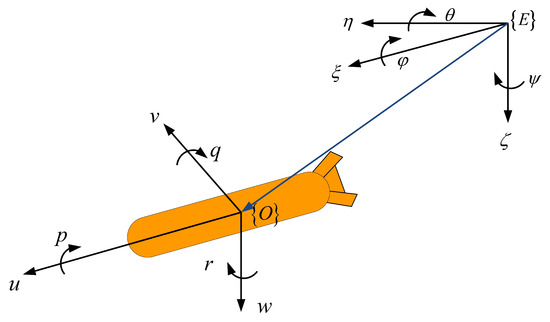
Figure 1.
The coordinate system of the AUV.
In order to simplify the model, assume the AUV has zero buoyancy, and the parameters of the matrices , , and are as follows:
where the details of the above parameters are presented in [43].
Let
the model (1) of the AUV can be represented as [42]:
where
Define the output function . By using the differential manifold theory, the property of the Lie derivative, and relative order [44], we construct the transformation of the new vectors:
Then, the control input and environmental disturbances in the new coordinate system satisfy:
After the coordinate transformation (13) and (14), is used instead of matrix . The dynamical equation of the AUV can be described as follows:
In the transformed coordinate system, the vector of the control input is , and denotes the environmental disturbance forces; therefore, , .
Following the above steps, the control framework of the multi-AUV formation system, which consists of N AUVs, is shown in Figure 2. The control input and the disturbance function of the multi-AUV system in the formation are transformed into the control input and current disturbance function of the original multi-AUV model by inverse coordinate transformation. and are used to satisfy the formation coordination control. The output state of the multi-AUV is used as the control input state of formation control in the new coordinates.
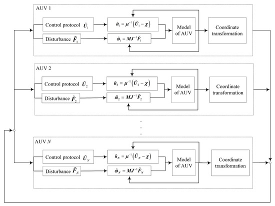
Figure 2.
The formation control scheme of a multi-AUV system.
In AUV system (16), no simplifications are made on system dynamics and disturbances. In this paper, the system (16) is inherently nonlinear and quite consistent with the actual situation, compared with the simplification of the AUV model in [1], which ignores the disturbances.
2.2. Preliminaries
Consider that a multi-AUV system is comprised of N AUVs and M leaders. In the multi-AUV system, the leader has no neighbor. Without loss of generality, we use to denote the AUV set and to denote the leader set. The matrix between the leader and the AUVs is defined by
where if AUV i can receive information from the leader k; otherwise, . It is important to note that an AUV can only follow one leader.
When a multi-AUV formation system performs an ocean survey mission, according to the different locations of the seafloor survey areas and the actual ocean environment, the multi-AUVs may need to arrive at the mission area by different paths, and then the multi-AUV system needs to be divided into several subgroups. In this paper, the multi-AUV system is decomposed into M sub-formations. Each sub-formation contains one leader, and the kth sub-formation contains AUVs. The first AUVs belong to the first sub-formation with the leader ; the AUVs belong to the second sub-formation with the leader ; the rest of the AUVs belong to the last sub-formation with the leader . The number of AUVs in each sub-formation has to satisfy the following equation
Consider the formation control problem for a multiple stochastic AUV system with Markovian switching topologies and multiple leaders based on the AUV dynamical Equation (3), the dynamics of the AUV i are described by
where
is the position state of the ith AUV, and is the velocity state after the coordinate transformation, respectively,
is a continuously differentiable nonlinear function.
The dynamics of the leaders can be described by
where
is a differentiable nonlinear function. is the position state of the jth leader, is the velocity state after the coordinate transformation of the jth leader,
It should be pointed out that the trajectories of the leaders are determined by the actual marine survey mission and the ocean environment, and the motions are assumed to be independent of that of other follower AUVs.
Next, we have the following definition:
Definition 1.
All AUVs in the multiple stochastic AUV system (18) and (19) converge to their respective leader’s trajectory if there exist fixed consensus gains such that for any given initial data and initial distribution of and ,
for , where is the desired constant relative position vector between each AUV i and the leader .
To solve the above formation control problem, we give the following assumptions and lemmas.
Assumption 1.
The union of communication graphs is balanced and contains a directed spanning tree rooting at each leader.
Assumption 2.
For the follower AUV i, the sum of all communication coefficients of the other sub-formations that can exchange information with the AUV i is zero, i.e., , represents the AUV’s neighbor set in the other sub-formations.
The below Lipschitz condition [43,45,46,47,48,49] has been widely used to limit the unknown and bounded nonlinear functions.
Assumption 3.
The nonlinear continuous Lipschitz function is assumed to satisfy the following inequality:
where , is a constant.
Lemma 1
([50]). Let be given matrices such that . Then
if and only if .
Lemma 2
([51]). For M-matrix L, there exists a matrix satisfying , and .
Lemma 3
([52]). Suppose that is measurable and that exists. Then for any ,
Lemma 4
([53]). Consider a stochastic differential equation
where obeys a Markov process, and is the standard Brownian motion, for a positive definite satisfies , the infinitesimal differential generator is defined as
3. Main Results
In the complicated ocean environment, the AUV’s actuator may malfunction. For the ith follower AUV, the actuator fault model is established as follows [27]:
where random variable represents the unknown efficiency control input of the ith AUV with , , . In this paper, we assume that the leader AUV in each sub-formation is fault-free.
Noting that the AUV propulsion system will be affected by the random ocean noise, and the position and velocity state information received by the AUV from its neighbors will be attenuated to a certain extent, it is important to take the impact of noise into account.
Based on the above analysis, the formation control consensus protocol can be designed as
where are gain matrices to be designed, and represent noise intensity, represents the weight of the noise in the information channel of the state variable at time t from the information sending AUV i to the information receiving AUV j,
similarly, denotes the weight of the noise in the information channel of the leader AUV, , . is the measurement noise satisfying
is a one-dimensional Brownian motion defined in total probability space .
The communication topology among agents is described by a randomly switching graph: , which is governed by a Markovian chain with the state space , the transition probability matrix is given by:
where is the transition rate from i to j if , [54].
This paper considers the Markov process ergodic, and the invariant distribution is
for all n possible communication graphs with , respectively, represents the neighbor’s set of the ith AUV. The union communication graph is defined as
and the Laplacian matrix of communication graph is defined as , we have
where is the Laplacian matrix of communication graph . The union of Laplacian matrix is denoted by . The M sub networks of on is denoted by , , and similar notations will be held for .
In this paper, we assume that the stochastic processes and are independent of each other. According to the control protocol (26), the factors affected by noise in underwater acoustic communication are reflected in the form of state measurement error in the control protocol, which is beneficial to the effectiveness analysis of formation control.
Set
where , , , i = 1, …, M in is repeated Ni times, and , i = 1, …, M in is repeated Ni times, is repeated Ni times too.
The system (18) and (19) can be expressed in a structured form as:
where .
Let , , and the system can be written in the following equations associated with the error dynamics:
where , .
Set
The systems (18) and (19) can be recast in the following compact form:
where
By applying the properties of the elementary matrix, the following relationship can be obtained
where
is an elementary matrix.
Lemma 5.
For communication expectation matrix , there exists a matrix satisfying , and .
Proof.
According to literature [55], when is the left eigenvector of associated with eigenvalue , the generalized graph Laplacian potential can be defined as follows
From Assumption 1, it is apparent that
although the matrix does not satisfy the M-matrix condition. Not all in the adjacency matrix are greater than zero when , but according to Assumption 2, for element , which is less than zero, there must exist , in matrix such that ; this yields that
and according to the definition of , we have
thus, we deduce
Our study is motivated by the M-matrix results in [55], where the M-matrix L satisfies Lemma 2. While the result in Lemma 5 is similar to the conclusion based on a non-M matrix, which generalizes the properties of the matrix.
Theorem 1.
Consider the multiple stochastic AUV formation system (32) consisting of M leaders and N followers, the switch topologies are . Under Assumptions 1, 2 and 3, the formation control problem of system (32) can achieve consensus if there exists real matrix P, such that
where , .
Proof.
For and the Markov process , construct the function candidates
then the Lyapunov functional candidate is
Constructing the Lyapunov expectation equation [56]:
By Lemma 4, the infinitesimal differential generator along (32) is given as
where:
and consider:
Let
we can obtain
According to Assumption 3, when satisfies Eq. (21), we have
From Lemma 5 and the properties of , we obtain
From (45), (47), (48) and (49), we obtain
where
According to Lemma 1, it can be concluded that if matrix inequality (40) is achieved, then
In summary, if the conditions in Theorem 1 hold together, the fault-tolerant multiple stochastic AUV system under Markovian switching topologies and multiple leaders attains formation control. The proof is completed.
According to Theorem 1, the design steps for the parameters in the control protocol (26) are as follows:
- Step 1:
- Determine the structure of switching networks and communication topology probability transition.
- Step 2:
- According to Lemma 5, solve matrix by equation .
- Step 3:
- Determine the noise and fault model, and choose the appropriate parameter satisfying .
- Step 4:
- Choose parameters , , calculate parameters , , solve matrix inequality (40), and compute the positive matrix P.
- Step 5:
- Compute the feedback matrices , by equality (46).
In the control protocol (26), is an adjustment parameter. In general, the bigger is, the faster the system (32) converges [57]. The feedback matrices and depend on the union matrix L, which represents the global information of the communication. In [49], a fully distributed protocol was proposed under the directed graph. In the future, we will try to design a controller that only relies on local communication information to realize formation control under switching topology.
After comparison with previous references [11,44,47] on formation control in multi-AUV systems, the innovations of this paper include the following two points. Firstly, this paper studies a multiple stochastic AUV system, considering the general case that the dynamic equations of an AUV include a Brownian motion. Secondly, the topology switching satisfies a stochastic Markov process. Each AUV’s communication topology can be randomly chosen from several preset possible topological graphs according to the probability. Therefore, the paper focuses on the formation control problem where two independent stochastic processes exist in the multi-AUV system. However, there are few studies on the formation control problem of two stochastic processes coexisting in multi-AUV systems in previous literature.
Compared with the existing results [1,3,16] on multi-AUV systems, the group formation and the effects of actuator faults have been considered in this paper. A fault-tolerant control strategy is presented by designing the union communication topology and selecting a Lyapunov expectation equation.
It should be mentioned that the Lyapunov function in Theorem 1 is constructed by taking into account the above two stochastic processes, and the formation control stability is proved by the Lyapunov expectation equation and infinitesimal generator.
4. Simulation
In this section, the numerical example is given to test the effectiveness of the proposed algorithm, and the numerical results are compared with those obtained by the control method proposed in reference [58]. Consider a multi-AUV system with six AUVs and two leaders divided into two sub-formations. The parameters of the leader AUV model are adopted from [59], and the parameters of the follower AUVs model refers to [42]. In addition, we assume that there are 10% uncertainties in the physical parameters of the AUV; that is, the nominal model parameters are reduced by 10% compared to the real parameters. Suppose the constant current is m/s, there are no obstacles in the simulation environment, and the leader AUV in each sub-formation is fault–free.
The initial value of the leader in each sub-formation has been listed in Table 2. The initial locations of the follower AUVs are randomly distributed in the three-dimensional space , and the initial value of velocity is zero. The initial value of pitch angles of the followers AUVs are set in the interval , yaw angles are in the interval , and the simulation time is 2500 s. In order to simulate the motion of AUV more practically, the control input of each AUV is restricted. The thrust amplitude is 1000 N, and the rudder angle amplitude is .
Table 2.
The leaders’ initial value.
The interaction topologies randomly switch between following the Markovian chain with the state space , and the topologies are shown in Figure 3. , and the generator are chosen as
the initial distribution of the Markov process is given by its invariant distribution , and by calculating , it gives
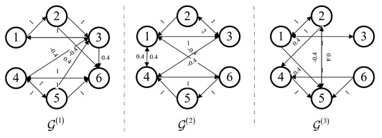
Figure 3.
The network topology graphs.
Consider the nonlinear functions:
Clearly, the function satisfies Assumption 3.
Set
and take
The actuator fault is considered as follows: the actuator of AUV 1 broke down at 1500 s–2500 s with , the actuator of AUV 5 broke down with , and the actuators of other AUVs are normal. In view of Theorem 1, the consensus gains are solved as:
Table 3 shows that the larger the value of parameter , the faster the multiple stochastic AUV system converges, so we select the parameter .
Table 3.
The formation convergence time corresponding to different values of parameter .
The desired paths for the leaders are two helical curves and expressed as:
Figure 4 shows the Markovian states of switching topology. Figure 5 and Figure 6 plot the stochastic noise, which is a Brownian motion , and the distribution is normal. Using the above-mentioned control parameters, Figure 7 presents the position states curves of a multi-AUV system. It can be observed that the follower AUVs 1, 2 and 3 could track the position states of leader 1 and asymptotically approach those of leader 1’s desired path. The follower AUVs 4, 5 and 6 could track the position states of leader 2 and asymptotically approach those of leader 2’s desired path. Figure 8 describes the trajectories of the multi-AUV system with two leaders in three-dimensional space, which shows that the AUV in the same sub-group can reach a consensus with switching topology and stochastic noise through control protocol (26). In Figure 9, one can obtain that the follower AUVs in the same sub-group can form and keep an equilateral triangle formation. In addition, the tracking errors between the leaders and the followers are given in Figure 10 and Figure 11. It can be seen from Figure 10 that the position tracking errors eventually converge to zero after about 500 s. In Figure 11, the velocity tracking error curves oscillate strongly before formation convergence, which is caused by the change in the motion state information. It is generated by the topological switching process, the influence of the external nonlinear disturbance, and the effect of random ocean noise.
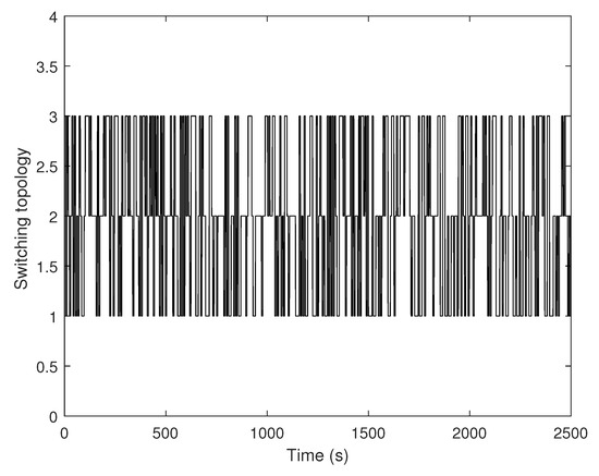
Figure 4.
The Markov states of switching topology.
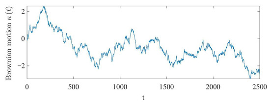
Figure 5.
The Brownian motion .
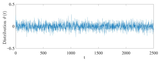
Figure 6.
The distribution of Brownian motion .
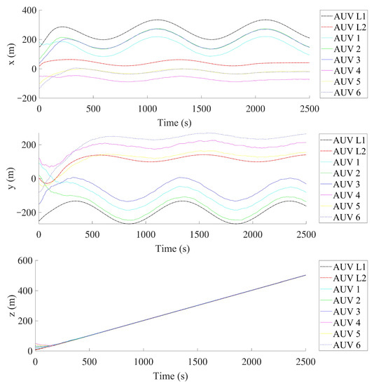
Figure 7.
The position states of a multiple stochastic AUV system.
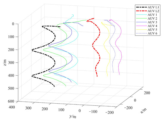
Figure 8.
Three-dimensional trajectories of a multiple stochastic AUV system.
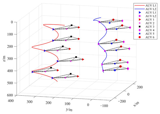
Figure 9.
Position trajectories of a multiple stochastic AUV system.
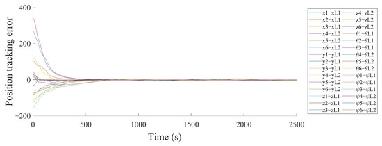
Figure 10.
The position tracking errors of a multiple stochastic AUV system.
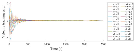
Figure 11.
The velocity tracking errors of a multiple stochastic AUV system.
In the study, we compared the proposed control method with the methods proposed in [58], which studied path tracking control for multi-AUVs considering sampled-data delays and packet losses, to show its effectiveness in dealing with random ocean noise and actuator faults. The sampled-data delays and packet losses are omitted, and the noise and the effect of the actuator fault are added into the path-tracking control method in [58] in order to facilitate the comparison. All other simulation conditions are kept consistent with those in this paper. Figure 12 shows the three-dimensional trajectory of the multi-AUV system. Figure 13 and Figure 14 show the formation errors of follower AUVs. It can be seen that there exist large deviations for the formation position and velocity tracking errors of follower AUVs, which means the leader AUVs of each sub-formation cannot be tracked well by the follower AUVs. Therefore, the above simulation results bring about the conclusion that the proposed control protocols in the paper are valid for multi-AUV system formation control.
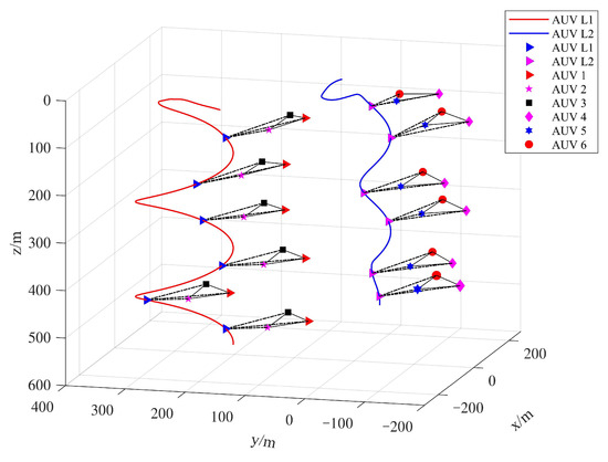
Figure 12.
Position trajectories of a multiple stochastic AUV system in a contrastsimulation.
Figure 13.
The position tracking errors of a multiple stochastic AUV system in a contrast simulation.
Figure 14.
The velocity tracking errors of a multiple stochastic AUV system in a contrast simulation.
5. Conclusions
This paper provides a study on the fault-tolerant formation control problem for a multiple stochastic AUV system with Markovian switching topology. Using the theory of coordinate transformation and differential manifold, the control input and external disturbance of the AUV system are transformed, which is more conducive to the design of the controller and the effectiveness of the formation. In addition, the control protocols with stochastic items and multiple leaders are proposed. The random processes are dominated by the communication Markov process and the Brownian motion of noise, which are independent of each other. The study employed the mathematical expectation function and infinitesimal generator, which contributes to the establishment of some consistent results for the formation control of multiple stochastic AUV systems. Finally, the simulation was performed to verify the effectiveness of the proposed control strategy. Future studies on the formation control for a semi-Markovian jump multiple stochastic AUV system with an event-triggering communication strategy will be conducted.
Author Contributions
Conceptualization, investigation, simulation, writing—original draft, writing—review and editing, X.P.; methodology, funding acquisition, Z.Y.; conceptualization, supervision, methodology, H.J.; investigation, writing-review and editing, methodology, J.Z.; investigation, data curation, L.Y. All authors have read and agreed to the published version of the manuscript.
Funding
This work was partially supported by the National Nature Science Foundation of China under grant No. 52071102, No. 51609048, No. 51909044, Science Foundation for Distinguished Young Scholars of Heilongjiang Province of China under grant No. J2016JQ0052, Harbin Science and Technology Bureau under grant No. 2016RAQXJ080, and Heilongjiang Province Science Foundation for Youths under grant No. QC2017051.
Institutional Review Board Statement
Not applicable.
Informed Consent Statement
Not applicable.
Data Availability Statement
Not applicable.
Conflicts of Interest
The authors declare no conflict of interest.
References
- Zhang, W.; Zeng, J.; Yan, Z.; Wei, S.; Tian, W. Leader-following consensus of discrete-time multi-AUV recovery system with time-varying delay. Ocean Eng. 2021, 219, 108258. [Google Scholar] [CrossRef]
- Li, X.; Zhu, D.Q.; Qian, Y.A. Survey on formation control algorithms for multi-AUV system. Unmanned Syst. 2014, 2, 351–359. [Google Scholar] [CrossRef]
- Gao, Z.Y.; Guo, G. Velocity free leader-follower formation control for autonomous underwater vehicles with line-of-sight range and angle constraints. Inf. Sci. 2019, 486, 359–378. [Google Scholar] [CrossRef]
- Chen, S.; Ho, D.W. Consensus control for multiple AUVs under imperfect information caused by communication faults. Inf. Sci. 2016, 370, 565–577. [Google Scholar] [CrossRef]
- Wang, J.Q.; Wang, C.; Wei, Y.J.; Zhang, C.J. Bounded neural adaptive formation control of multiple underactuated AUVs under uncertain dynamics. ISA Trans. 2020, 105, 111–119. [Google Scholar] [CrossRef] [PubMed]
- Cao, X.; Guo, L.Q. A Leader–follower formation control approach for target hunting by multiple autonomous underwater vehicle in three-dimensional underwater environments. Int. J. Adv. Robot. Syst. 2019, 16, 1729881419870664. [Google Scholar] [CrossRef]
- Han, L.; Xie, Y.; Li, X.D.; Dong, X.W.; Li, Q.D.; Ren, Z. Time-varying group formation tracking control for second-order multi-agent systems with communication delays and multiple leaders. J. Frankl. Inst. 2020, 357, 9761–9780. [Google Scholar] [CrossRef]
- Park, B.S.; Yoo, S.J. Connectivity-maintaining obstacle avoidance approach for leader-follower formation tracking of uncertain multiple nonholonomic mobile robots. Expert Syst. Appl. 2021, 171, 114589. [Google Scholar] [CrossRef]
- Zhang, J.X.; Su, H.S. Time-varying formation for linear multi-agent systems based on sampled data with multiple leaders. Neurocomputing 2016, 339, 59–65. [Google Scholar] [CrossRef]
- Wang, N.; Li, H. Leader–follower formation control of surface vehicles: A fixed-time control approach. ISA Trans. 2022, 124, 356–364. [Google Scholar] [CrossRef]
- Liang, H.; Fu, Y.; Gao, J. Finite-time velocity-observed based adaptive output-feedback trajectory tracking formation control for under actuated unmanned underwater vehicles with prescribed transient performance. Ocean Eng. 2021, 233, 109071. [Google Scholar] [CrossRef]
- Wang, B.; Ashrafiuon, H.; Nersesov, S. Leader–follower formation stabilization and tracking control for heterogeneous planar underactuated vehicle networks. Syst. Control Lett. 2021, 156, 105008. [Google Scholar] [CrossRef]
- Ni, W.; Cheng, D. Leader-following consensus of multi-agent systems under fixed and switching topologies. Syst. Control Lett. 2010, 59, 209–217. [Google Scholar] [CrossRef]
- Du, C.; Bian, Y.; Liu, H.; Ren, W.; Lu, P.; Liu, X. Cooperative startup control for heterogeneous vehicle platoons: A finite-time output tracking-based approach. IEEE Trans. Control Netw. 2021, 8, 1767–1777. [Google Scholar] [CrossRef]
- Griparic, K.; Polic, M.; Krizmancic, M.; Bogdan, S. Consensus-Based Distributed Connectivity Control in Multi-Agent Systems. IEEE Trans. Netw. Sci. Eng. 2022, 9, 1264–1281. [Google Scholar] [CrossRef]
- Thanh, P.N.; Tam, P.M.; Anh, H.P. New approach for three-dimensional trajectory tracking control of under-actuated AUVs with model uncertainties. Ocean Eng. 2021, 228, 108951. [Google Scholar] [CrossRef]
- Karkoub, M.; Wu, H.M.; Wang, H. Nonlinear trajectory-tracking control of an autonomous underwater vehicle. Ocean Eng. 2017, 145, 188–198. [Google Scholar] [CrossRef]
- Shen, C.; Shi, Y. Distributed implementation of nonlinear model predictive control for AUV trajectory tracking. Automatica 2020, 115, 108863. [Google Scholar] [CrossRef]
- Yan, Z.; Gong, P.; Zhang, W.; Wu, W. Model predictive control of autonomous underwater vehicles for trajectory tracking with external disturbances. Ocean Eng. 2020, 217, 107884. [Google Scholar] [CrossRef]
- Cho, G.R.; Li, J.H.; Park, D.; Jung, J.H. Robust trajectory tracking of autonomous underwater vehicles using back-stepping control and time delay estimation. Ocean Eng. 2020, 201, 107131. [Google Scholar] [CrossRef]
- Yang, S.; Bai, W.W.; Li, T.S.; Shi, Q.; Yang, Y.; Wu, Y.; Chen, C.P. Neural-network-based formation control with collision, obstacle avoidance and connectivity maintenance for a class of second-order nonlinear multi-agent systems. Neurocomputing 2021, 439, 243–255. [Google Scholar] [CrossRef]
- Zhang, J.X.; Su, H.S. Formation-containment control for multi-agent systems with sampled data and time delays. Neurocomputing 2019, 424, 125–131. [Google Scholar] [CrossRef]
- He, M.H.; Mu, J.R.; Mu, X.W. Leader-following consensus of nonlinear multi-agent systems under semi-Markovian switching topologies with partially unknown transition rates. Inf. Sci. 2020, 513, 168–179. [Google Scholar] [CrossRef]
- Gao, J.F.; Li, J.H.; Pan, H.P.; Wu, Z.G.; Yin, X.X.; Wang, H.J. Consensus via event-triggered strategy of nonlinear multi-agent systems with Markovian switching topologies. ISA Trans. 2020, 104, 122–129. [Google Scholar] [CrossRef] [PubMed]
- Ma, T.D.; Li, K.; Zhang, Z.L.; Cui, B. Impulsive consensus of one-sided Lipschitz nonlinear multi-agent systems with Semi-Markov switching topologies. Nonlinear Anal. Hybrid Syst. 2021, 40, 101021. [Google Scholar] [CrossRef]
- Wan, L.; Cao, Y.; Sun, Y.C.; Qin, H. Fault-tolerant trajectory tracking control for unmanned surface vehicle with actuator faults based on a fast fixed-time system. ISA Trans. 2022, 130, 79–91. [Google Scholar] [CrossRef] [PubMed]
- Cao, Y.; Li, B.; Wen, S.; Huang, T. Consensus tracking of stochastic multi-agent system with actuator faults and switching topologies. Inf. Sci. 2022, 607, 921–930. [Google Scholar] [CrossRef]
- Sun, Y.; Shi, P.; Lin, C. Adaptive consensus control for output-constrained nonlinear multi-agent systems with actuator faults. J. Frankl. Inst. 2022, 359, 4216–4232. [Google Scholar] [CrossRef]
- Lu, Y.; Xu, X.; Qiao, L.; Zhang, W. Robust adaptive formation tracking of autonomous surface vehicles with guaranteed performance and actuator faults. Ocean Eng. 2021, 237, 109592. [Google Scholar] [CrossRef]
- Lai, J.; Chen, S.; Lu, X.; Zhou, H. Formation tracking for nonlinear multi-agent systems with delays and noise disturbance. Asian J. Control 2015, 17, 879–891. [Google Scholar] [CrossRef]
- Yu, J.; Dong, X.; Li, Q.; Lü, J.; Ren, Z. Fully adaptive practical time-varying output formation tracking for high-order nonlinear stochastic multiagent system with multiple leaders. IEEE Trans. Cybern. 2019, 51, 2265–2277. [Google Scholar] [CrossRef] [PubMed]
- Wang, B.; Tian, Y. Distributed formation control: Asymptotic stabilization results under local noisy information. IEEE Trans. Cybern. 2019, 51, 16–27. [Google Scholar] [CrossRef] [PubMed]
- Jia, R.; Zong, X. Time-varying formation control of linear multiagent systems with time delays and multiplicative noises. Int. J. Robust Nonlin. 2021, 31, 9008–9025. [Google Scholar] [CrossRef]
- Mo, L.; Yuan, X.; Jia, Y.; Guo, S. Mean-square Quasi-composite Rotating Formation Control of Second-order Multi-agent Systems under Stochastic Communication Noises. J. Robot. Netw. Artif. Life 2019, 6, 89–96. [Google Scholar] [CrossRef]
- Wang, N.; Ahn, C. Coordinated trajectory-tracking control of a marine aerial-surface heterogeneous system. IEEE/ASME T. Mech. 2021, 26, 3198–3210. [Google Scholar] [CrossRef]
- Long, J.; Wang, W.; Wen, C.; Huang, J.; Lü, J. Output feedback based adaptive consensus tracking for uncertain heterogeneous multi-agent systems with event-triggered communication. Automatica 2020, 136, 110049. [Google Scholar] [CrossRef]
- Shimin, W.; Zhi, Z.; Zhong, R.; Wu, Y.; Peng, Z. Adaptive distributed observer design for containment control of heterogeneous discrete-time swarm systems. Chin. J. Aeronaut. 2020, 33, 2898–2906. [Google Scholar]
- Wang, S.; Zhan, Z.; Zhong, R.; Wu, Y.; Peng, Z. Cross-dimensional formation control of second-order heterogeneous multi-agent systems. ISA Trans. 2022, 127, 188–196. [Google Scholar]
- Hu, W.; Liu, L. Cooperative output regulation of heterogeneous linear multi-agent systems by event-triggered control. IEEE Trans. Cybern. 2016, 47, 105–116. [Google Scholar] [CrossRef]
- Liu, H.; Peng, F.; Modares, H.; Kiumarsi, B. Heterogeneous formation control of multiple rotorcrafts with unknown dynamics by reinforcement learning. Inf. Sci. 2021, 558, 194–207. [Google Scholar] [CrossRef]
- Yuan, C.; Licht, S.; He, H. Formation learning control of multiple autonomous underwater vehicles with heterogeneous nonlinear uncertain dynamics. IEEE Trans. Cybern. 2017, 48, 2920–2934. [Google Scholar] [CrossRef] [PubMed]
- Yan, Z.P.; Yang, Z.W.; Yue, L.D.; Wang, L.; Jia, H.M.; Zhou, J.J. Discrete-time coordinated control of leader-following multiple AUVs under switching topologies and communication delays. Ocean Eng. 2019, 172, 361–372. [Google Scholar] [CrossRef]
- Fossen, T.I. Handbook of Marine Craft Hydrodynamics and Motion Control; John Wiley & Sons: Trondheim, Norway, 2011; pp. 81–89. [Google Scholar]
- Lin, X.; Tian, W.; Zhang, Y.; Li, Z.; Zhang, C. The fault-tolerant consensus strategy for leaderless Multi-AUV system on heterogeneous condensation topology. Ocean Eng. 2022, 245, 110541. [Google Scholar] [CrossRef]
- Yu, W.; Ren, W.; Zheng, W.; Chen, G.; Lü, J. Distributed control gains design for consensus in multi-agent systems with second-order nonlinear dynamics. Automatica 2013, 49, 2107–2115. [Google Scholar] [CrossRef]
- Li, Z.; Ren, W.; Liu, X.; Fu, M. Consensus of multi-agent systems with general linear and Lipschitz nonlinear dynamics using distributed adaptive protocols. IEEE Trans. Automat. Contr. 2012, 58, 1786–1791. [Google Scholar] [CrossRef]
- Yan, Z.; Zhang, M.; Zhang, C.; Zeng, J. Decentralized formation trajectory tracking control of multi-AUV system with actuator saturation. Ocean Eng. 2022, 255, 111423. [Google Scholar] [CrossRef]
- Sader, M.; Chen, Z.; Liu, Z.; Deng, C. Distributed robust fault-tolerant consensus control for a class of nonlinear multi-agent systems with intermittent communications. Appl. Math. Comput. 2021, 403, 126166. [Google Scholar] [CrossRef]
- Li, X.; Wang, J. Fault-tolerant tracking control for a class of nonlinear multi-agent systems. Syst. Control Lett. 2020, 135, 104576. [Google Scholar] [CrossRef]
- Fossen, T.I. Linear Matrix Inequalities in System and Control Theory; SIAM: Philadelphia, PA, USA, 1994; pp. 56–121. [Google Scholar]
- Meng, M.; Liu, L.; Feng, G. Adaptive output regulation of heterogeneous multiagent systems under Markovian switching topologies. IEEE Trans. Cybern. 2017, 48, 2962–2971. [Google Scholar] [CrossRef]
- Fragoso, M.D.; Costa, O.L.V. A unified approach for stochastic and mean square stability of continuous-time linear systems with Markovian jumping parameters and additive disturbances. SIAM J. Control Optim. 2005, 44, 1165–1191. [Google Scholar] [CrossRef]
- Li, K.; Mu, X. Containment control of stochastic multiagent systems with semi-Markovian switching topologies. Int. J. Robust Nonlin. 2019, 29, 4943–4955. [Google Scholar] [CrossRef]
- Meyn, S.P.; Tweedie, R.L. Markov Chains and Stochastic Stability; Springer Science & Business Media: Cambridge, UK, 2012; pp. 48–72. [Google Scholar]
- Zhang, H.; Lewis, F.; Qu, Z. Lyapunov, adaptive, and optimal design techniques for cooperative systems on directed communication graphs. IEEE Trans. Ind. Electron. 2011, 59, 3026–3041. [Google Scholar] [CrossRef]
- Wang, H.; Xue, B.; Xu, A. Leader-following consensus control for semi-Markov jump multi-agent systems: An adaptive event-triggered scheme. J. Frankl. Inst. 2021, 358, 428–447. [Google Scholar] [CrossRef]
- Ren, W.; Beard, R.W. Distributed Consensus in Multi-Vehicle Cooperative Control; Springer: London, UK, 2008; pp. 25–40. [Google Scholar]
- Yan, Z.; Yang, Z.; Pan, X.; Zhou, J.; Wu, D. Virtual leader based path tracking control for Multi-UUV considering sampled-data delays and packet losses. Ocean Eng. 2020, 216, 108065. [Google Scholar] [CrossRef]
- Yan, Z.; Yu, H.; Li, B. Bottom-following control for an underactuated unmanned undersea vehicle using integral-terminal sliding mode control. J. Cent. South Univ. 2011, 22, 4193–4204. [Google Scholar] [CrossRef]
Disclaimer/Publisher’s Note: The statements, opinions and data contained in all publications are solely those of the individual author(s) and contributor(s) and not of MDPI and/or the editor(s). MDPI and/or the editor(s) disclaim responsibility for any injury to people or property resulting from any ideas, methods, instructions or products referred to in the content. |
© 2023 by the authors. Licensee MDPI, Basel, Switzerland. This article is an open access article distributed under the terms and conditions of the Creative Commons Attribution (CC BY) license (https://creativecommons.org/licenses/by/4.0/).