Article

An Improved Bald Eagle Search Algorithm for Global Path Planning of Unmanned Vessel in Complicated Waterways

1
Airport College, Binzhou University, Binzhou 256600, China
2
Navigation College, Dlian Maritime University, Dalian 116026, China
3
National Engineering Research Center for Water Transport Safety, Wuhan 430063, China
*
Author to whom correspondence should be addressed.
J. Mar. Sci. Eng. 2023, 11(1), 118; https://doi.org/10.3390/jmse11010118
Submission received: 18 November 2022 / Revised: 15 December 2022 / Accepted: 24 December 2022 / Published: 5 January 2023
(This article belongs to the Special Issue Ship Collision Risk Assessment)

Abstract

:
The path planning of unmanned ships in complex waters using heuristics usually suffers from problems such as being prone to fall into the local optimum, slow convergence, and instability in global path planning. Given this, this paper proposes a Self-Adaptive Hybrid Bald Eagle Search (SAHBES) Algorithm by incorporating adaptive factors into the traditional BES in order to enhance the early global searching ability of the BES algorithm. Moreover, Pigeon-Inspired Optimization (PIO) is introduced to overcome the disadvantage of traditional BES algorithms: that it is easy for them to fall into local optimization. This study improves the fitness function by adding a distance between the ships’ path corners. The obstacle is based on the calculation of the path length. The curve optimization module is applied to smooth the obtained path to generate more rational path planning results, which means the path is the shortest and avoids collision successfully. A simulation test of the SAHBES algorithm on the path planning under different obstacle scenarios is conducted by using the MATLAB platform. The results show that SAHBES can generate the shortest safe, smooth path in different complex water environments, considering the limitations of fundamental ship maneuvering operations compared to other algorithms, thus verifying the feasibility and efficiency of the proposed SAHBES algorithm.

1. Introduction

In recent years, with the development of water transportation, the number of ships has increased dramatically, and the size of the vessels has mainly expanded. Suppose ship collision accidents occur in the navigation area. In that case, the navigation of ships near the accident area will be affected, and the leakage accident caused by the collision will cause large-scale pollution in the water area. Therefore, effectively reducing the risk of ship collision is a significant challenge facing the current shipping safety field [1].
The research on ship collision avoidance systems is significant to ship navigation safety.
The path planning of ships is more complex than that of mobile robots due to the influence of factors such as the navigation environment and ship maneuverability. Therefore, autonomous collision avoidance, path planning, and other issues of unmanned ships have always been the research focus of the shipping industry. Ship path planning methods can be broadly grouped into two categories. One is deterministic ship path planning based on mathematical, physical, and other theoretical backgrounds; the other is based on intelligent optimization techniques, such as a heuristic algorithm.

1.1. Complicated Waters

At present, there is no clear definition of complex waters, which usually refers to waters with poor natural conditions, complex ship traffic flow, and great difficulty for ships to navigate, including offshore construction waters, bridge area waters, multi-channel intersection waters, channel bending sections, narrow channel sections, shoal navigation areas, and the dam area navigation section, anchoring area, fishing area for fishing vessels, island and reef area [2].
However, the complex waters studied in this paper mainly include waters with a high navigation density and many obstacles, which make it challenging to avoid ship collisions.

1.2. Ship Collision Avoidance Path Planning Based on Deterministic Mathematical Methods

The research on ship collision avoidance based on deterministic methods such as mathematics and physics primarily uses geometry, analytics, kinematics, and field theory. The research history can trace back to the early 1990s. The Japanese scholars Iijima and Hagiwara [3] developed a ship-automatic collision avoidance decision control system that automatically implements collision avoidance strategies. This control system uses the breadth-first search method to select and plan collision avoidance paths. However, in thedesign of the system, the single collision avoidance scenario lacks universality.
With the rapid development of the shipping industry, ship collision avoidance has become a hot issue in maritime transportation. More and more, scholars have invested in ship collision avoidance and path planning. Tsou et al. [4] used the predicted area of danger (PAD) theory in the principle of ship collision avoidance. The relative speed, the relative orientation of two ships, and the distance to the closest point of approach (DCPA) or time of closest point of approach (TCPA) predict the area where other ships may collide with their ship in the future and regard the PAD area as a static obstacle. The evolutionary algorithm searches for a safe path to avoid static obstacles and PAD areas. Zhang et al. [5] proposed a real-time collision avoidance method for under-actuated ships based on improved dynamic virtual ships, which uses a control method combining neural networks and robust neural damping technology to achieve automatic collision avoidance. During collision avoidance, the course angle and speed change smoothly, which is consistent with the actual navigation of ships. Jeong et al. [6] proposed a multi-criteria path planning technique to quantitatively assess the navigation traffic risk of routes using ship domain models, and then by structuring the data into contour maps. Finally, the path planning model is established based on the main criteria of security and efficiency. The AIS data from the numerical simulation and actual evaluation show that the technology can generate and evaluate target-oriented routes at the same time. Huang et al. [7] proposed a generalized velocity obstacle algorithm (GVO) for ship path planning. This algorithm effectively compensates for the shortcomings of previous collision avoidance path planning research by assuming a constant speed, ignoring the ship kinematics model, and not taking the Convention on the International Regulations for Preventing Collisions at Sea (COLREG) into account. Yu et al. [8] proposed a path planning method based on dynamic cluster analysis (DCA) because of the long iteration time of path planning in the situation of multi-ship encounters and the impact of target ship behavior changes on path planning. This method reduced the number of calculation targets and improved the efficiency of path planning. Chen et al. [9] proposed a hybrid method for global path planning of marine autonomous surface ships (MASS), which used the concept of time-varying collision risk (TCR) to calculate the collision risk between ships and obstacles. Moreover, the team also proposed a new cost function to combine the proximity of obstacles with the impact of collision risk in the region; finally, the fast-marching square algorithm is used to generate the globally optimal path. Zhao et al. [10] first proposed a path-tracking control algorithm for surface ships based on global heading constraints. The controller is designed using a closed-loop gain-shaping algorithm (CGSA) and nonlinear feedback technology. The algorithm ensures that the ship can follow the predetermined track with a slight rudder angle, rolling angle, and smooth course change, to be more in line with other maritime transportation.

1.3. Ship Collision Avoidance Path Planning Based on Heuristic Algorithms

With the rapid development of artificial intelligence, heuristic algorithms such as the A star algorithm, deep reinforcement learning [11,12], the particle swarm optimization algorithm, the genetic algorithm [13], and Markov decision making have also been extensively applied in collision avoidance decision-making and path planning.
Singh [14] proposed the use of the A star method for the current and dynamic and static obstacles in the marine environment, as it is used to plan the optimal path of unmanned ships in a restricted marine environment. The simulation of different environmental conditions proves that this method can generate a safer route path without reducing navigation efficiency based on the traditional A star. He et al. [15] proposed a dynamic path planning method based on the A star algorithm and ship navigation rules for complex multi-ship encounter situations, namely, the Dynamic Anti-collision A-Star (DAA star) algorithm. This algorithm considers the maneuverability constraints of a single ship and the differences between ships, and can solve the path planning problem of dynamic obstacles in multi-ship encounter situations. Xie et al. [16] proposed a global and multi-directional A-star algorithm, which first displayed the artificial potential field (APF) in a scalar mode.
Furthermore, a punishment mode was established for submarine pipelines, which, combined with the A star optimization algorithm, reasonably planned out the path of working ships in the offshore wind farm to ensure the safety and efficiency of navigation. Tharwat et al. [17] used the model of the Bezier curve to plan the path, used a new chaotic particle swarm optimization algorithm to optimize the control points of the Bezier curve, and proposed two variants of particle swarm optimization algorithm: CPSO-I and CPSO-II. The experiment proved that both variants could find the optimal path. Based on the premise that there is no external interference in the open sea area, Li et al. [18] used the improved multi-objective optimization algorithm NSGA-II, combined with the ship domain model, to conduct collision avoidance simulation experiments. The experimental results show that this method can optimize the ship’s collision avoidance strategy and provide a reasonable scheme for the ship’s navigation path. Joohyun and Nakwan [19] proposed an autonomous collision avoidance method based on deep reinforcement learning for the collision avoidance process of unmanned surface ships. This method uses the visual recognition ability of the deep neural network to analyze the encounter situation of ships and determine the stand-on and giveaway vessels. The deep learning, combined with the Markov decision-making model, is used to establish a collision avoidance simulation experiment, and the optimal collision avoidance strategy is obtained through continuous iterative training. Xue [20] designed a sine-cosine particle swarm optimization (SC-PSO) algorithm based on quasi-reflection. The new algorithm has a fast convergence speed and ideal results, and the effectiveness and rationality of the algorithm have been proven through simulation experiments. Han et al. [21] proposed a dynamic hybrid path planning scheme. In this method, a non-uniform cost map with a risk function for global path planning and an implemented reverse search from the target node through a non-uniform Theta-A star are used to solve the problem of a path falling into the local optimum. Experimental results show the effectiveness of the proposed algorithm.
In conclusion, the ship collision avoidance model based on the deterministic mathematical method has high computational complexity and accurate results. However, such methods generally only consider the navigation status between collision avoidance ships for calculation and often need to consider the changeable and complex navigation environment at sea, with a poor degree of freedom and generalization ability. In order to solve this problem, artificial intelligence algorithms are widely used in ship collision avoidance and path planning. With the help of computers, vessels’ collision avoidance simulation experiments can consider the impact of ship parameters, the external environment, and other complex factors on collision avoidance between ships, making the collision avoidance process more realistic and the results more accurate. However, most heuristic algorithms require extensive training and many iterations to get accurate results, which sometimes affects computational efficiency. In order to solve this problem, this paper refers to the idea of the Bald Eagle Search Algorithm. It proposes an adaptive hybrid eagle Search Algorithm to study ship collision avoidance and path planning.
In order to solve the problems of global path planning for unmanned ships in complex waters, which ca easily fall into the local optimum with slow and unstable convergence, this paper is inspired by the Bald Eagle Search Algorithm (BES). It makes various improvements based on the traditional BES: firstly, the adaptive control factor is introduced in the structure of the algorithm, and some ideas of the pigeon flock algorithm are incorporated; secondly, the structure of the fitness function is combined with the structure of the adaptive degree function which is combined with the actual navigation and curve optimization module to make corresponding improvements. The proposed model converges faster and iterates more efficiently, which means it has robustness and does not easily fall into the local optimum.
The rest of the paper is constructed as follows: the Section 2 introduces the improvement of the traditional BES algorithm and the calculation process of the proposed collision avoidance algorithm in detail and selects four groups of test functions to verify the feasibility of the adaptive hybrid BES algorithm. In Section 3, four groups of obstacle avoidance experiments are designed and compared with the adaptive particle swarm optimization algorithm and the traditional BES algorithm. Section 4 concludes this research.

2. Methodology

The BES algorithm was first proposed by Malaysian scholar Alsattar [22] in 2020. It is a meta-heuristic algorithm based on the predation process of the bald eagle. It simulates the bald eagle’s hunting strategy or intelligent social behavior when searching for prey. In this paper, it is equivalent to the behavior of finding the optimal path. BES hunting is divided into three stages: the first stage is to select the space with the most prey, the second stage is to search for prey in the selected space, and the third stage is to conduct diving hunting. The whole algorithm will repeat these three stages in each iteration. The mathematical expression of the three stages of the traditional BES is shown as follows.
(1) Selection stage:
The individual determines the search space through the optimal fitness to the initial population and the average position of the current population and randomly selects the direction to update the individual post to a new area near the previous search area to continue to choose. The particular location update method is shown in Equation (1):
P n e w , i = P b e s t + α ε ( P m e a n P i )
where α = [1.5, 2] refers to factors controlling position changes, ε is a uniform random number in [0, 1], Pbest is the current optimal individual position, Pi is the position at this moment, and Pmean is the average position of the population.
(2) Prey searching stage:
In the prey-searching stage, the eagles will update their positions with the trajectory of Archimedes’s spiral around the current status. The formulas are shown as follows:
P n e w , i = P i + x i ( P i P m e a n ) + y i ( P i P i + 1 )
where x i ,   y i ;   x r i ,   y r i ;   θ i ,   r i can be respectively expressed by Equations (3)–(5):
{ x i = x r i max ( | x r | ) y i = y r i max ( | y r | )
{ x r i = r i × cos ( θ i ) y r i = r i × sin ( θ i )
{ θ i = α i × π × ε r i = θ i × R × ε
In Equation (5), α [ 5 ,   10 ] , R [ 0.5 ,   2 ] , which is the parameter that controls the spiral path, θi and r i are the polar angle and polar diameter of the spiral equation, and x i and y i are the positions of corresponding individuals in Cartesian coordinates. The value is [ 1 ,   1 ] to change the spiral shape.
It can be seen that an individual flies around himself, and the flying distance is determined by the distance between himself and the center of the group and the distance between himself and the following individual (if the current individual is the last in the group, its following individual is the first individual in the group).
(3) Swooping stage:
In the swooping stage, the population dives from the best position in the search space to the target. The specific formula is shown as follows:
P n e w , i = ε P b e s t + x i ( P i c 1 P m e a n ) + y i ( P i c 2 P b e s t )
{ x i = x r i max ( | x r | ) y i = y r i max ( | y r | )
{ x r i = r i × cos h ( θ i ) y r i = r i × sin h ( θ i )
{ θ i = α × π × ε r i = θ i
where c1 and c2 refer to a constant number and the general value range is [1, 2]. In this stage, individuals will update their positions around the optimal individuals in a spiral path. In the position update process in the swoop stage, the optimal individual position is a random coefficient. The parameters c1 and c2 will increase the movement intensity of the individual toward the best point and the center point. The algorithm will accelerate the convergence speed at the beginning if there is no random coefficient. However, when it is near the best point, it will produce oscillation, resulting in no convergence. The other three stages have a common step: if the new position obtained by searching is better than the original one, the individual will update to the new one. Otherwise, it will stay in its original position. Because of the special structure of the traditional BES algorithm, it calculates the fitness three times in each population update process. Combined with the search path of Archimedes spiral, the algorithm converges very quickly in the early iteration, making it easy for it to fall into the local optimum. The process of the traditional BES algorithm is shown in Figure 1.
In addition, the location update method in the traditional BES at each stage also has some improvement: in the region selection stage, from Equation (1), it can be seen that the search performance in this stage mainly depends on the value of control factor. Control factor α is a fixed value, and the optimization potential of the algorithm cannot be fully exerted. In the swoop phase, from Equation (6), it can be seen that, because there is a random coefficient of [0, 1] before the optimal position, its position will gradually converge to 0; when the optimal solution is not at 0, the result is relatively poor. Aiming at the above shortcomings and considering the unique requirements of path planning in the unmanned ship, this paper proposes two improvement strategies for the traditional BES.

2.1. Algorithm Structure Improvement

In order to maximize the optimization potential of the algorithm, this paper introduces an adaptive control factor to determine the value of the control factor in the selection region stage. The adaptive control factor can adjust its value with the increasing number of iterations so that the individuals in the early iteration of the algorithm fly away from the population to increase population diversity, expand the search range, and maintain good global search performance. In contrast, in the late iteration, they gather in the optimal global direction, making the algorithm cluster, thus enhancing the local optimization ability of the algorithm and accelerating the convergence speed. This paper designs an adaptive control factor whose value decreases with the number of iterations α . The improved mathematical expression of α is shown as follows:
α = α max ( α max α min ) × ( t T ) 2
where αmax and αmin respectively represent the maximum and minimum values of α in traditional BES, t refers to the number of iterations of the current algorithm, and T represents the maximum number of iterations of the algorithm.
On the other hand, to improve the algorithm’s zero tendencies, this paper adds part of the idea of the pigeon swarm algorithm in the dive phase of the traditional BES. First, it needs to sort the individuals of the population according to the corresponding fitness function value and divide the population into two groups. The better group keeps its position unchanged while providing its average position as a parameter. At the same time, α is used to adaptively adjust the new position determined by the group with poor fitness to enrich the diversity of the population while preserving the population advantage. If the fitness value of the individual position after the grouping update is better than that of the original individual, the new individual is retained. Otherwise, the original is maintained. The specific formulas are shown as follows:
{ P m e a n = i i N ( P i × f ( P i ) ) N × i = 1 N f ( P i ) N = N 2
{ P n e w , i = P i + α × ( P m e a n P i ) , f ( P n e w , i ) < f ( P i ) P n e w , i = P i , f ( P n e w , i ) f ( P i )
where N refers to the total number of individuals in the eagle population, and Equation (11) gives the average position of the better part of individuals. At the same time, Equation (12) shows that the worse part of individuals randomly flies a distance toward the center of gravity of the better part of individuals.
In order to verify whether the algorithm improvement is reasonable, this paper selects four groups of functions for the maximum value search test. Because the global path planning of ships has the characteristics of high demand population dimension and a large number of locally optimal solutions, the optimal solution is not fixed. This paper selects 4 multimodal surface functions from 23 standard test functions and makes minor changes to them before the test; the optimal value deviates from the (0,0) point. At the same time, it is complicated to a certain extent, increasing the difficulty of optimization. The four test function names, the dimensions of the test population, and the search range are shown in Table 1.
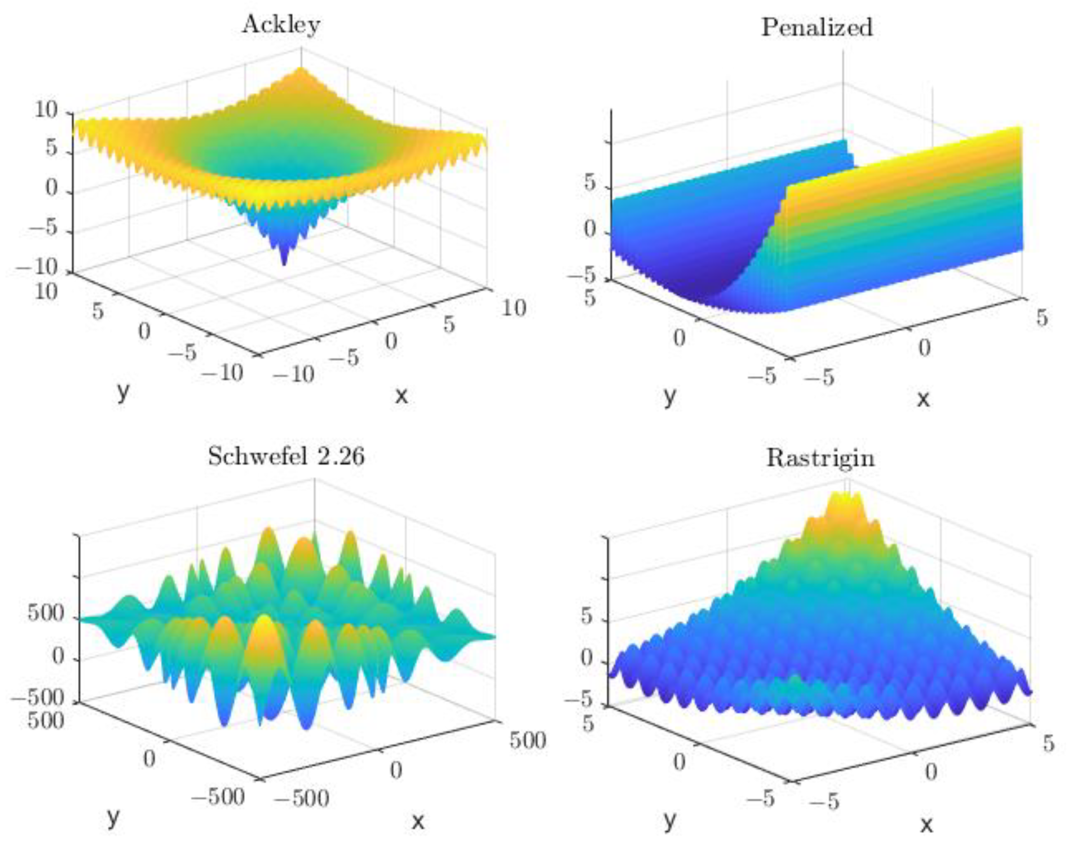
Compared with the function prototype, the minimum value of the function and the position coordinates corresponding to the minimum value are the main differences. The modified function image is shown in Figure 2.
As shown in Figure 2, the characteristic of the Ackley function is that it has a large number of local minima but only one global minimum, which brings the risk that optimization algorithms, especially mountain climbing algorithms, are trapped in one of their many local minima. The distribution of Schwefel 2.26 function values is exceptionally irregular. Similarly to Ackley, there are a large number of local minima and only one global minimum. In addition, the Penalized function is similar to the Rastigin function, although the function image is quite different, and there are also many local minima. They are highly multimodal, but the minimum values are regularly distributed.
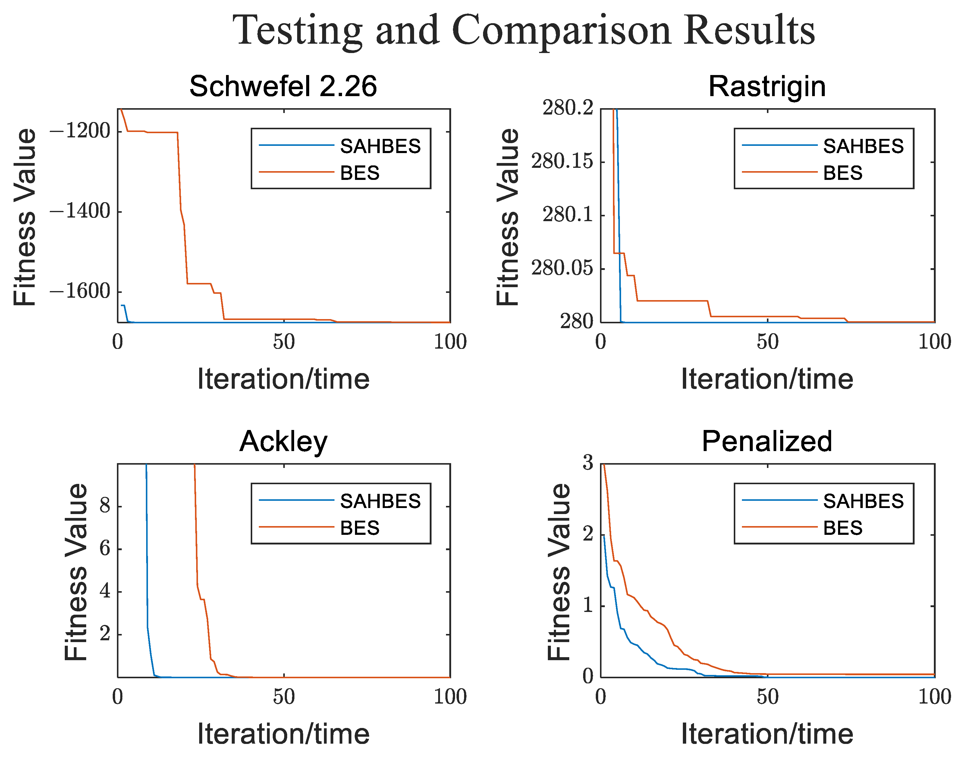
Assume that the number of the eagle is 50, the number of iterations is 100, and the population dimension is uniformly set to 30. The size of the current optimal value reached by the population after the iteration or the number of iterations reaching the optimal global value is taken as the basis for evaluating the optimization effect of the algorithm. At the same time, in order to test the robustness of the algorithm, this paper runs each test function 50 times with the traditional BES and SAHBES algorithms and averages the fitness curve to get the final result, as shown in Figure 2.
It can be seen from Figure 3 that the improved BES algorithm performs well in the test results of the four functions, and its convergence speed is more robust than that of the traditional BES algorithm. In the four groups of tests, SAHBES can reach the optimal value of the function after an average of 15 iterations, while the traditional BES requires an average of 65 iterations. In terms of convergence efficiency, SAHBES is 77% higher than the traditional BES. In the test results of F1 and F2 functions, the optimization effect of SAHBES not only makes it fast in convergence but also more potent than that of traditional BES when it falls into local optimization. From the above, the overall performance of SAHBES is better than that of traditional BES.

2.2. Improvement of Fitness Function

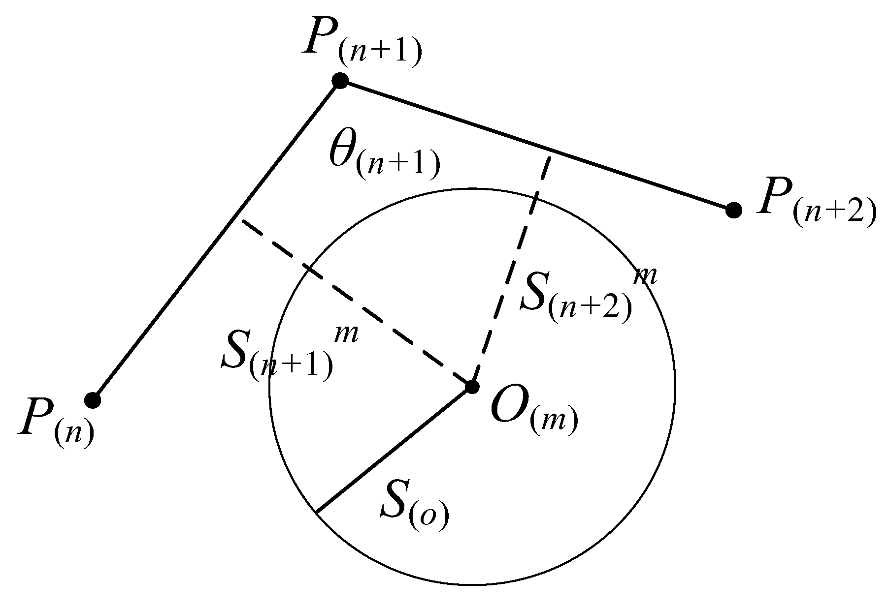
The general global path planning method only aims at finding the shortest path, but many factors must be considered in the actual waters. Considering the limitations of the self-maneuverability of the unmanned ship when traveling and the requirements for navigation safety, this paper adds the turning angle function and the safety distance function to the path length function when calculating the fitness function. The overall fitness function of the path is obtained by weighted average processing of the three functions, to obtain the safest path that meets the maneuverability of the ship. To facilitate the calculation, the obstacles in this paper are simplified as circles. The fitness function calculation model is shown in Figure 4.
In Figure 4, P ( n ) refers to the n-th path point, O ( m ) refers to the center point of the m-th obstacle. The range is represented by a circle with a radius of S ( O ) , ϑ n refers to the included angle of the path corresponding to the n-th path point, S n m refers to the nearest distance from the first route n to the second obstacle m.
(i) The path length fitness function is used to calculate the total length of the path generated by the model. The function is shown in Equation (13):
f 1 ( P ) = n = 1 ( D 1 ) | P ( n + 1 ) P ( n ) | 10
where D represents the individual dimension, i.e., the number of path points generated.
(ii) Steering angle fitness function is used to calculate the path angle corresponding to each path point. In combination with the actual navigation at sea and the requirements of collision avoidance rules, small angles shall be selected for steering as far as possible, and the inverse of the included path angle shall be considered for fitness calculation in function design. The function is shown in the following formula:
f 2 ( P ) = ( D 2 ) n = 2 ( D 1 ) arccos ( ρ ( n 1 ) ρ ( n + 1 ) | ρ ( n 1 ) | | ρ ( n + 1 ) | )
where ρ ( n 1 ) and ρ ( n + 1 ) are the difference between the ( n 1 ) and ( n + 1 ) path points and the n -th path point.
(iii) The safety distance function calculates the distance S between the generated path and the center of each obstacle. The greater the distance, the smaller the function value. The function is shown as follows:
f 3 ( P ) = D × N ( O ) n = 1 ( D 1 ) m = 1 N ( O ) S n m
where N ( O ) represents the total number of obstacles. In addition, to prevent invalid paths from being generated, when calculating S n m , there will be a judicial process. If the generated path intersects the obstacle range circle, the algorithm will jump out of the loop and update the current individual. The formulas are shown as follows:
S n m = { O m n + O m n + 1 2 ,   S n m > S ( O ) N α N ,   S n m S ( O )
In order to more conveniently compare the effect of path planning with other algorithms through the fitness function value, this paper adjusts the optimized fitness function value: the fitness value obtained from the path length function in the above three functions is taken as the main body, and the steering angle function and the safety distance function are normalized and weighted at the same time to obtain the overall fitness, where the weighted coefficient of the path length function is 0.4. The weighting coefficient of steering angle function and safety distance function is set as 0.3, and the function is as follows:
F ( P ) = f 1 ( P ) × [ 0.4 + 0.6 × ( f 2 ( P ) 2 π + f 3 ( P ) ρ ) ]
where ρ represents the maximum expected distance between the generated path and the obstacle center.

2.3. Curve Optimization Module

The route derived by SAHBES is a sequential linking of the coordinates of the optimal individuals into a fold line, which still has a discrepancy with the actual path. For the folding path generated by SAHBES, this paper introduces a curve optimization module to optimize the resulting path using Bézier curves. Finally, it obtains a smooth curve that matches the actual motion trajectory of the unmanned ship.
Bézier curves are commonly applied as vector curves, and the generalized nth order Bézier curve is shown in Equation (18):
B ( t ) = i = 0 n ( n i ) P i ( 1 t ) n i t i , t ( 0 ,   1 ]
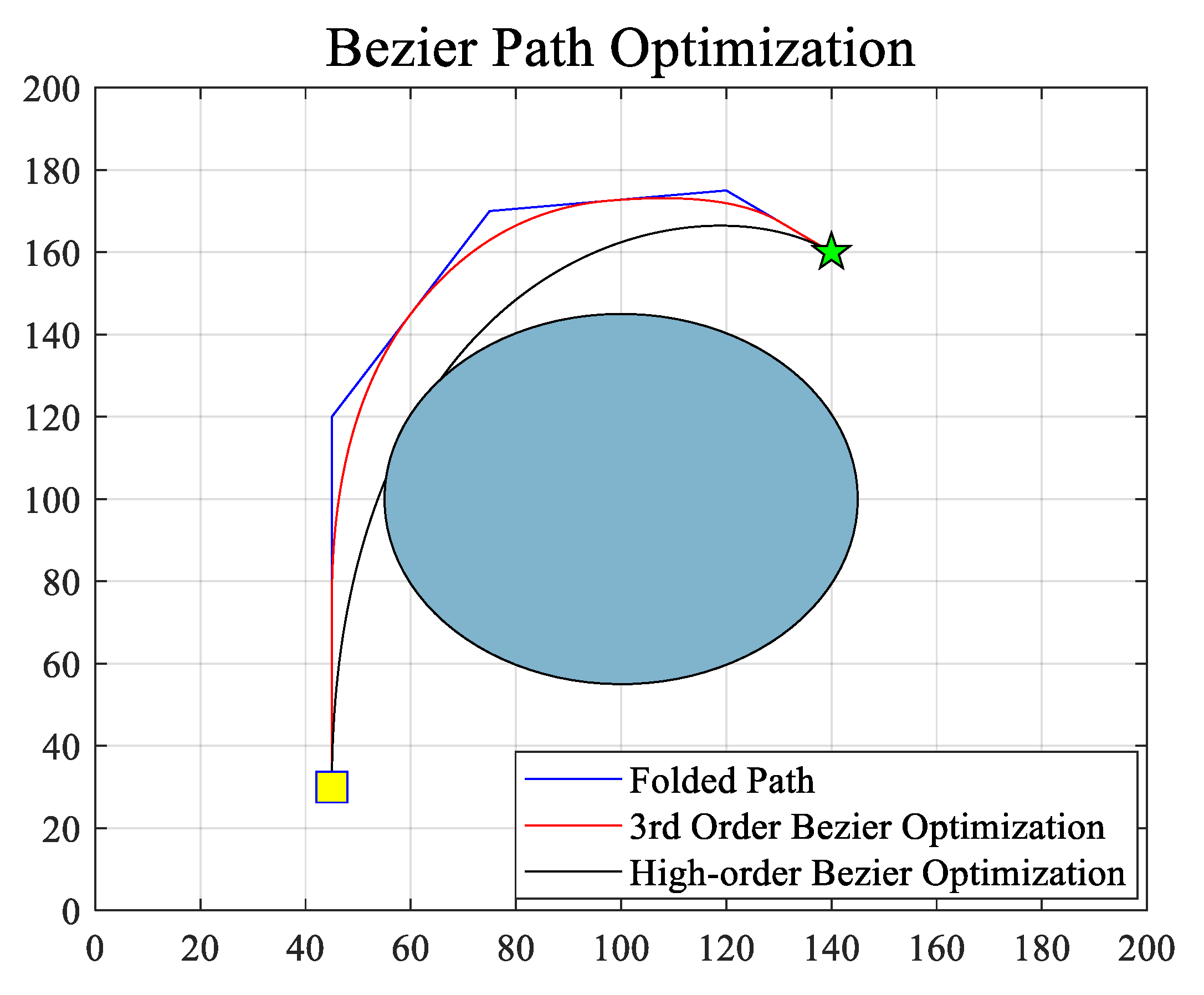
where B ( t ) denotes the Bézier curve connecting the key point P 0 ,   P 1 ,   , P n . The current common path optimization method uses high-order Bézier curves by extracting the floating points in the algorithm-generated folding path and then using its number as the basis for selecting the order of the Bézier curve to obtain a smooth continuous path. However, this method does not optimize the path in the case of curved path points because the optimized path will not be able to bypass the obstacles due to the characteristics of the higher-order Bézier curve. The optimized path does not work, so to deal with this problem, the obtained folding path is segmented, and the order of the Bézier curve is limited to 3. The optimization is performed only at the turning point of the folding path, and the straight-line part is retained in the original form so that the adaptation of the folding path generated by the algorithm can be maintained at the maximum and the purpose of smooth optimization can be achieved. The Bézier curve path optimization is shown in Figure 5.

2.4. SAHBES Iteration Steps

The final structure block diagram of the complete SAHBES and the specific iteration steps are shown in Figure 6.
Step 1: The parameters relating to the algorithms and map information are set: values are assigned to the population size N, the search range [lbx, ubx, lby, uby], the spatial dimension D, the maximum number of iterations T, and the coordinates O and the obstacle radius S of the obstacles.
Step 2: The location of each individual in the population is initialized and a random N × D dimensional matrix is generated as the initial population within the search range, storing the location information of the individuals.
Step 3: The population’s initial fitness value is calculated.
Each individual’s fitness value is calculated according to the fitness function F(P).
These are then sorted to select the smallest fitness in the population, denoted as Pbest, and its corresponding individual is denoted as PbestX.
Step 4: In the selection stage, individual positions are updated according to Equations (1) and (10), the self-adaptive control factor α’ is calculated using the decreasing function, and the population fitness is calculated after the update is completed. The individuals with better fitness than before are updated in their normal positions, and vice versa, and the replacement record operation is also performed for Pbest and PbestX.
Step 5: In the prey searching stage, the population position updated by Equation (1) is updated again according to Equation (2), and the population fitness is calculated after the update is completed. The individuals with better fitness than before are updated in their normal positions, and vice versa, and the replacement record operation is also performed for Pbest and PbestX.
Step 6: In the swooping stage, the population is sorted according to the fitness value according to Equation (11), and the individuals with poor fitness are updated once individually, and then the population position is updated as an entire group according to Equation (6), and the population fitness is calculated after the update is completed. The individuals with better fitness than before are updated in their normal positions, and vice versa, and the replacement record operation is also performed for Pbest and PbestX.
Step 7: The iterative process from step 4 to step 6 is repeated, the search is stopped when the termination condition is satisfied, and the global optimal solution PbestX is output.
Step 8: The generated paths’ key points (n) are extracted in floating points. Then, the generated fold paths are optimized by segmentation using third-order Bézier curves to derive the final paths.

3. Simulation Tests

In order to test the path planning performance of SAHBES more comprehensively, a variety of complex maps, including random distribution obstacles as well as trap obstacles, are set in this paper. In terms of the algorithm parameters, the total number of individuals in the population is set to 20, and the total number of iterations is 1000. The individual dimension can also be understood as the number of path points of the algorithm-generated paths, and the larger the value is, the smoother the paths generated by the algorithm will be. However, this will also increase the computing time significantly, so in order to improve the efficiency of the calculation, this individual dimension is set to 5 and combined with the curve optimization module to make the generated paths smoother. The fitness function also needs to be set to the value of ρ. Since the radius of obstacles varies in random charts, this paper sets ρ to 0.5 times the radius of obstacles.
In this paper, Self-Adaptive Particle Swarm Optimization (SAPSO), as well as conventional BES, are applied to global path planning as a control group to highlight the advantages of the proposed SAHBES in global path planning and optimized with Bézier curves, respectively, with the specific parameters shown in Table 2.
In the BES and SAHBES algorithms, α ,   R controls the shape of the spiral search trajectory of the individual algorithm in the search stage, and c 1 ,   c 2 reflects the late convergence strength of the algorithm in the swoop stage, which are taken as the default values in this paper: α = 10 ,   R = 1.5 ,   c 1 = c 2 = 2 .
c 1 ,   c 2 denotes the two learning factors, which take the default value of two. It acts similarly to α and is related to the upper limit of the number of iterations T, whose value varies with the number of iterations t. Vmax denotes the dynamic range of each variable in the particle swarm, which is set to 1 by default. The value of w is mathematically expressed as the following Equation (19):
w = w ( w 0.3 ) t / T

3.1. Path Planning Simulation with Obstacles

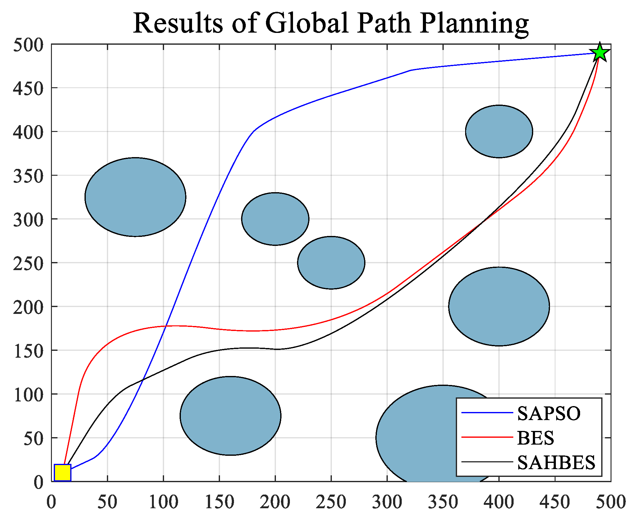
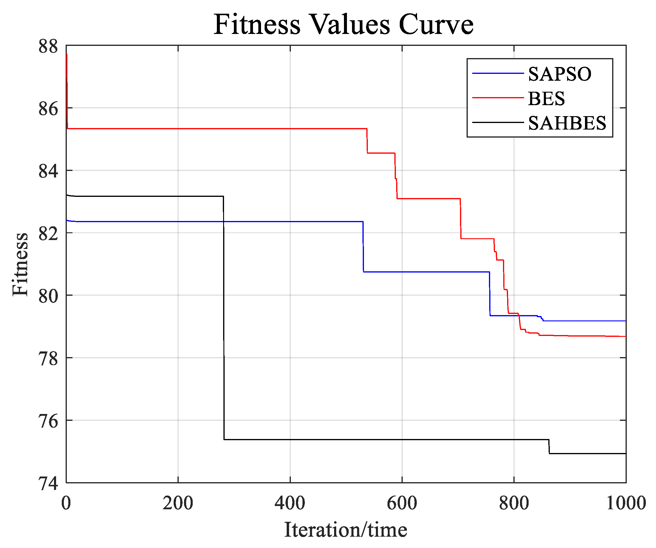
The distribution of the random obstacles chart is shown in Figure 7. Due to the obstacles’ dispersion, the population is easily affected by its low initial fitness during the initialization of the algorithm in the early search phase by falling into the local optimum. SAPSO and BES fall into the local optimum to varying degrees due to their low iteration efficiency. Although the generated paths meet the safety requirements, the curvature of the paths generated by BES is larger. At the same time, the SAHBES algorithm has a greater global search ability, and the fitness value is lower. Moreover, its fitness function and control factor are improved to generate smooth, safe, and better paths in the early iteration. The fitness values curves of the three algorithms are shown in Figure 8.

3.2. Trap Obstacle Path Planning Experiment

3.2.1. Trap Obstacles Simulation I

(1) Simulation Results
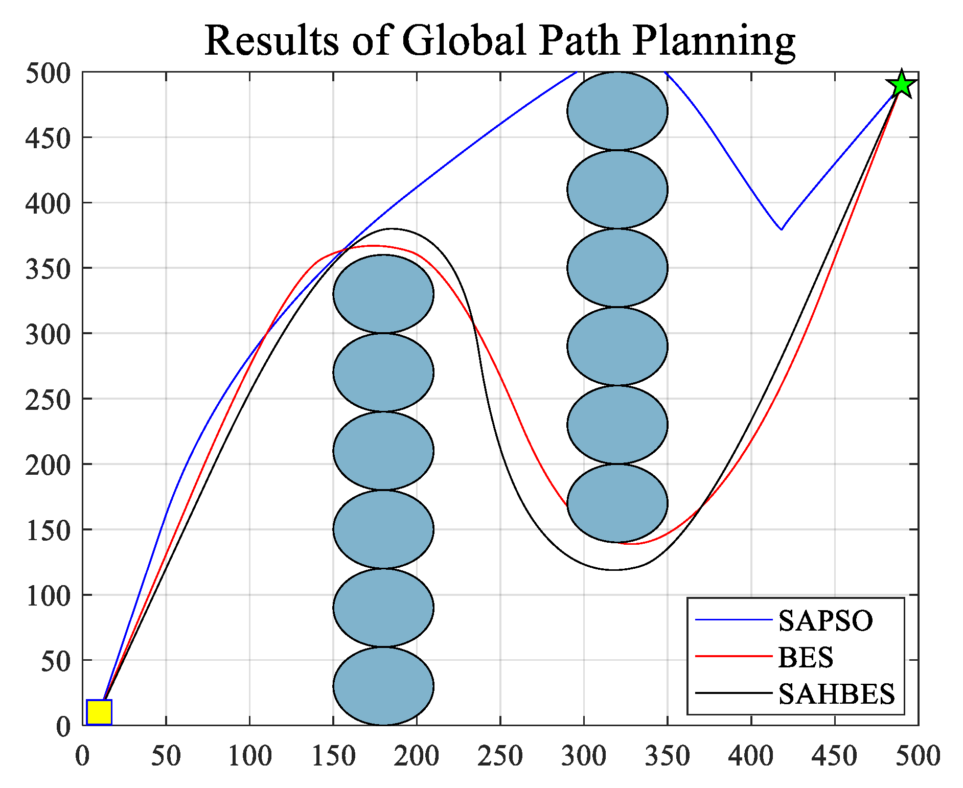
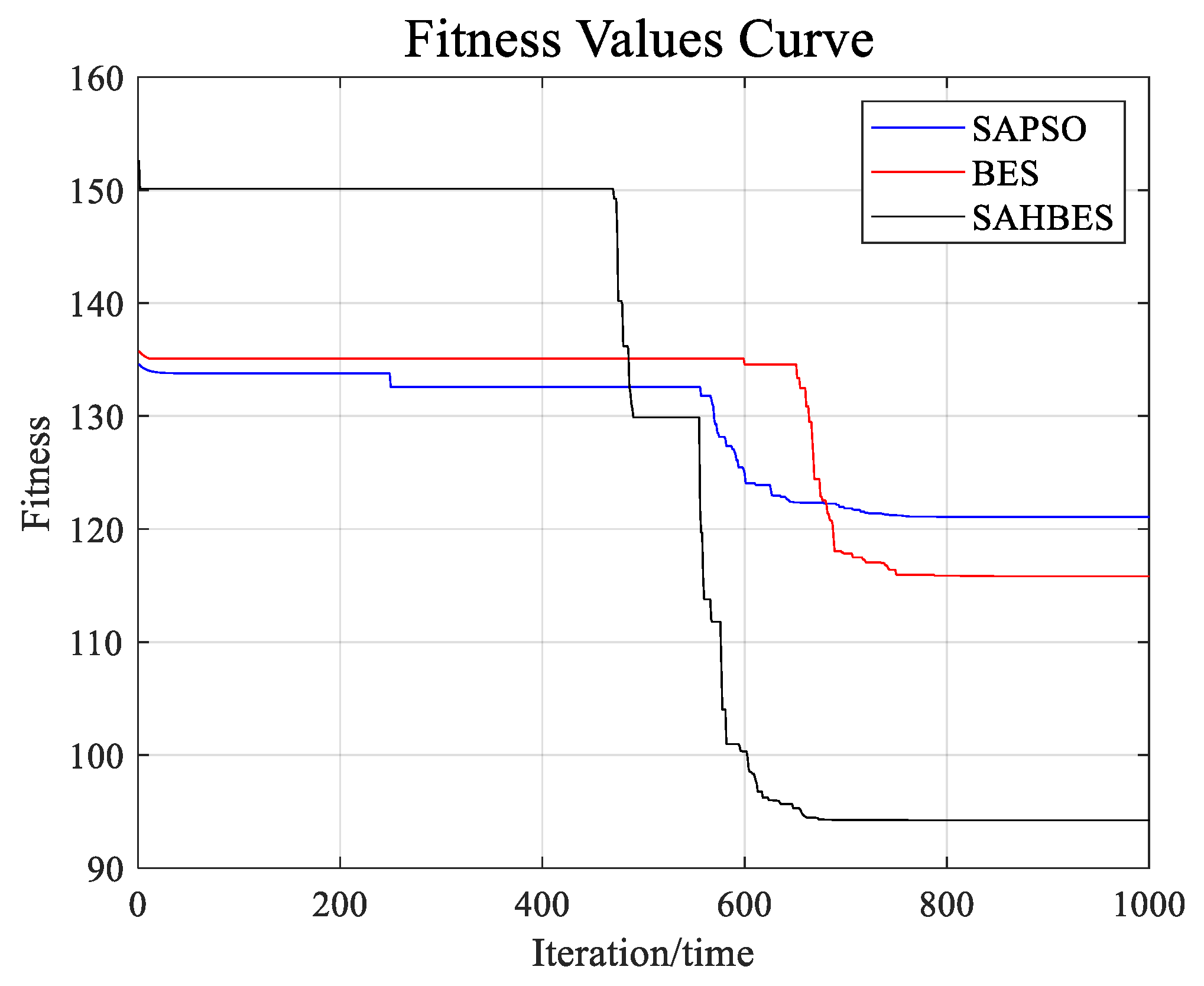
In order to compare the path planning effects of the three algorithms more obviously, three more complex trap obstacles charts are set up in this paper. The distribution of the Trap Obstacles Simulation I is shown in Figure 9. In this simulation, the search and generation of the optimal path are more difficult, and the global search ability and iteration efficiency of the algorithms are tested more. The values of the fitness functions of the three algorithms are shown in Figure 10.
(2) Conclusion of simulation results
From Figure 9, it can be seen that all three algorithms can find safe paths to avoid obstacles, but the path of SAPSO has an obvious turning point, which is caused by the two path points being too close to each other before the curve optimization. The path generated by SAHBES reduces the unnecessary and redundant parts of the path more than BES, which can be more economical in practical applications. However, by analyzing the fitness values, the global search ability of SAPSO and BES does not dominate when there are few optimal solutions. The optimal solution of BES is updated frequently but hardly reaches the optimum. SAHBES has more vital local search ability and greater convergence due to integrating part of the PIO into the swooping stage. However, it can be reflected only after decreasing in the later iterations.

3.2.2. Trap Obstacles Simulation II

(1) Simulation Results
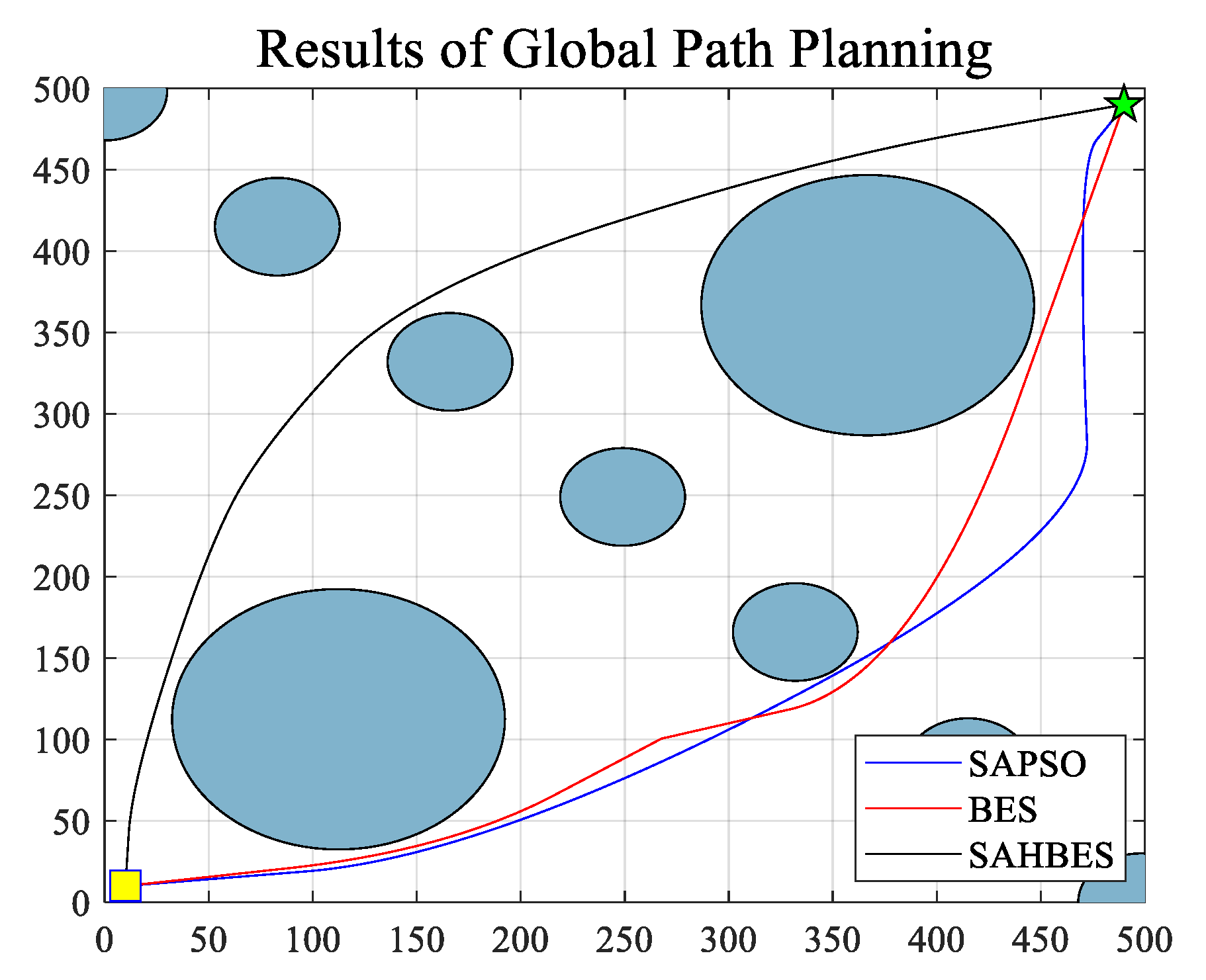
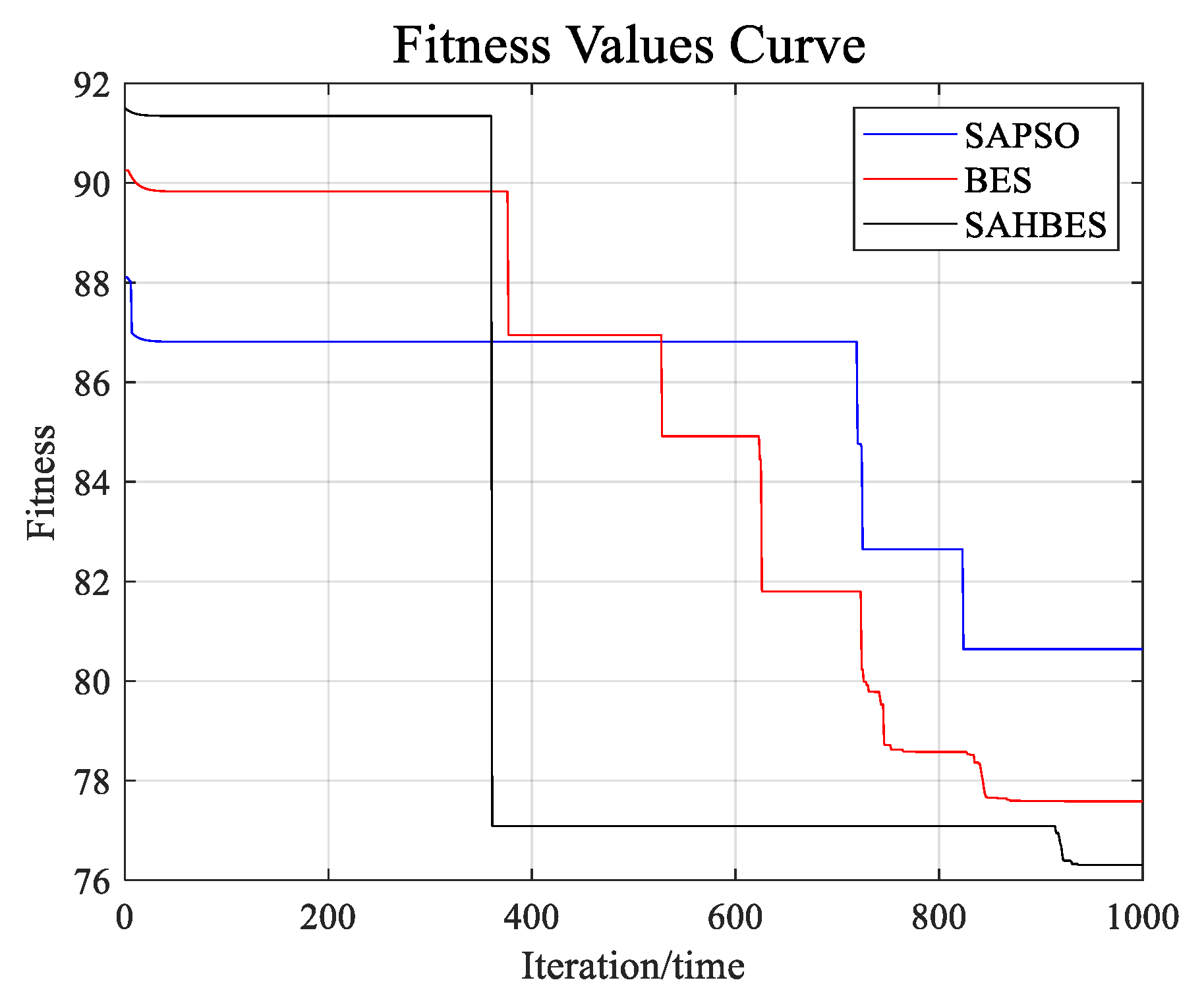
The Trap Obstacles Simulation II distribution is shown in Figure 11, and there is only one optimal path. The values of the fitness functions of the three algorithms are shown in Figure 12.
(2) Simulation Conclusions
Similarly to the Trap Obstacles Simulation I, Figure 11 shows that only one optimal path exists, but with a higher degree of folding complexity. SAHBES generates a path that can remain highly efficient and safe under the improved fitness function. While SAPSO does not find the optimal path and has the problem of falling into a local optimum, the path generated by BES fails to satisfy the safety condition and finds the optimal path after curve optimization and intersection with the obstacles. The advantage of SAHBES in global path planning can be observed.

3.2.3. Trap Obstacles Simulation III

(1) Simulation Results
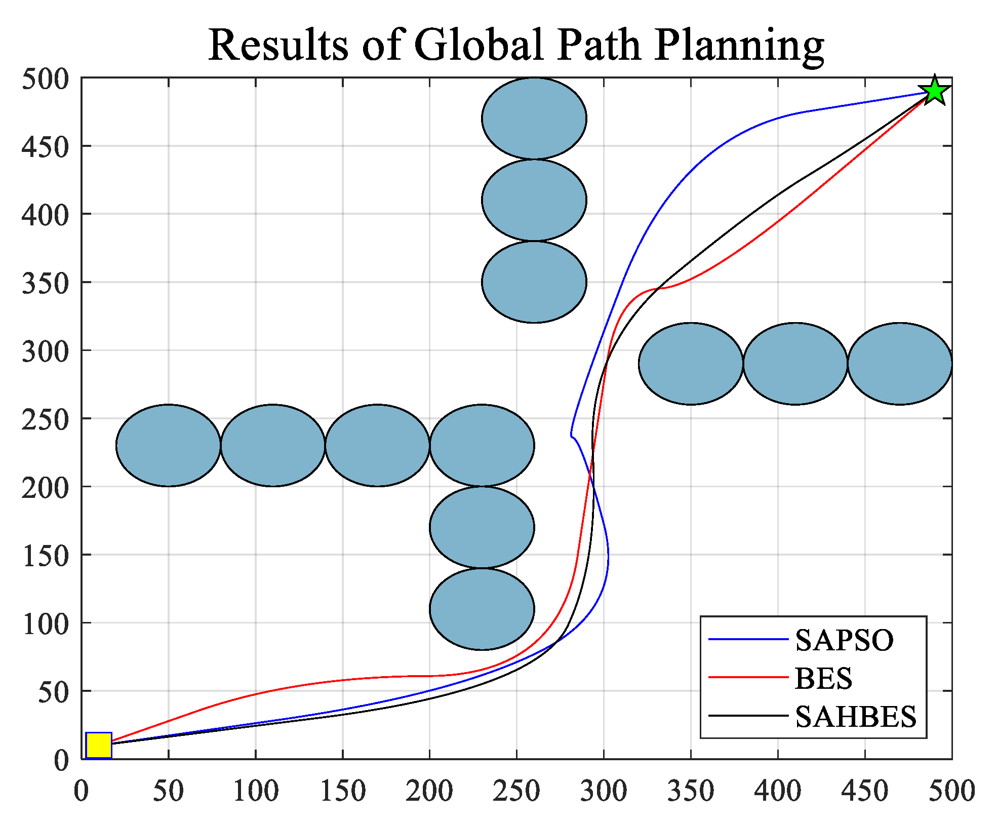
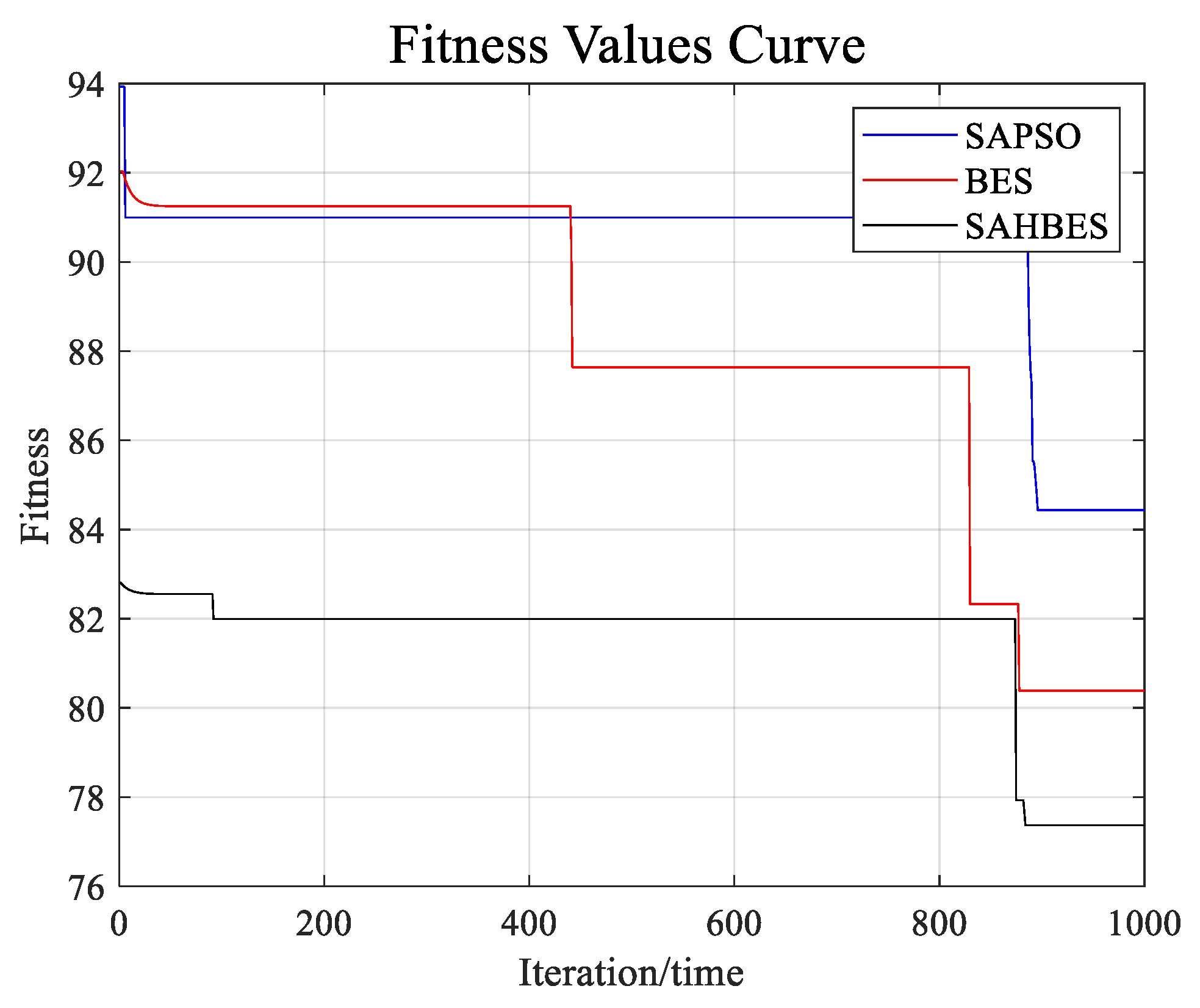
The distribution of the Trap Obstacles Simulation III is shown in Figure 13, and there are two optimal paths. The values of the fitness functions of the three algorithms are shown in Figure 14.
(2) Simulation Conclusions
Figure 13 shows the symmetric structure obstacles; there exist two optimal paths. The path generated by SAPSO has intersection points with the obstacles. The global optimization ability needs to be better and converge to the optimum. In contrast, BES generates paths that can maintain a safe distance from the obstacles, but the paths generated by this algorithm may have local optimum problems. SAHBES still performs the best, and, combined with the analysis of the fitness values curve (Figure 14), the algorithm has converged to an optimal solution similarly to BES in the middle of the iteration. At the end of the iteration, it can optimize further due to the effect of the self-adaptation factor.

4. Conclusions

This paper improves the algorithm structure of the basic BES. It proposes SAHBES by introducing self-adaptive control factors and incorporating a part of the ideas of PIO, which has good robustness, a higher convergence rate, and high iteration efficiency (77% higher than traditional BES) (The code of SAHBES can be found in Appendix A). In order to make the generated paths realistic, this paper also introduces a curve optimization module to optimize the generated fold paths using third-order Bézier curves. Compared with SAPSO and traditional BES, SAHBES also shows excellent performance in global path planning simulation tests and generates a continuous smooth path that meets the actual navigation situation. Moreover, the path is safe enough in terms of its distance and reliability, laying the foundation for unmanned ships’ path planning.
However, the multiple calculations of the fitness values in the algorithm structure lead to its high iteration efficiency but weak overall operation speed, which can be reconsidered to improve the algorithm structure further to decrease its operation time. In addition, this paper only verifies the superiority of SAHBES compared with traditional BES and its feasibility in global path planning. The simulation experiments are completed with the MATLAB platform, which can be considered for the application to real ships for further testing in future studies.

Author Contributions

Conceptualization, Y.C. and P.J.; methodology, W.W. and P.J.; software, C.W.; validation, Y.C., P.J. and W.W.; formal analysis, Y.C. and P.J.; investigation, Y.C.; resources, W.W.; data curation, Y.C., W.W. and C.W.; writing—original draft preparation, P.J.; writing—review and editing, W.W.; visualization, C.W.; supervision, Y.C.; project administration, C.W.; funding acquisition, C.W. All authors have read and agreed to the published version of the manuscript.

Funding

This work is supported by the National Natural Science Foundation of China (51909202), and the Funds for International Cooperation and Exchange of the National Natural Science Foundation of China (51920105014).

Institutional Review Board Statement

Not applicable.

Informed Consent Statement

Not applicable.

Data Availability Statement

Not applicable.

Conflicts of Interest

The authors declare no conflict of interest.

Appendix A

The code of SAHBES:
clc;
clear;
number_fun = ‘F’;
MaxIt = 100;
nPop = 50;
[low,high,dim,fobj] = Get_Functions(number_fun);
% st = cputime;
% Initialize Best Solution
BestSol.cost = inf;
for i = 1:nPop
         pop.pos(i,:) = low + (high-low).*rand(1,dim);
           pop.cost(i) = fobj(pop.pos(i,:));
        if pop.cost(i) < BestSol.cost
               BestSol.pos = pop.pos(i,:);
               BestSol.cost = pop.cost(i);
        end
end
  %disp(num2str([0 BestSol.cost]));
for t = 1:MaxIt
        %%                                  1- select_space
        [pop, BestSol, s1(t)] = select_space(t,MaxIt,fobj,pop,nPop,BestSol,low,high,dim);
        %%                                  2- search in space
        [pop, BestSol, s2(t)] = search_space(fobj,pop,BestSol,nPop,low,high);
        %%                                  3- swoop
    [pop, BestSol, s3(t)] = swoop(fobj,pop,BestSol,nPop,low,high,t,MaxIt);
                Convergence_curve(t) = BestSol.cost;
                %disp(num2str([t BestSol.cost]))
%          ed = cputime;
%          timep = ed-st;
end
%%
semilogy(Convergence_curve,‘-’);
xlabel(‘Iteration’)
ylabel(‘fitness’)
legend(’BES’)
%%
function [pop BestSol s1] = select_space(t,MaxIt,fobj,pop,npop,BestSol,low,high,dim)
Mean = mean(pop.pos);
% Empty Structure for Individuals
empty_individual.pos = [];
empty_individual.cost = [];
% lm= 2;
lm= 2-0.5*(t/MaxIt)^2;
s1 = 0;
for i = 1:npop
        newsol = empty_individual;
        newsol.pos= BestSol.pos+ lm*rand(1,dim).*(Mean - pop.pos(i,:));
        newsol.pos = max(newsol.pos, low);
        newsol.pos = min(newsol.pos, high);
        newsol.cost = fobj(newsol.pos);
        if newsol.cost < pop.cost(i)
              pop.pos(i,:) = newsol.pos;
              pop.cost(i)= newsol.cost;
              s1 = s1 + 1;
                  if pop.cost(i) < BestSol.cost
                    BestSol.pos= pop.pos(i,:);
                  BestSol.cost = pop.cost(i);
                  end
        end
end
end
function [pop, best, s1] = search_space(fobj,pop,best,npop,low,high)
Mean = mean(pop.pos);
a = 10;
R = 1.5;
% Empty Structure for Individuals
empty_individual.pos = [];
empty_individual.cost = [];
s1 = 0;
for i = 1:npop-1
        A = randperm(npop);
pop.pos = pop.pos(A,:);
pop.cost = pop.cost(A);
                [x, y] = polr(a,R,npop);
        newsol = empty_individual;
      Step = pop.pos(i,:) - pop.pos(i + 1,:);
      Step1 = pop.pos(i,:)-Mean;
      newsol.pos = pop.pos(i,:) +y(i)*Step + x(i)*Step1;
        newsol.pos = max(newsol.pos, low);
        newsol.pos = min(newsol.pos, high);
        newsol.cost = fobj(newsol.pos);
        if newsol.cost < pop.cost(i)
              pop.pos(i,:) = newsol.pos;
              pop.cost(i)= newsol.cost;
                            s1 = s1 + 1;
                        if pop.cost(i) < best.cost
                                best.pos= pop.pos(i,:);
                              best.cost = pop.cost(i);
                    end
        end
end
end
 
function [pop, best, s1] = swoop(fobj,pop,best,npop,low,high,t,MaxIt)
Mean = mean(pop.pos);
a = 10;
R = 1.5;
% Empty Structure for Individuals
empty_individual.pos = [];
empty_individual.cost = [];
s1 = 0;
%%
for i = 1:npop-1                                                 %sort the pigeons
                for j = i+1:npop
                        if pop.cost(:,i) > pop.cost(:,j)
                              temp_pos = pop.pos(i,:);
                              temp_cost = pop.cost(:,i);
                              pop.pos(i,:) = pop.pos(j,:);
                              pop.cost(:,i) = pop.cost(:,j);
                              pop.pos(j,:) = temp_pos;
                              pop.cost(:,j) = temp_cost;
                      end
              end
end
        npop1 = ceil(npop/2);                                  %remove half of the pigeons according to the landmark
        for m = (npop1 + 1):npop                                                                    %local searching
                        newsol.pos = pop.pos(m,:) + (2-0.5*(t/MaxIt)^2)*rand*(Mean-pop.pos(m,:));
        end
  for i = 1:npop
        newsol.cost = fobj(newsol.pos);
        if newsol.cost < pop.cost(i)
              pop.pos(i,:) = newsol.pos;
              pop.cost(i)= newsol.cost;
                        if pop.cost(i) < best.cost
                                  best.pos= pop.pos(i,:);
                                best.cost = pop.cost(i);
                        end
        end
  end
%%
for i = 1:npop
        A = randperm(npop);
pop.pos = pop.pos(A,:);
pop.cost = pop.cost(A);
                [x y] = swoo_p(a,R,npop);
        newsol = empty_individual;
      Step = pop.pos(i,:) - 2*Mean;
      Step1= pop.pos(i,:)-2*best.pos;
      newsol.pos = rand(1,length(Mean)).*best.pos + x(i)*Step + y(i)*Step1;
%        newsol.pos = (2*rand(1,length(Mean))-ones(1,length(Mean))).*best.pos + x(i)*Step + y(i)*Step1;
        newsol.pos = max(newsol.pos, low);
        newsol.pos = min(newsol.pos, high);
        newsol.cost = fobj(newsol.pos);
        if newsol.cost < pop.cost(i)
                pop.pos(i,:) = newsol.pos;
                pop.cost(i)= newsol.cost;
                            s1 = s1 + 1;
                        if pop.cost(i) < best.cost
                                best.pos= pop.pos(i,:);
                              best.cost = pop.cost(i);
                    end
        end
end
end
 
function [xR yR] = swoo_p(a,R,N)
th = a*pi*exp(rand(N,1));
r = th; %R*rand(N,1);
xR = r.*sinh(th);
yR = r.*cosh(th);
  xR = xR/max(abs(xR));
  yR = yR/max(abs(yR));
end
  function [xR yR] = polr(a,R,N)
%// Set parameters
th = a*pi*rand(N,1);
r = th + R*rand(N,1);
xR = r.*sin(th);
yR = r.*cos(th);
  xR = xR/max(abs(xR));
  yR = yR/max(abs(yR));
  end
function [lb,ub,dim,fobj] = Get_Functions(F)
switch F
        case ’F’%Branin Function
                fobj = @F17;
                lb = [−5,0];
                ub = [10,15];
                dim = 2;
 
end
end
  function o = F(x)
o = (x(2)-(x(1)^2)*5.1/(4*(pi^2)) + 5/pi*x(1)-6)^2 + 10*(1-1/(8*pi))*cos(x(1)) + 10;
  end

References

  1. Xie, S.; Chu, X.M.; Liu, C.G.; Wu, Q. A Review and Prospect of Ship Intelligent Collision Avoidance System. J. Trans. Inf. Saf. 2016. [Google Scholar] [CrossRef]
  2. Xie, X.L.; He, P.; He, A.; Xin, J.Y. Collision Avoidance Path Planning of Ships in Complicated Water Areas. J. Chongqing Jiaotong Univ. Nat. Sci. 2019, 38, 12. [Google Scholar]
  3. Iijima, Y.; Hagiwara, H. Results of collision avoidance maneuver experiments using a knowledge-based autonomous piloting system. J. Navig. 1991, 44, 194–204. [Google Scholar] [CrossRef]
  4. Tsou, M. Multi-target collision avoidance route planning under an ECDIS framework. Ocean Eng. 2016, 121, 268–278. [Google Scholar] [CrossRef]
  5. Zhang, G.; Deng, Y.; Zhang, W. Robust neural path-following control for under actuated ships with the DVS obstacles avoidance guidance. Ocean Eng. 2017, 143, 198–208. [Google Scholar] [CrossRef]
  6. Jeong, M.G.; Lee, E.B.; Lee, M.; Jung, J.Y. Multi-criteria route planning with risk contour map for smart navigation. Ocean Eng. 2019, 172, 72–85. [Google Scholar] [CrossRef]
  7. Huang, Y.M.; Chen, L.Y.; Van Gelder, P. Generalized velocity obstacle algorithm for preventing ship collisions at sea. Ocean Eng. 2019, 173, 142–156. [Google Scholar] [CrossRef]
  8. Yu, J.G.; Liu, Z.J.; Zhang, X.K. DCA-Based Collision Avoidance Path Planning for Marine Vehicles in Presence of the Multi-Ship Encounter Situation. J. Mar. Sci. Eng. 2022, 10, 529. [Google Scholar] [CrossRef]
  9. Chen, P.F.; Huang, Y.M.; Papadimitriou, E.; Mou, J.M.; Van Gender, P. Global path planning for autonomous ship: A hybrid approach of Fast Marching Square and velocity obstacles methods. Ocean Eng. 2020, 214, 107793. [Google Scholar] [CrossRef]
  10. Zhao, B.G.; Zhang, X.K.; Liang, C.L. A novel path-following control algorithm for surface vessels based on global course constraint and nonlinear feedback technology. Appl. Ocean Res. 2021, 111, 102635. [Google Scholar] [CrossRef]
  11. Guo, S.; Zhang, X.; Zheng, Y.; Du, Y. An Autonomous Path Planning Model for Unmanned Ships Based on Deep Reinforcement Learning. Sensors 2020, 20, 426. [Google Scholar] [CrossRef]
  12. Li, L.; Wu, D.; Huang, Y.; Yuan, Z.-M. A path planning strategy unified with a COLREGS collision avoidance function based on deep reinforcement learning and artificial potential field. Appl. Ocean Res. 2021, 113, 102759. [Google Scholar] [CrossRef]
  13. Ma, Y.; Hu, M.; Yan, X. Multi-objective path planning for unmanned surface vehicle with currents effects. ISA Trans. 2018, 75, 137–156. [Google Scholar] [CrossRef] [PubMed]
  14. Singh, Y.; Sharma, S.; Sutton, R.; Hatton, D.; Khan, A. A constrained A* approach towards optimal path planning for an unmanned surface vehicle in a maritime environment containing dynamic obstacles and ocean currents. Ocean Eng. 2018, 169, 187–201. [Google Scholar] [CrossRef] [Green Version]
  15. He, Z.; Liu, C.; Chu, X.; Negenborn, R.R.; Wu, Q. Dynamic anti-collision A-star algorithm for multi-ship encounter situations. Appl. Ocean Res. 2021, 118, 102995. [Google Scholar] [CrossRef]
  16. Xie, L.; Xue, S.; Zhang, J.; Zhang, M.; Tian, W.; Haugen, S. A path planning approach based on multi-direction A* algorithm for ships navigating within wind farm waters. Ocean Eng. 2019, 184, 311–322. [Google Scholar] [CrossRef]
  17. Tharwat, A.; Elhoseny, M.; Hassanien, A.E.; Gabel, T.; Kumar, A. Intelligent Bézier curve-based path planning model using Chaotic Particle Swarm Optimization algorithm. Clust. Comput. 2018, 22, 4745–4766. [Google Scholar] [CrossRef]
  18. Li, J.; Wang, H.; Zhao, W.; Xue, Y. Ship’s Trajectory Planning Based on Improved Multiobjective Algorithm for Collision Avoidance. J. Adv. Transp. 2019, 2019, 4068783. [Google Scholar] [CrossRef]
  19. Woo, J.; Kim, N. Collision avoidance for an unmanned surface vehicle using deep reinforcement learning. Ocean Eng. 2020, 199, 107001. [Google Scholar] [CrossRef]
  20. Xue, H. A quasi-reflection based SC-PSO for ship path planning with grounding avoidance. Ocean Eng. 2022, 247, 110772. [Google Scholar] [CrossRef]
  21. Han, S.; Wang, L.; Wang, Y.; He, H. A dynamically hybrid path planning for unmanned surface vehicles based on non-uniform Theta* and improved dynamic windows approach. Ocean Eng. 2022, 257, 111655. [Google Scholar] [CrossRef]
  22. Alsattar, H.A.; Zaidan, A.A.; Zaidan, B.B. Novel meta-heuristic bald eagle search optimisation algorithm. Artif. Intell. Rev. 2019, 53, 2237–2264. [Google Scholar] [CrossRef]
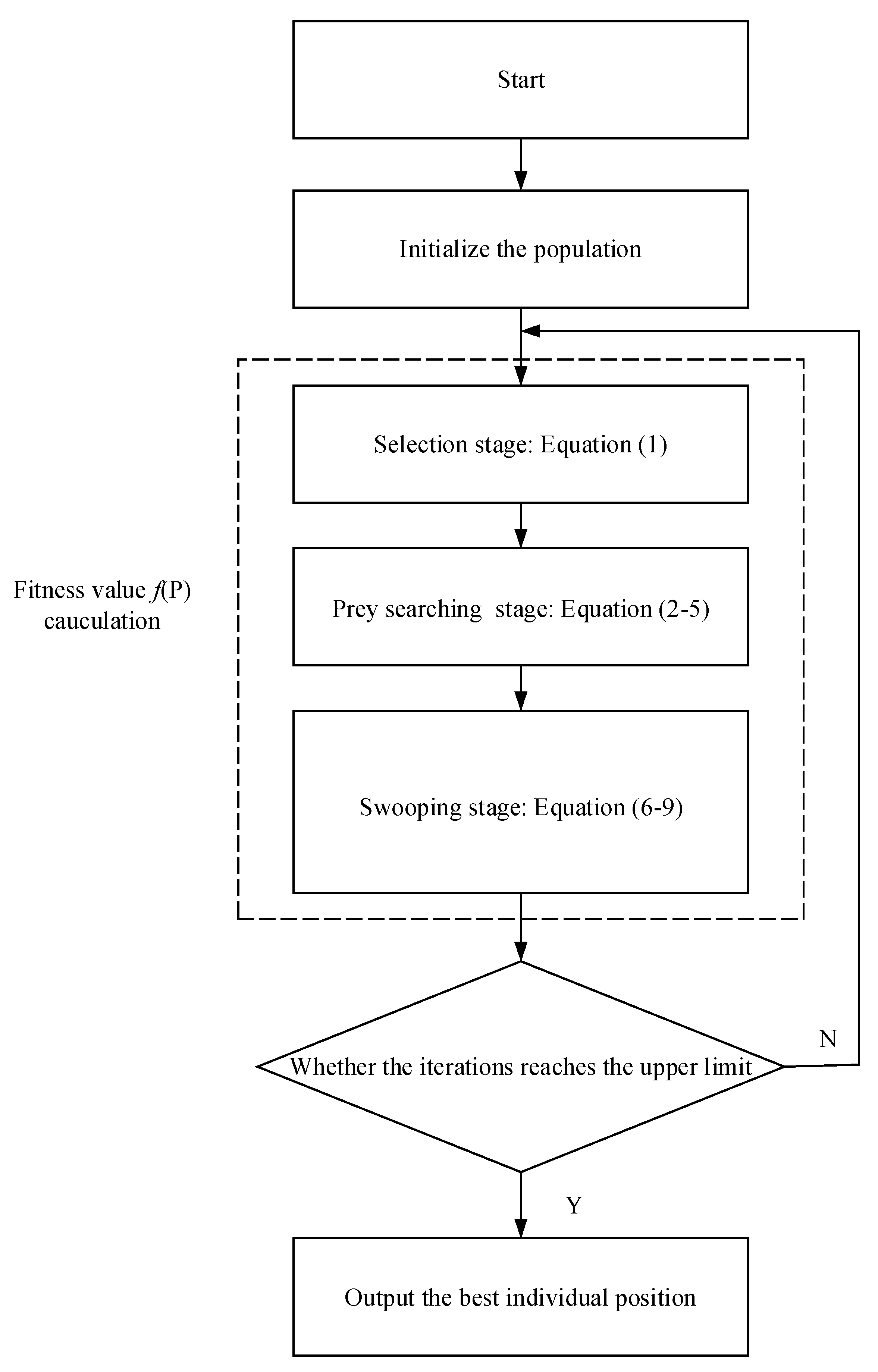
Figure 1. Process of traditional BES.
Jmse 11 00118 g001
Figure 2. Schematic diagram of test function.
Jmse 11 00118 g002
Figure 3. Comparison of the test functions’ fitness value curve.
Jmse 11 00118 g003
Figure 4. Principle diagram of fitness functions design.
Jmse 11 00118 g004
Figure 5. Bézier curve optimization schematic.
Jmse 11 00118 g005
Figure 6. Final SAHBES structure block diagram.
Jmse 11 00118 g006
Figure 7. Global path planning chart of random obstacles simulation.
Jmse 11 00118 g007
Figure 8. Comparison of the curves of the three algorithms’ fitness values.
Jmse 11 00118 g008
Figure 9. Global path planning chart of trap obstacles simulation I.
Jmse 11 00118 g009
Figure 10. Comparison of three algorithms’ fitness values of simulation I.
Jmse 11 00118 g010
Figure 11. Global path planning chart of trap obstacles simulation II.
Jmse 11 00118 g011
Figure 12. Comparison of the three algorithms’ fitness values of simulation II.
Jmse 11 00118 g012
Figure 13. Global path planning chart of trap obstacles simulation III.
Jmse 11 00118 g013
Figure 14. Comparison of the three algorithms’ fitness values of simulation III.
Jmse 11 00118 g014
Table 1. Function Maximum Optimization Test.
No.Function’s NameDimSearch IntervalMin-ValueMin-Coordinate
F1Ackley30[−10, 10]8.88178 × 10⁻¹⁶(2,2)
F2Penalized30[−5, 5]64([−5:1:5],1)
F3Schwefel 2.2630[−500, 500]−1675.93(421,421)
F4Rastrigin30[−5.12, 5.12]10,230([−5.02:1:2.98],[2.98:−1:−5.02])
Table 2. Algorithms’ parameters.
AlgorithmPopulation NumberMax IterationsFitness FunctionOther Parameters
SAPSO201000 f 1 ( P ) c1, c2, w, Vmax
BES201000 f 1 ( P ) c1, c2, α, R
SAHBES201000 F ( P ) c1, c2, α, R
Disclaimer/Publisher’s Note: The statements, opinions and data contained in all publications are solely those of the individual author(s) and contributor(s) and not of MDPI and/or the editor(s). MDPI and/or the editor(s) disclaim responsibility for any injury to people or property resulting from any ideas, methods, instructions or products referred to in the content.