
Simulation Study on the Sediment Dispersion during Deep-Sea Nodule Harvesting

 , , ,
, , ,
Abstract
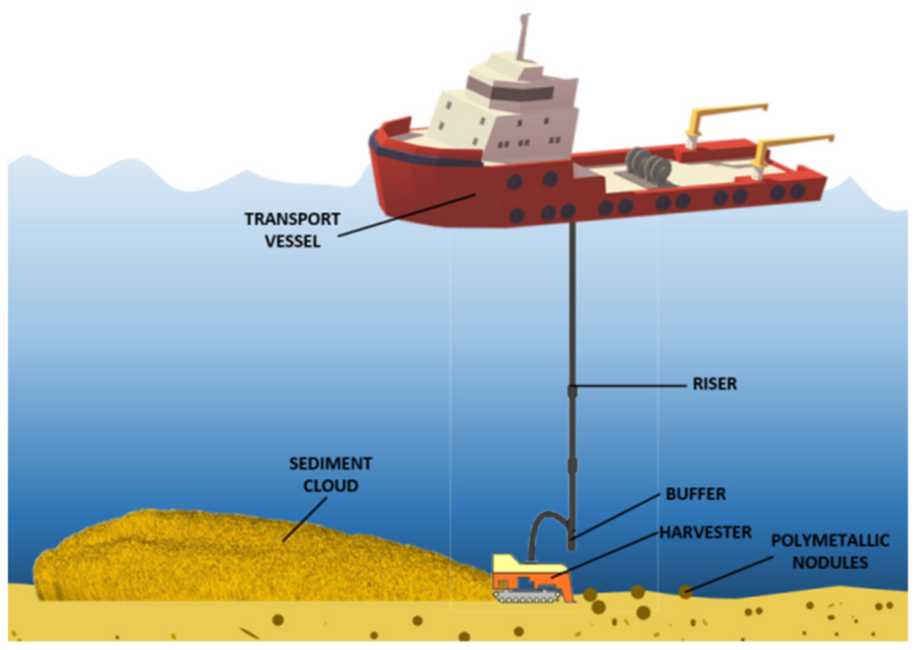
:1. Introduction
2. Methods
2.1. Numercial Simulation
2.1.1. Govern Equation
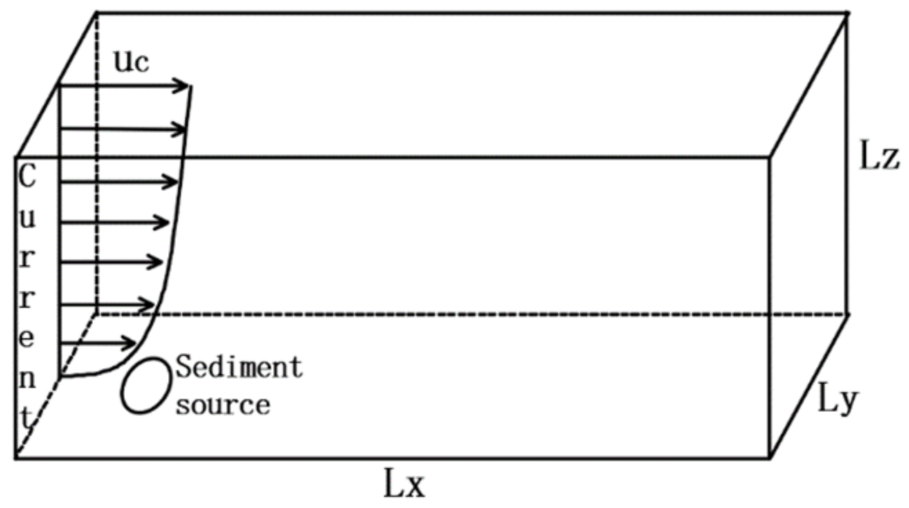
2.1.2. Simulation Model and Boundary Condition
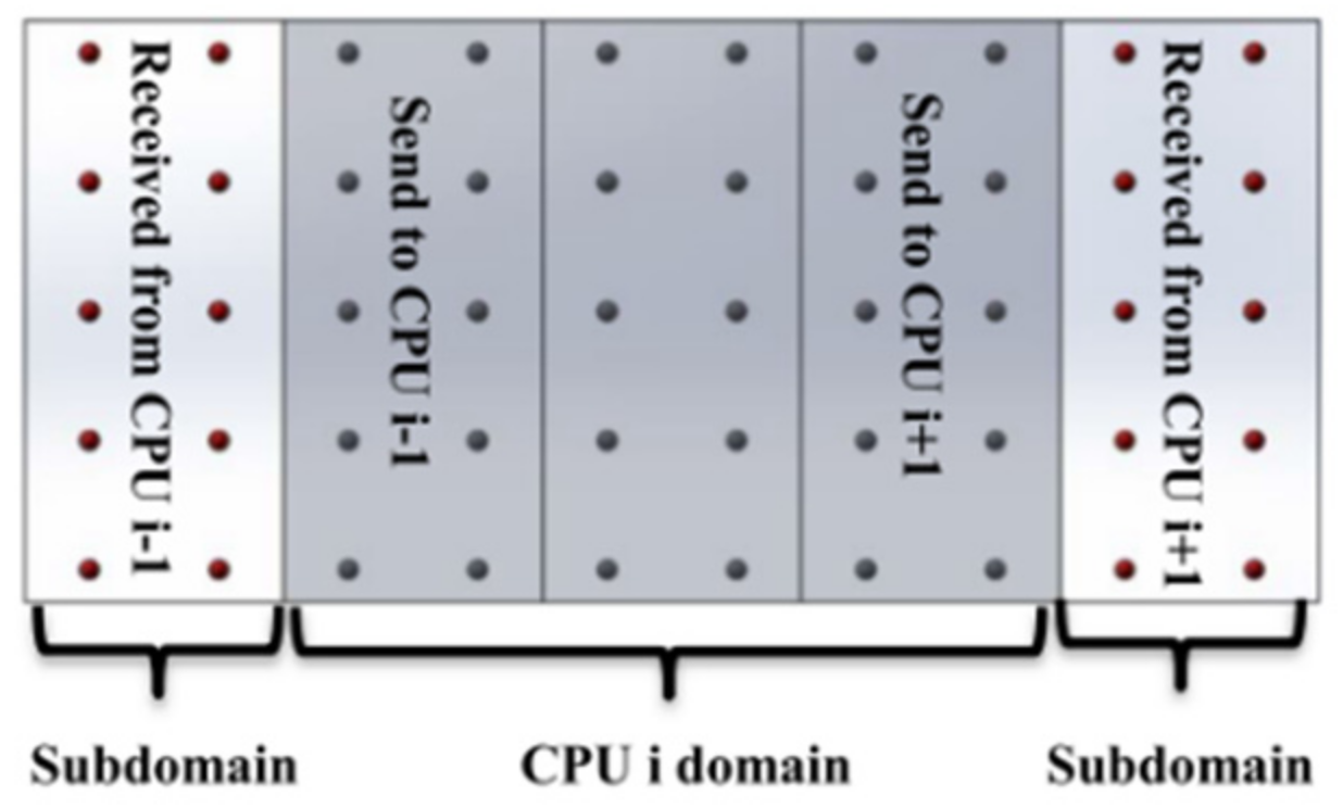
2.1.3. Smoothed Particle Hydrodynamics (SPH)
2.1.4. Simulation Parameters
2.2. Laboratory Experiments
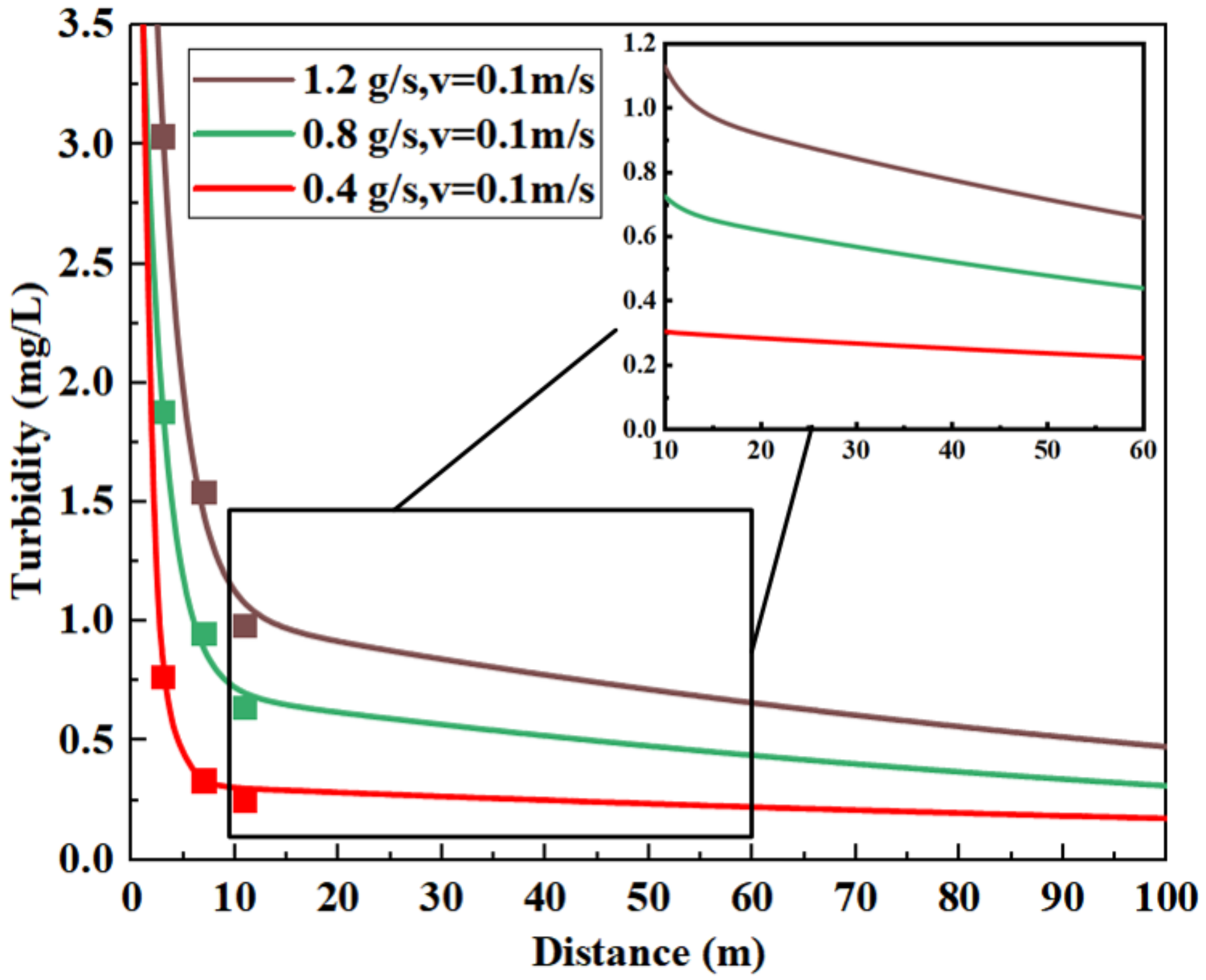
3. Results and Discussion
4. Conclusions
Author Contributions
Funding
Institutional Review Board Statement
Informed Consent Statement
Data Availability Statement
Conflicts of Interest
References
- Oebius, H.U.; Becker, H.J.; Rolinski, S.; Jankowski, J.A. Parametrization and evaluation of marine environmental impacts produced by deep-sea manganese nodule mining. Deep. Sea Res. Part II Top. Stud. Oceanogr. 2001, 48, 3453–3467. [Google Scholar] [CrossRef]
- Thiel, H.; Tiefsee-Umweltschutz, F. Evaluation of the environmental consequences of polymetallic nodule mining based on the results of the TUSCH Research Association. Deep. Sea Res. Part II Top. Stud. Oceanogr. 2001, 48, 3433–3452. [Google Scholar] [CrossRef]
- Smith, C.R.; Tunnicliffe, V.; Colaço, A.; Drazen, J.C.; Gollner, S.; Levin, L.A.; Mestre, N.C.; Metaxas, A.; Molodtsova, T.N.; Morato, T.; et al. Deep-Sea misconceptions cause underestimation of seabed-mining impacts. Trends Ecol. Evol. 2020, 35, 853–857. [Google Scholar] [CrossRef] [PubMed]
- Weaver, P.P.; Aguzzi, J.; Boschen-Rose, R.E.; Colaço, A.; de Stigter, H.; Gollner, S.; Haeckel, M.; Hauton, C.; Helmons, R.; Jones, D.O.; et al. Assessing plume impacts caused by polymetallic nodule mining vehicles. Mar. Policy 2022, 139, 105011. [Google Scholar] [CrossRef]
- Gillard, B.; Purkiani, K.; Chatzievangelou, D.; Vink, A.; Iversen, M.H.; Thomsen, L. Physical and hydrodynamic properties of deep sea mining-generated, abyssal sediment plumes in the Clarion Clipperton Fracture Zone (Eastern-Central Pacific). Elem. Sci. Anthr. 2019, 7, 5. [Google Scholar] [CrossRef] [Green Version]
- Aleynik, D.; Inall, M.E.; Dale, A.; Vink, A. Impact of remotely generated eddies on plume dispersion at abyssal mining sites in the Pacific. Sci. Rep. 2017, 7, 16959. [Google Scholar] [CrossRef] [Green Version]
- Rolinski, S.; Segschneider, J.; Sündermann, J. Long-term propagation of tailings from deep-sea mining under variable conditions by means of numerical simulations. Deep. Sea Res. Part II Top. Stud. Oceanogr. 2011, 48, 3469–3485. [Google Scholar] [CrossRef]
- Haalboom, S.; Schoening, T.; Urban, P.; Gazis, I.Z.; de Stigter, H.; Gillard, B.; Baeye, M.; Hollstein, M.; Purkiani, K.; Reichart, G.J.; et al. Monitoring of anthropogenic sediment plumes in the Clarion-Clipperton Zone, ne equatorial Pacific Ocean. Front. Mar. Sci. 2022, 9, 882155. [Google Scholar] [CrossRef]
- Baeye, M.; Purkiani, K.; de Stigter, H.; Gillard, B.; Fettweis, M.; Greinert, J. Tidally driven dispersion of a deep-sea sediment plume originating from seafloor disturbance in the DISCOL Area (SE-Pacific Ocean). Geosciences 2022, 12, 8. [Google Scholar] [CrossRef]
- Schoening, T.; Bodur, Y.; Köser, K. Automated image analysis to map the extent of deep-sea mining plumes reveals a larger impacted area compared to manual analysis. Sci. Rep. 2021. [Google Scholar] [CrossRef]
- Bian, X.; Litvinov, S.; Qian, R.; Ellero, M.; Adams, N.A. Multiscale modeling of particle in suspension with smoothed dissipative particle dynamics. Phys. Fluids 2012, 24, 012002. [Google Scholar] [CrossRef]
- Bian, X.; Litvinov, S.; Ellero, M.; Wagner, N.J. Hydrodynamic shear thickening of particulate suspension under confinement. J. Nonnewton. Fluid Mech. 2014, 213, 39–49. [Google Scholar] [CrossRef]
- Bertevas, E.; Tran-Duc, T.; Le-Cao, K.; Khoo, B.C.; Phan-Thien, N. A smoothed particle hydrodynamics (SPH) formulation of a two-phase mixture model and its application to turbulent sediment transport. Phys. Fluids 2019, 31, 103303. [Google Scholar] [CrossRef]
- Shi, H.; Yu, X.; Dalrymple, R.A. Development of a two-phase SPH model for sediment laden flows. Comput. Phys. Commun. 2017, 221, 259–272. [Google Scholar] [CrossRef]
- Gotoh, H.; Khayyer, A. On the state-of-the-art of particle methods for coastal and ocean engineering. Coast. Eng. J. 2018, 60, 79–103. [Google Scholar] [CrossRef] [Green Version]
- Yang, B.; Yang, F.; Liang, B.; Zhang, Q.; Wang, Z.; Wang, J. Numerical investigation of the interaction between the moving plate and sediment plume. Ocean. Eng. 2022, 248, 110839. [Google Scholar] [CrossRef]
- Tran-Duc, T.; Phan-Thien, N.; Khoo, B.C. A Three-dimensional smoothed particle hydrodynamics dispersion simulation of polydispersed sediment on the seafloor using a message passing interface algorithm. Phys. Fluids 2019, 31, 43301. [Google Scholar] [CrossRef]
- Stickel, J.J.; Powell, R.L. Fluid mechanics and rheology of dense suspensions. Annu. Rev. Fluid Mech. 2005, 37, 129–149. [Google Scholar] [CrossRef]
- Van der Werff, J.C.; De Kruif, C.G. Hard-sphere colloidal dispersions: The scaling of rheological properties with particle size, volume fraction, and shear rate. J. Rheol. 1989, 33, 421–454. [Google Scholar] [CrossRef]
- Sarkar, K.; Mazumder, B.S. Higher-order moments with turbulent length-scales and anisotropy associated with flow over dune shapes in tidal environment. Phys. Fluids 2018, 30, 106602. [Google Scholar] [CrossRef]
- Richardson, J.F.; Zaki, W.N. Sedimentation and fluidisation: Part I. Chem. Eng. Res. Des. 1997, 75, S82–S100. [Google Scholar] [CrossRef]
- Van Rijn, L.C. Principles of Sediment Transport in Rivers, Estuaries, and Coastal Seas; Aqua Publications: Amsterdam, The Netherlands, 1993. [Google Scholar]
- Tran-Duc, T.; Bertevas, E.; Phan-Thien, N.; Khoo, B.C. Simulation of anisotropic diffusion processes in fluids with smoothed particle hydrodynamics. Int. J. Numer. Methods Fluids 2016, 82, 730–747. [Google Scholar] [CrossRef]
- Grupe, B.; Becker, H.J.; Oebius, H.U. Geotechnical; sedimentological investigations of deep-sea sediments from a manganese nodule field of the Peru Basin. Deep Sea Res. Part II Top. Stud. Oceanogr. 2001, 48, 3593–3608. [Google Scholar] [CrossRef]
- Cabezón, R.M.; García-Senz, D.; Relaño, A. A one-parameter family of interpolating kernels for smoothed particle hydrodynamics studies. J. Comput. Phys. 2008, 227, 8523–8540. [Google Scholar] [CrossRef] [Green Version]
- Jankowski, J.A.; Malcherek, A.; Zielke, W. Numerical modeling of suspended sediment due to deep-sea mining. J. Geophys. Res. 1996, 101, 3545–3560. [Google Scholar] [CrossRef]
- Amon, D.J.; Rotjan, R.D.; Kennedy, B.R.; Alleng, G.; Anta, R.; Aram, E.; Edwards, T.; Creary-Ford, M.; Gjerde, K.M.; Gobin, J.; et al. My deep sea, my backyard: A pilot study to build capacity for global deep-ocean exploration and research. Philos. Trans. R. Soc. B 2022, 377, 20210121. [Google Scholar] [CrossRef]
- Caux, P.Y.; Moore, D.R.J.; MacDonald, D. Technical Appendix: Ambient Water Quality Guidelines (Criteria) for Turbidity, Suspended and Benthic Sediments; Government of British Columbia: Victoria, BC, Canada, 1997. [Google Scholar]
- Lin, Y.; Qin, H.; Guo, J.; Chen, J. Rheology of bentonite dispersions: Role of ionic strength and solid content. Appl. Clay Sci. 2021, 214, 106275. [Google Scholar] [CrossRef]
- Lin, Y.; Qin, H.; Guo, J.; Chen, J. Study on the Rheological Behavior of a Model Clay Sediment. J. Mar. Sci. Eng. 2021, 9, 81. [Google Scholar] [CrossRef]


| Parameters | Value | Unit |
|---|---|---|
| Ocean water density | 1045 | |
| Dry sediment density | 2650 | |
| Initial wetted sediment density | 1350 | |
| Critical stress for erosion | 0.18 | |
| Critical stress for deposition | 0.1 | |
| Bottom erosion rate | ||
| Vertical distribution | 2.0 | |
| Horizontal distribution | 10 | |
| Horizontal diffusivity | 0.01 | |
| Current velocity | 0.04 | |
| Lateral shift | 5 |
| Sizes | Settling Velocity (m/s) | Mass Fraction | |
|---|---|---|---|
| 1 | >100 | 5.367 | 0.14 |
| 2 | 60–100 | 2 | 0.10 |
| 3 | 20–60 | 8.15 | 0.36 |
| 4 | <20 | 2 | 0.40 |
| Parameters | ||||
|---|---|---|---|---|
| 0.4 g/s | 1.779 | −0.4451 | 0.29 | −0.004554 |
| 0.8 g/s | 4.606 | −0.4534 | 0.7353 | −0.008562 |
| 1.2 g/s | 6.449 | −0.3878 | 1.077 | −0.008167 |
Disclaimer/Publisher’s Note: The statements, opinions and data contained in all publications are solely those of the individual author(s) and contributor(s) and not of MDPI and/or the editor(s). MDPI and/or the editor(s) disclaim responsibility for any injury to people or property resulting from any ideas, methods, instructions or products referred to in the content. |
© 2022 by the authors. Licensee MDPI, Basel, Switzerland. This article is an open access article distributed under the terms and conditions of the Creative Commons Attribution (CC BY) license (https://creativecommons.org/licenses/by/4.0/).
Share and Cite
Lin, Y.; Weng, Z.; Guo, J.; Lin, X.; Phan-Thien, N.; Zhang, J. Simulation Study on the Sediment Dispersion during Deep-Sea Nodule Harvesting. J. Mar. Sci. Eng. 2023, 11, 10. https://doi.org/10.3390/jmse11010010
Lin Y, Weng Z, Guo J, Lin X, Phan-Thien N, Zhang J. Simulation Study on the Sediment Dispersion during Deep-Sea Nodule Harvesting. Journal of Marine Science and Engineering. 2023; 11(1):10. https://doi.org/10.3390/jmse11010010
Chicago/Turabian StyleLin, Yuan, Zixin Weng, Jin Guo, Xingshuang Lin, Nhan Phan-Thien, and Jian Zhang. 2023. "Simulation Study on the Sediment Dispersion during Deep-Sea Nodule Harvesting" Journal of Marine Science and Engineering 11, no. 1: 10. https://doi.org/10.3390/jmse11010010
APA StyleLin, Y., Weng, Z., Guo, J., Lin, X., Phan-Thien, N., & Zhang, J. (2023). Simulation Study on the Sediment Dispersion during Deep-Sea Nodule Harvesting. Journal of Marine Science and Engineering, 11(1), 10. https://doi.org/10.3390/jmse11010010