Solitary Wave Interaction with a Floating Pontoon Based on Boussinesq Model and CFD-Based Simulations

Abstract

A mathematical model of solitary wave interaction with a pontoon-type rigid floating structure over a flat bottom is formulated based on Boussinesq-type equations under weakly nonlinear dispersive waves. Based on the higher-order Boussinesq equations, the solitary wave equation is derived, and a semi-analytical solution is obtained using the perturbation technique. On the other hand, brief descriptions of the application of wave2Foam and OceanWave3D on the aforementioned problem are presented. The analytical solitary wave profiles in the outer region are compared with Computational Fluid Dynamics (CFD) and OceanWave 3D model simulations in different cases. The comparison shows a good level of agreement between analytical, wave2Foam, and OceanWave3D. In addition, based on the wave2Foam and coupled OceanWave3D model, the horizontal, vertical wave forces, and the pressure distributions around the pontoon are analysed. Further, the effect of the Ursell number, pontoon length, and water depth on the solitary wave profiles are analysed based on the analytical solution. The paper validates each of the three models and performs intercomparison among them to assess their fidelity and computational burden.

1. Introduction

In coastal and ocean engineering applications, nonlinear and shallow-water wave characteristics become important for coastal engineers in order to understand the influence of shallow water waves on nonlinear forms. One frequently used nonlinear water wave model is the solitary-wave model, in order to simplify some boundary value problems based on Boussinesq-type equations or nonlinear kind of equations associated without structures to analyse the characteristics and behaviour of solitary wave profiles by comparing various numerical wave models over flat or variable bottom topography (see [1,2,3,4]).

Due to the world’s energy requirement for future activities, the global community has driven towards design techniques for the study of wave energy devices for energy recovery from renewable sources like waves. Apart from the analysis of various environmental and design conditions, nonlinear wave load analysis on floating structures performed based on various analytical methods is of importance for achieving a better understanding of nonlinear waves with structures. Therefore, various Boussinesq models have been proposed for analysing the mutual interaction of nonlinear waves and floating structures in different water depths applications to marine activities and wave energy converters (see [5,6,7,8]).

Another interesting aspect of the nonlinear or solitary wave is the interaction with floating or submerged structures based on analytical, numerical, and experimental studies. Some of the relevant studies are discussed. An integrated analytical–numerical model was presented in [9] to simulate solitary wave interaction with a fixed and partially immersed body in two dimensions, and experiments were conducted to examine the effects of wave amplitude, structural submergence, and structural width on the transmitted and reflected waves. The interactions between solitary waves and structures of single and twin rectangular cylinders were studied to analyse the hydrodynamic forces with different incoming wave amplitudes based on a finite element method (FEM) in two dimensions (see [10]). The FEM-based code has also been used in coastal engineering studies to investigate the solitary wave impact on other types of structures (see [11,12]). The shoaling of broad-crested internal solitary waves using immersed boundary method was studied in [13], and they concluded that different solitary wave breaking mechanisms are related to the internal Iribarren number.

On the other hand, several researchers have simulated the floating structures based on a numerical CFD model in the interaction of solitary waves using OpenFOAM solver. For instance, the impact of solitary waves on a simplified bridge deck model without girder in [14], whereas another bridge model with girders, both experimentally and with CFD simulations, was studied in [15]. Another influential experimental investigation using a 1:10th scale model of periodic wave impact on a bridge was conducted in [16]. Additionally, the analysis of the impact of the solitary wave on straight bridge decks was performed in larger-scale (1:5) experiments in [17,18]. A modification of the solitary wave generation method proposed by [19] was proposed by [20]. Lather, in ref. [21], confirmed that the method proposed by [19] works better than Goring’s method (see [20]). However, their soliton generated in the experimental facility was off from the target by 10%. The solitary wave interaction with a vegetated platform breakwater in the framework of the 2D numerical model using a macroscopic approach based on OlaFlow solver was studied in [22]. The dispersive characteristics of solitary waves while propagating over a sloping area were studied in [23]. Although numerous previous studies have been performed for solitary waves, each of the studies had a different target, and the analysis of the results was performed based on the target. The study of the solitary wave interaction with a breakwater and the subsequent results remain to be investigated in detail.

In addition to analytical studies, a floating fixed box based on a CFD model was simulated and compared the results against analytical and experimental model results in different cases (see [24]). A Boussinesq model associated with wave diffraction by a floating cylinder and results were compared with CFD model simulations in [7,8]. On the other hand, very recently, a comparison of solitary waves over flat- and variable-bottom topographies was performed between Boussinesq model and CFD simulations in [4]. However, studies focusing on the interaction of solitary waves with a floating pontoon-type structure based on Boussinesq formulation are very few. The study of solitary wave interaction considering the viscous effect and their effect on load predictions are also not common.

Therefore, in the present paper, solitary wave interaction with a pontoon-type floating structure over the flat bottom is presented based on semi-analytical, CFD and coupled (OceanWave 3D) model simulations. The paper is organized as follows: Section 2 presents the mathematical model formulation based on Boussinesq equations, and a solitary wave solution in the outer region is obtained. Section 3 discusses the coupled model set up between CFD and OceanWave 3D, and their importance. Section 4 presents a comparison of the free-surface solitary wave profiles among analytical, CFD, and OceanWave 3D model simulations. Section 5 analyses the wave forces, pressure distributions around the floating pontoon, wave energy analysis and further, the effect of Ursell number, pontoon length, and water depth on the solitary wave profiles are presented from the analytical solution. Finally, some significant conclusions are discussed in Section 6.

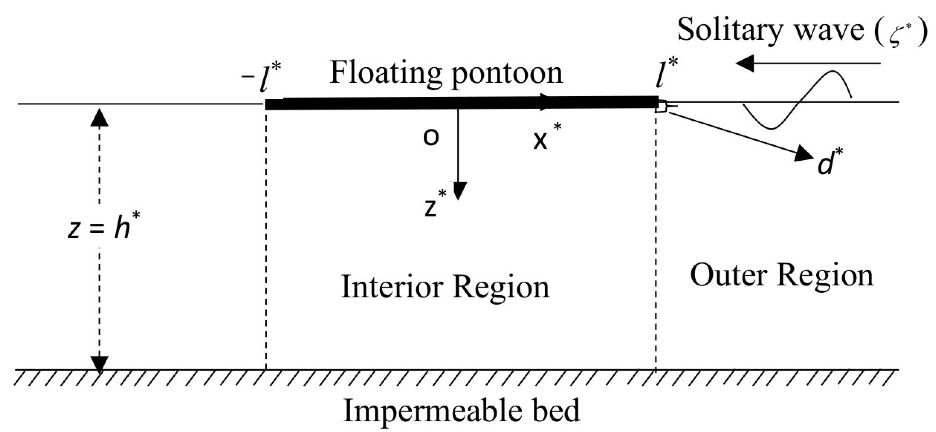
2. Mathematical Model Based on Boussinesq Equations

The mathematical model of the aforemention model is in a three-dimensional Cartesian coordinate system (x*, y*, z*), with x*-y* being the horizontal plane and z* pointing downward. The fluid occupies the region −h* < z* < 0, −∞ < x*< ∞ and a pontoon of length 2l* is floating at z* = 0 with draft d* and is balanced by the neutral buoyance over water depth at z = −h*, where ‘*’ indicates a dimensional variable. Hence, the fluid region is divided into two regions: an interior region that corresponds to the area below the pontoon and an outer region (incident wave region) (see Figure 1). The velocity potential and the free surface elevation in the outer region are denoted by Φ* and ${\zeta }^{*}$, respectively. Further, the fluid is assumed to be inviscid, incompressible, and the motion is irrotational and simple harmonic in time with angular frequency ω. In the case of long waves, two important non-dimensional parameters characterize the problem: the nonlinearity parameter $\epsilon =a_0/h_0$ and the dispersion parameter $\mu =h_0/\lambda$, where $h$ is the length representative of the depth scaled by $h_0$, $\lambda$ is the typical wavelength, and $a_0$ is the representative wave amplitude. The expressions for the non-dimensional quantities associated with the above variables are deferred here as it is quite common sense in the ocean engineering field.

In this mathematical model, the right-hand referencing frame has its x-axis pointing in the positive (right) direction, the z-axis is pointing downward negative direction, and the y-axis is expanding laterally. The coordinate origin is located at the water level of the undisturbed fluid region. The non-dimensionalised boundary-value problem can be formulated as the governing equation and associated boundary conditions. These equations are listed as follows:

$${\mu }^2{\nabla }^2\mathsf{\Phi }+{\mathsf{\Phi }}_{zz}=0\mathrm{for}-h\le z\le \epsilon \zeta ,$$

(1)

where ${\nabla }^2$ is the two-dimensional Laplacian operator in the horizontal plane.

The non-dimensional kinematic conditions in the outer region (free surface) region is given by

$${\mathsf{\Phi }}_z={\mu }^2({\zeta }_t+\epsilon \nabla \mathsf{\Phi }\nabla \zeta )\mathrm{at}z=\epsilon \zeta .$$

(2)

The non-dimensional dynamic condition is read as:

$${\mathsf{\Phi }}_t+g\zeta +\frac{1}{2}\epsilon {\left|\nabla \mathsf{\Phi }\right|}^2+\frac{U_r}{2}{\mathsf{\Phi }}_z^2=0\mathrm{at}z=\epsilon \zeta ,x\in (l,\infty ),$$

(3)

where $U_r=\epsilon /{\mu }^2$ is known as the Ursell number (as in [7]). The boundary condition on the pontoon cover yields

$${\mathsf{\Phi }}_z=0\mathrm{at}x\in (-l,l),z=d,$$

(4)

where the subscripts ‘z’ and ‘$t$’ are denote to the partial derivatives with respect to z and $t$, respectively.

Next, the bottom boundary condition at $z=-h$ is given by

$${\mathsf{\Phi }}_z=0\mathrm{at}z=-h.$$

(5)

Now, integrating Equation (1) w. r. t. z and using boundary conditions (2) and (4), the following is obtained:

$${\zeta }_t=-\nabla .\left[{\displaystyle \underset{-h}{\overset{\epsilon \zeta }{\int }}\nabla .\mathsf{\Phi }dz}\right]\mathrm{for}x\in (l,\infty ).$$

(6)

The next subsections will present the governing equation and boundary conditions in the interior region and solitary wave solutions in the outer region.

2.1. Governing Equations of the Interior Region and Matching Conditions

For the interior region beneath the pontoon, as shown in Figure 1, the velocity potential ${\mathsf{\Phi }}^I(x,z;t)$ satisfies the Laplace equation

$$\left(\frac{{\partial }^2}{\partial x^2}+\frac{{\partial }^2}{\partial z^2}\right){\mathsf{\Phi }}^I=0\mathrm{on}-h\le z\le -d.$$

(7)

The kinematic boundary conditions underneath the pontoon can be applied as follows:

$$\frac{\partial {\mathsf{\Phi }}^I}{\partial z}=0\mathrm{at}z=-d.$$

(8)

The matching conditions applied to the velocities and velocity potentials at the interface $x=l$ between the outer and interior fluid domains, as:

$$\frac{\partial {\mathsf{\Phi }}^O}{\partial x}=0\mathrm{for}-d\le z\le \epsilon \zeta .$$

(9)

where Equation (9) holds because the wave cannot overtop the pontoon.

$${\mathsf{\Phi }}^O={\mathsf{\Phi }}^I\mathrm{for}-h\le z\le -d,$$

(10)

$$\frac{\partial {\mathsf{\Phi }}^O}{\partial x}=\frac{\partial {\mathsf{\Phi }}^I}{\partial x}\mathrm{for}-h\le z\le -d.$$

(11)

The next subsection derives the solitary waveform in the outer region based on second-order approximation and using a depth-integrated approach.

2.2. Velocity Potential in Interior Region

Based on the method of separation of variables, the analytical solution of the velocity potentials in the interior region is expressed by solving the Laplace Equation (7) along with the boundary conditions (4) and (8) can be expressed as:

$${\mathsf{\Phi }}^I(x,z;t)={\displaystyle \sum _{n=0}^{\infty }\{A_n\cosh ({\beta }_{n}x)+B_n\sinh ({\beta }_{n}x)\}\cos {\beta }_n(z+h)},$$

(12)

where ${\beta }_n=n\pi /(h-d)$ and $\cos {\beta }_n(z+h)$ are the eigenfunctions and are orthogonal over the interval $-h\le z\le -d$.

2.3. Solitary Waveform $\zeta$ in Outer Region

The velocity potential $\mathsf{\Phi }(x,y,z;t)$ is expanded in powers of ${\mu }^2$ as follows:

$$\mathsf{\Phi }(x,y,z;t)={\displaystyle \sum _{n=0}^{\infty }{\mu }^{2n}\frac{{(z+h)}^{2n}}{(2n)!}{\nabla }_n^2{\phi }_n(x,y;t)}\mathrm{for}x\in (l,\infty ),$$

(13)

where $\mathsf{\Phi }(x,y,z;t)$ satisfies Equations (1) and (5). The higher-order Boussinesq equations are obtained by substituting Equation (13) into Equations (2) and (3) and on simplification and taking into account terms up to the order ${\epsilon }^2,\epsilon {\mu }^2,{\mu }^4$, as follows:

$$\begin{array}{ll}{\nabla }^2\phi -{\phi }_{tt}=& \frac{\epsilon }{2}{(\nabla \phi )}_t^2+\epsilon (\nabla \phi )(\nabla {\phi }_t)+\epsilon {\phi }_t{\nabla }^2\phi +\frac{{\mu }^2}{6}{\nabla }^4\phi -\frac{{\mu }^2}{2}{\nabla }^2{\phi }_{tt}+\frac{{\epsilon }^2}{2}(\nabla \phi )(\nabla {(\nabla \phi )}^2)\\ & +\frac{{\epsilon }^2}{2}{\nabla }^2\phi (\nabla \phi )+\frac{\epsilon {\mu }^2}{2}{\left\{{(\nabla \phi )}^2-{\phi }_t{\nabla }^2{\phi }_t-(\nabla \phi )(\nabla {\nabla }^2\phi )\right\}}_t-\frac{\epsilon {\mu }^2}{2}(\nabla {\nabla }^2\phi )(\nabla {\phi }_t)\\ & -\frac{\epsilon {\mu }^2}{2}(\nabla {\nabla }^2{\phi }_t)(\nabla \phi )-\frac{\epsilon {\mu }^2}{2}({\nabla }^2\phi )({\nabla }^2{\phi }_t)+\frac{\epsilon {\mu }^2}{2}{\phi }_t{\nabla }^4\phi +o({\epsilon }^2,\epsilon {\mu }^2,{\mu }^4),\mathrm{for}x\in (l,\infty ),\end{array}$$

(14)

$$\begin{array}{ll}\zeta =& {\phi }_t+\frac{{\mu }^2}{2}{\nabla }^2{\phi }_t+{\nabla }^2.{\phi }_t+\frac{\epsilon }{2}{(\nabla .\phi )}^2-\frac{\epsilon {\mu }^2}{2}\left\{{(\nabla .\phi )}^2-(\nabla .\phi )(\nabla {\nabla }^2.\phi )-{\phi }_t{\nabla }^2{\phi }_t\right\}\\ & +o({\epsilon }^2,\epsilon {\mu }^2,{\mu }^4),\mathrm{for}x\in (l,\infty )\end{array}$$

(15)

Now, the solitary waveform ($\zeta$) and velocity potential $\phi$ are the solutions of the above Equations to the lateral boundary at $x=l$ ($l<x<\infty$ and left going) can be expressed as:

$$\zeta (x;t)=\frac{3}{4}\left\{\left(\frac{4}{3}-\epsilon \right){\mathrm{sech}}^2\alpha (x-ct-l)+\epsilon {\mathrm{sech}}^4\alpha (x-ct-l)\right\},$$

(16)

$$\phi (x;t)=\frac{\tanh \alpha (x-ct-l)}{\alpha c}+\epsilon \tanh \alpha (x-ct-l)\left[\frac{1}{3}{\tanh }^2\alpha (x-ct-l)-\frac{1}{4}\right],$$

(17)

where $c=(1/2)(2+\epsilon )$ is the wave celerity and $\alpha =(\sqrt{3}/16)(8-5\epsilon )\sqrt{U_r}$.

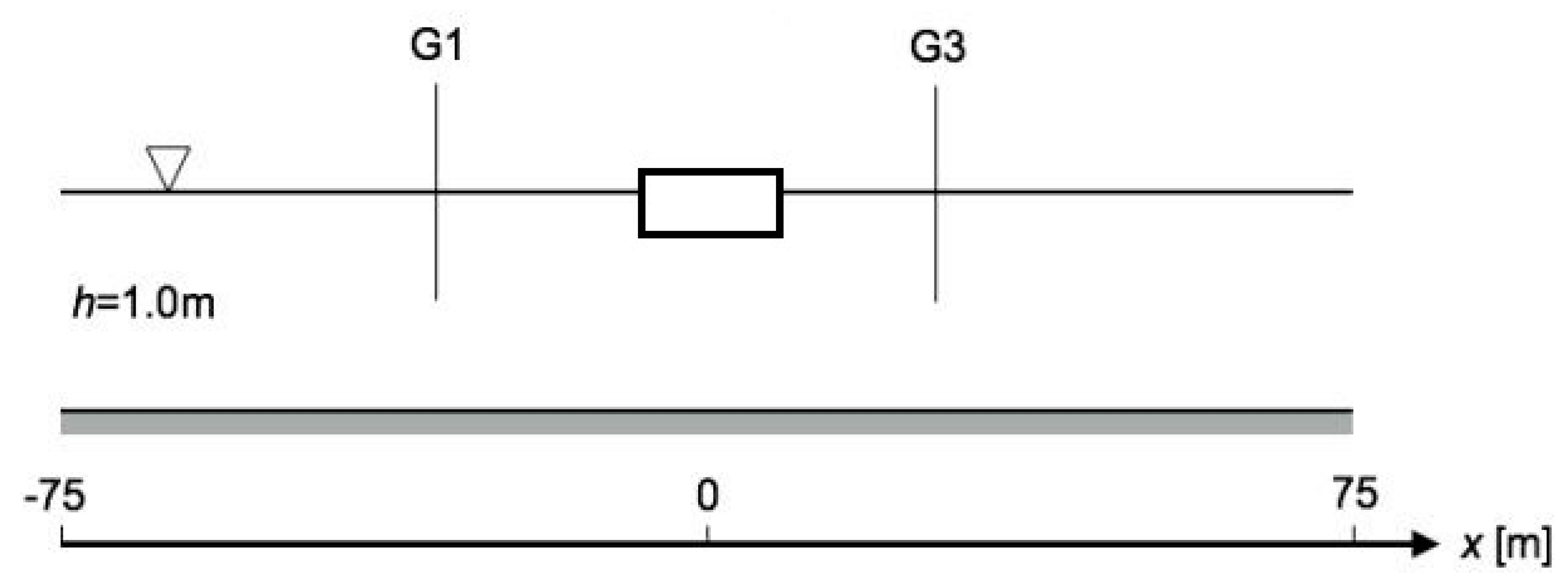
3. Description of Numerical Models

In this section, the brief descriptions of the numerical models based on CFD and OceanWave3D along with their model set up for the solitary wave interaction with a fixed floating pontoon are presented in the subsequent sections.

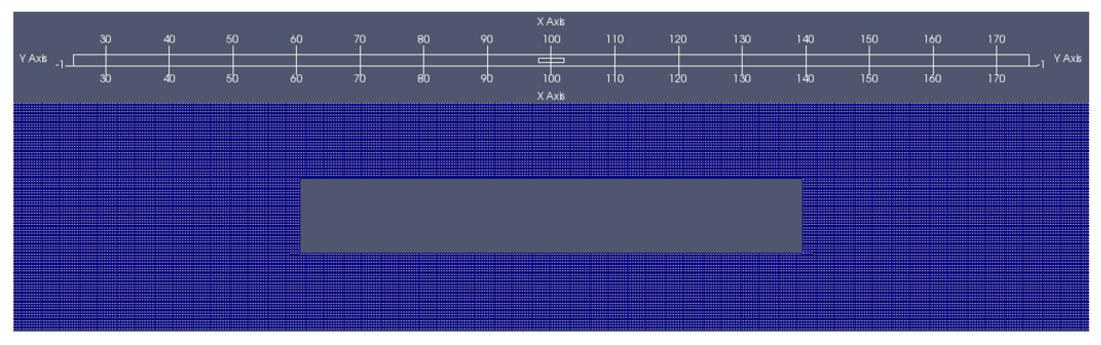
3.1. Brief Description of the CFD Model

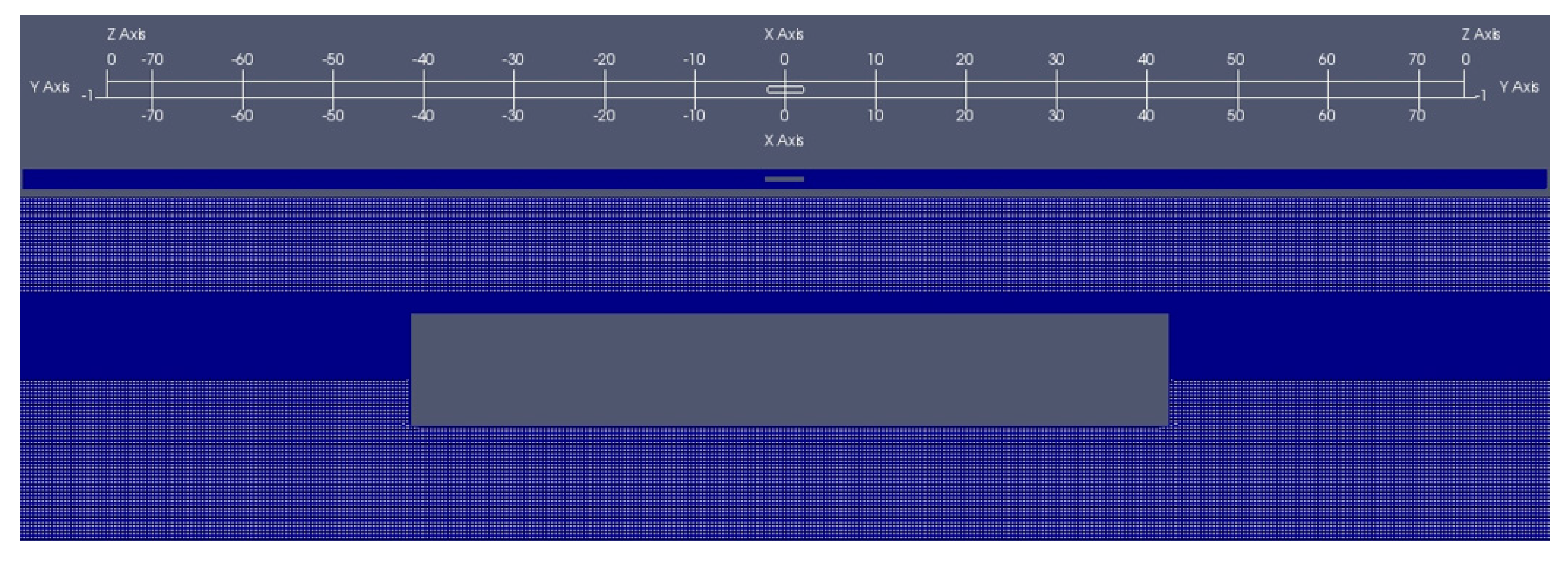
To run the CFD simulations, an open-source CFD toolkit, OpenFOAM, was used. OpenFOAM is an open-source library that numerically solves a wide range of problems in fluid dynamics from laminar to turbulent flows, with single and multi-phases. The solver has been elaborately described by [25]. The governing equations for the solver are the momentum or the Navier–Stokes equation for incompressible two-phase flow (18) and the continuity Equation (19). In vector form, the Navier–Stokes and continuity equations are given by:

$$\rho \left(\frac{\partial v}{\partial t}+v.\nabla v\right)=-\nabla p+\mu {\nabla }^{2}v+\rho g,$$

(18)

$$\nabla .v=0,$$

(19)

where $v$ is the velocity, $p$ is the pressure, $\mu$ is the dynamic viscosity, and $g$ is the acceleration due to gravity.

The volume of fluid (VOF) method is used to model the fluid as one continuum of mixed properties. This method determines the fraction of each fluid that exists in each cell, thus tracking the free surface elevation. The volume fraction is obtained by:

$$\frac{\partial \alpha }{\partial t}+\nabla .(\alpha v)=0$$

(20)

where $\alpha$ is the volume fraction of water in the cell, varying from 0 to 1, with 0 representing a cell full of air and 1 representing a cell full of water. The Finite Volume Method (FVM) is used to discretize the governing equations. Pressure–velocity coupling is obtained through the PIMPLE algorithm. The PIMPLE algorithm can be used to ensure multiple iterations between the flow parameters (outer correctors) to produce a stable and reliable solution without unwanted dissipation. An adaptive time-stepping approach was used to ensure a constant Courant–Friedrichs–Lewy (CFL) number during the simulation. All interpolation schemes in OpenFOAM, used for flux calculation in advection, operate with the MULES (Multidimensional Universal Limiter for Explicit Solution)-based solver. For convection (divergence) and diffusion terms, the Gauss linear Upwind and Gauss linear schemes are used.

To numerically reproduce the benchmark cases, simulations were run using OpenFOAM version 2.4.0 (https://openfoam.org/version/2-4-0/), together with waves2Foam in [26] module for wave generation. For solitary wave generation, the solitary wave model from [27] was used within waves2Foam. All benchmark simulations were run in two dimensions, to follow the proposed case setup. Since the Reynolds number for the simulated cases is relatively low, the flow was assumed to be laminar, and therefore no turbulence model was considered. Several wave gauges were placed along the simulation domain to probe the wave elevation.

CFD Setup

The study involves a rectangular pontoon encountering a solitary wave in a two-dimensional (2D) wave flume. The case setup consists of a 150-m-long 2D wave flume with a constant still water depth of 1.0 m. The rectangular pontoon has a width of 4 m, a draft of 0.4 m and 0.2 m above water height. Two wave gauges are placed in the domain at positions x = −31.0 m and x = 26.5 m, assuming the box is located at the centre (x = 0) of the domain (as shown in Figure 2).

To replicate the study numerically, simulations were run using OpenFOAM version 2.4.0, together with the waves2Foam module and OceanWave3D for wave generation. For solitary wave generation, initially, the wave model described in ref. [27] was used from waves2Foam. The simulations were run using 2D static mesh, to follow the proposed case setup. The flow was assumed to be laminar, and no turbulence model was used, considering the relatively low Reynolds number involved. Several wave gauges were placed along the simulation domain to probe the wave elevation.

The mesh domain for the case was generated following the case setup. For the first case, using the waves2Foam (see [27]) solitary wave model, the blockMeshDict was used to generate the simulation domain, and a single layer of refinement was applied using toposetDict to ensure proper propagation of the incoming wave. Finally, snappyHexMesh was used to integrate the rectangular pontoon into the simulation domain. The total resolution of the mesh was 3.1 million, with a spacing of 0.005 m in horizontal and vertical directions, in the wave propagation area. The resolution represents 200 cells per meter height and width of the pontoon. In terms of the soliton, a minimum of 20 cells per wave height was maintained. Several wave gauges were placed along the wave propagation area in the simulation domain to observe the wave propagation. A general mesh assembly used for the simulations is shown in Figure 3. A sufficiently large simulation domain was generated to ensure that on reflection is observed from the outlet of the domain. The simulation was terminated after a steady free surface profile was observed after the interaction, which happened much earlier before the propagating wave could reach the outlet of the domain. A mesh dependency study for wave structure interaction was previously reported in [28], and thus was not repeated here.

3.2. OceanWave3D Model Description

Just like the Boussinesq-type equations, the Fully Nonlinear Potential Flow (FNPF) formulation used in the OceanWave3D (OW3D) is based on the incompressible NS equations with further assumptions of zero vorticity and zero viscosity. The equations of balance are solved for each point of the domain (3D), considering all the remaining linear and nonlinear terms of the obtained equation. Thus, the formulation handles more complex problems than Boussinesq models, but is less complex than CFD. The FNPF formulation is therefore very suitable for nonlinear gravity waves propagation, including shoaling, reflection and dispersion of waves, as long as the waves do not break or acquire vorticity. It is also considerably less time-consuming than CFD techniques.

Once the flow assumes a potential $\phi (x,z;t)$, such that $V=(u,w)=(\nabla \phi ,{\partial }_z\phi )$, where $x$ is the horizontal position and $\nabla =({\partial }_x,{\partial }_y)$ is the horizontal gradient operator, the kinematic and dynamic and kinematic boundary conditions at the free surface read:

$${\partial }_t\zeta =-\nabla \zeta .\nabla \overline{\phi }+\overline{w}(1+\nabla \zeta .\nabla \zeta ),$$

(21)

$${\partial }_t\overline{\phi }=-g\zeta -\frac{1}{2}\{\nabla \overline{\phi }.\nabla \overline{\phi }-{\overline{w}}^2(1+\nabla \zeta .\nabla \zeta )\},$$

(22)

where $\zeta$ and $g$ are the same as defined in Section 3.1. The boundary conditions at the free surface and sea bottom read:

$$\phi =\overline{\phi }\mathrm{for}z=\zeta ,$$

(23)

$${\partial }_z\phi =-\nabla h.\nabla \phi \mathrm{at}z=-h,$$

(24)

and the Hamilton equation reads as:

$${\nabla }^2\phi +{\partial }_{zz}\phi =0\mathrm{for}-h<z<\zeta .$$

(25)

For further details on the numerical scheme used to solve this nonlinear problem, the reader is referred to [29].

A coupled OW3D and OpenFOAM module is used to propagate the solitons over a fixed depth and simulate the interaction between a soliton and a fixed pontoon for varying soliton amplitudes. However, the solitons must be generated before being propagated. For that, the MATLAB^® code presented in [30] was considered. It is important to mention that the FNPF one soliton propagating stably over fixed depth may be defined by: (1) water depth and soliton’s amplitude or, (2) water depth and soliton celerity’s. In non-dimensional values, a soliton may be simply defined by a single parameter, which may be the non-dimensional soliton amplitude $(a/h)$ or the Froude-depth number $(F_n=c/\sqrt{gh})$.

OceanWave3D Setup

As for OceanWave3D, the coupling of the OW3D domain to that of the OpenFOAM happens at the inlet and the outlet of the OpenFOAM mesh domain. The inlet velocity boundary of the mesh domain is set to the waveVelocity received from the OW3D domain. The outlet boundary is also set to waveVelocity, which transfers the outward wave back to the OW3D domain. As before, the simulation solver is waveFoam, which solves static mesh with waves. The mesh was generated with blockMeshDict and snappyHexMesh, without any refinement. The total resolution used in the mesh was around 1.3 million, with grid size in the horizontal and vertical direction being 0.005 m and 0.005 m, respectively. The average time step size was 0.007 (s). The general mesh assembly used in the simulation is shown in Figure 4. Unlike the previous case, here, instead of placing the pontoon at $x=0$, the pontoon was placed at $x=100$. This was done to accommodate the OW3D domain, which starts at $x=0$. The OW3D domain was larger by 50 m on each side (x-axis) to ensure the entry of a stable soliton at the inlet and no reflection from the outlet after solitary wave leaves the OpenFOAM domain after interaction.

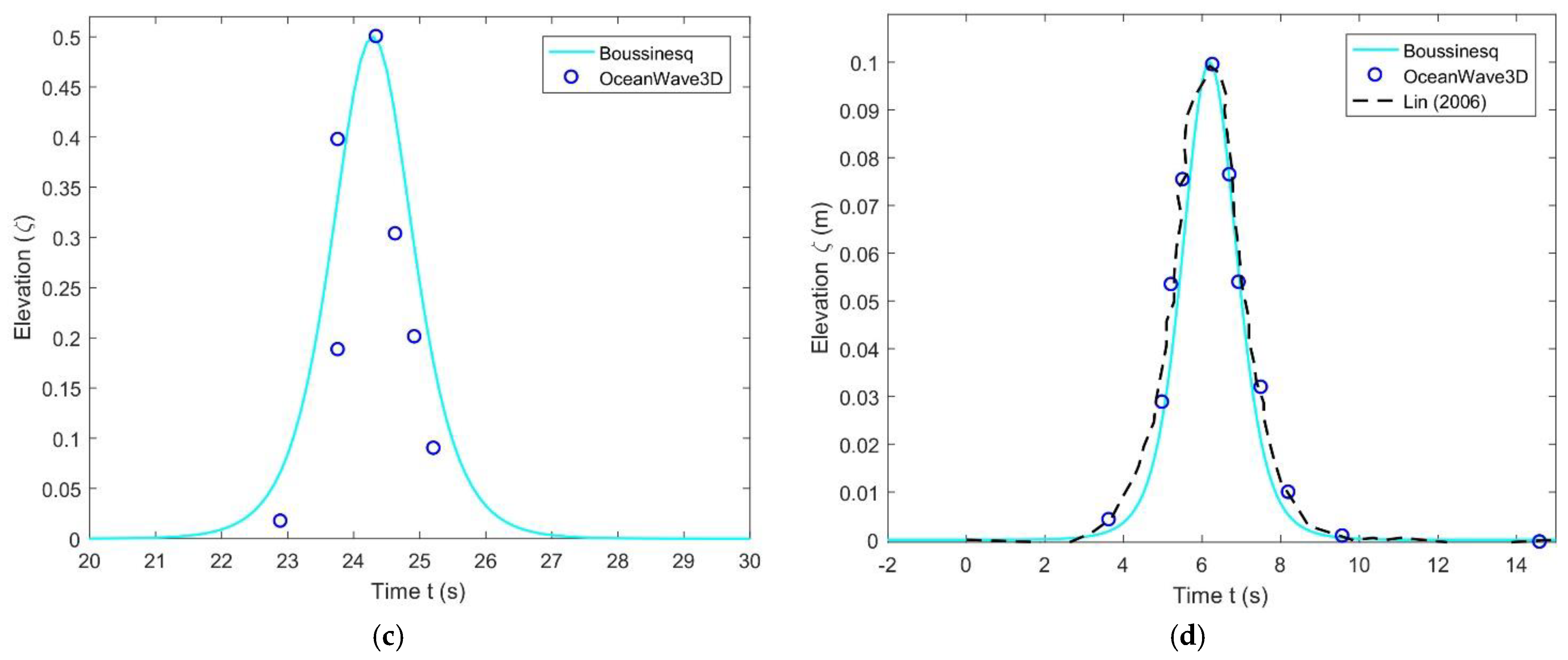
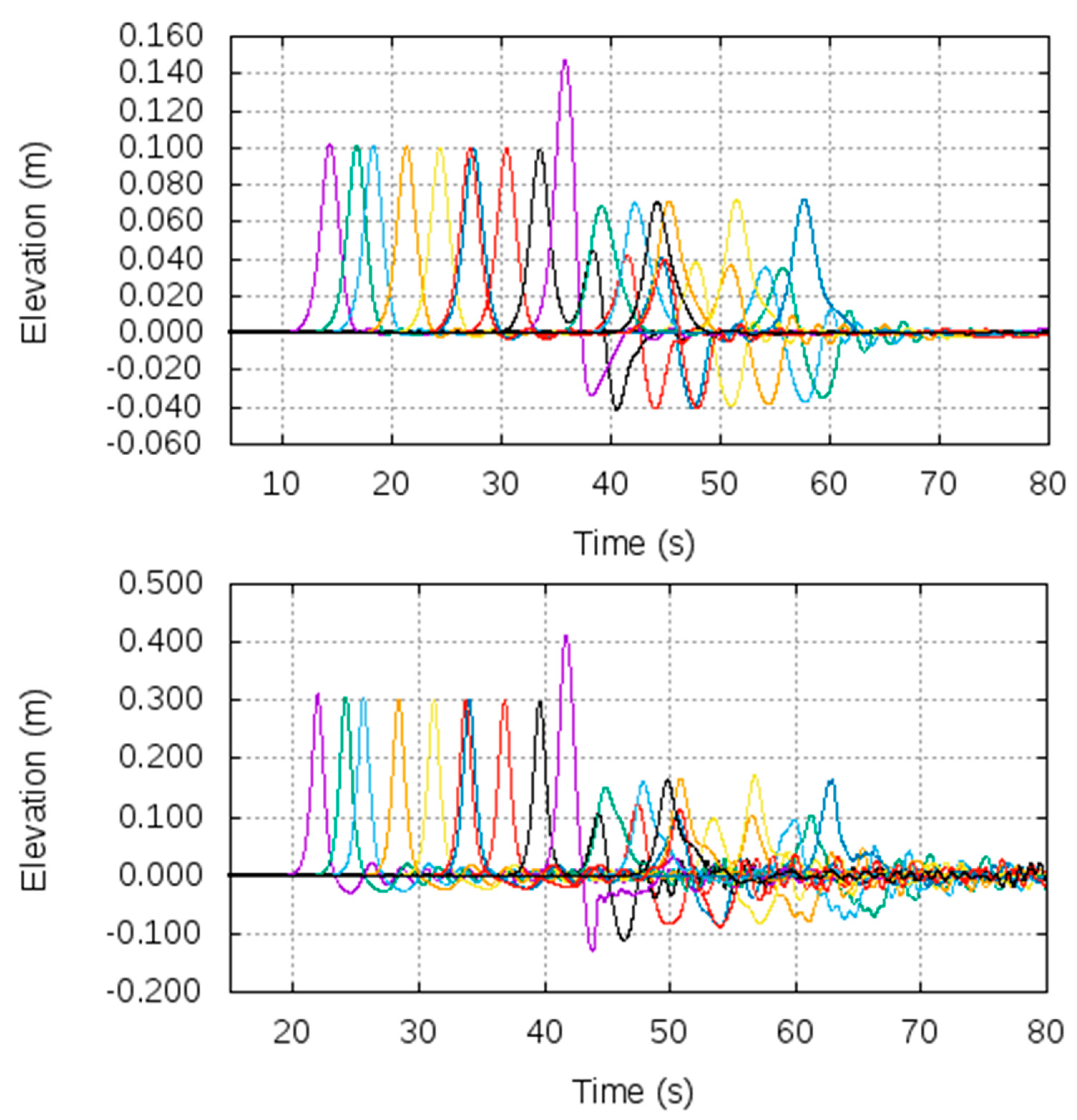
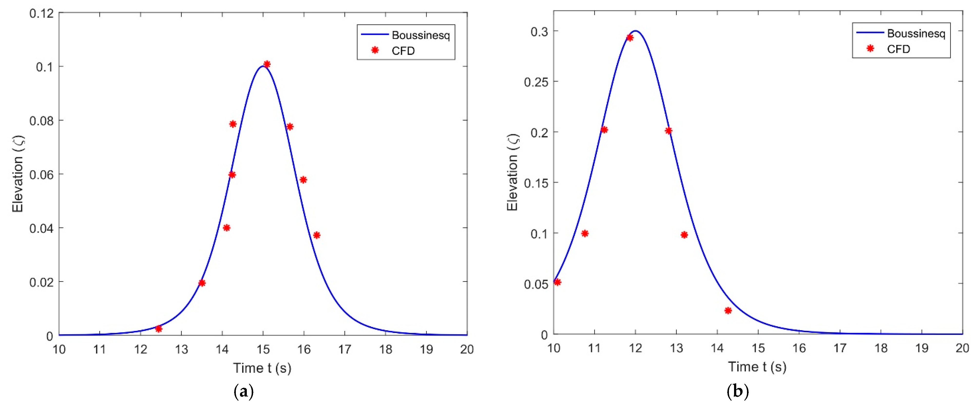
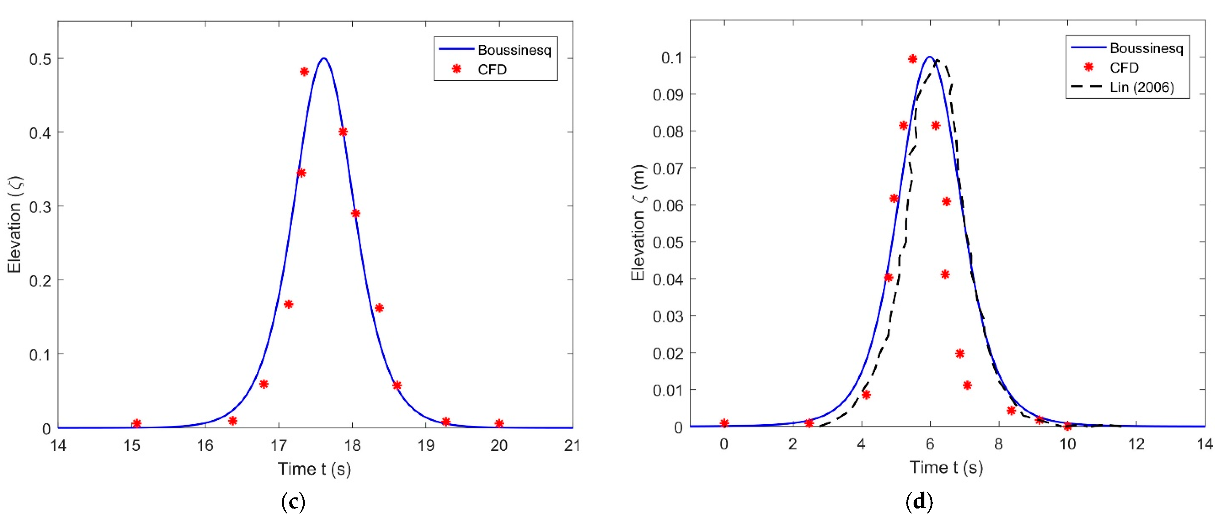
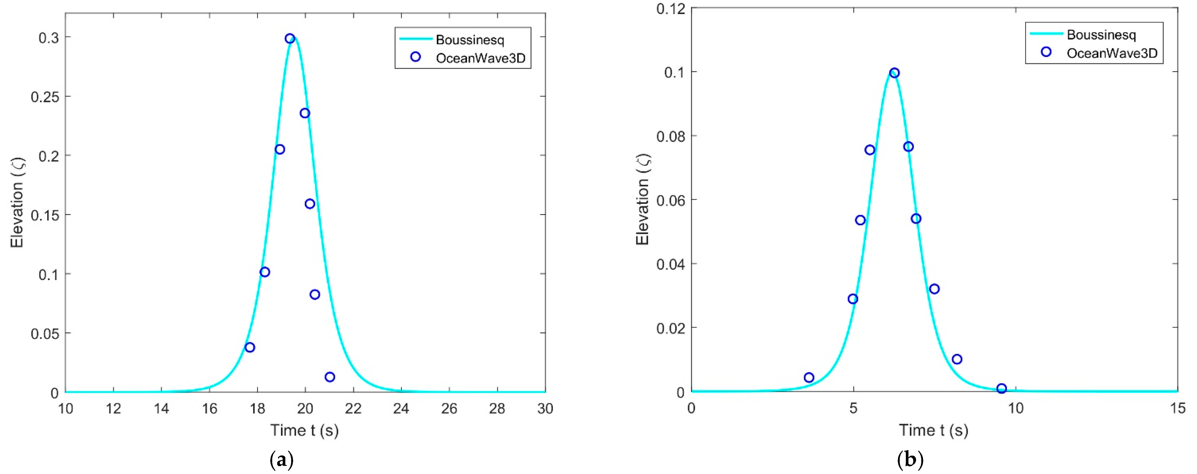
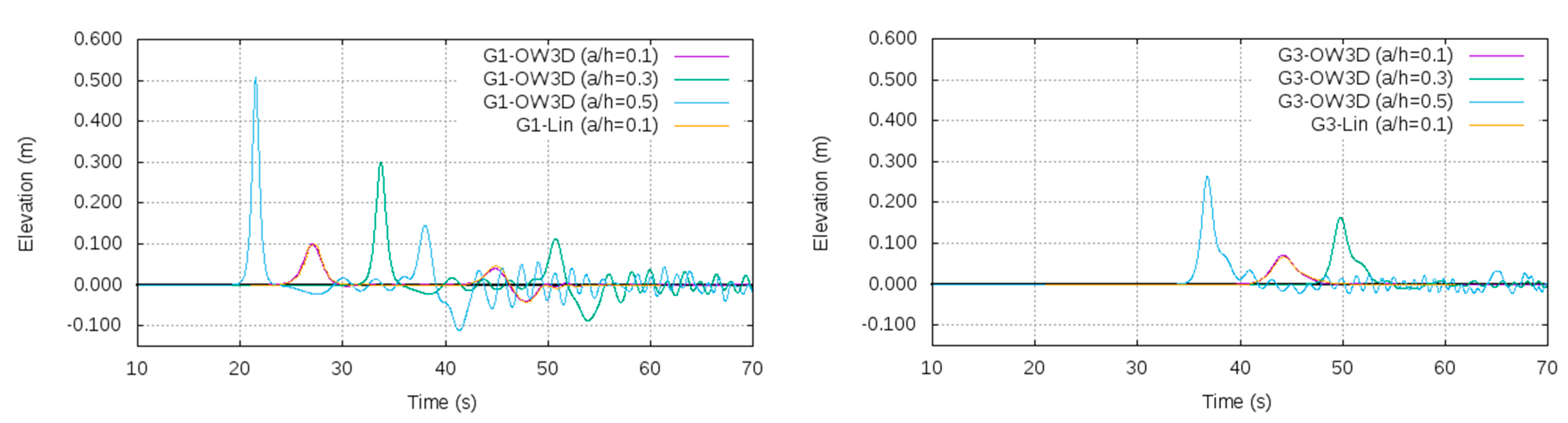
4. Comparison of Wave Elevation from Different Models

Figure 5 shows comparisons of the solitary waveform $\zeta (\mathrm{m})$ in the outer region against CFD model simulations for different nonlinear quantities $(a)\epsilon =0.1,\left(\mathrm{b}\right)\epsilon =0.3,\mathrm{and}(c)\epsilon =0.5$ and (d) their comparison with an external numerical model (see [31]) versus time t (s). From Figure 5a,b, it can be observed that the peak amplitude of the solitary wave is in good agreement, and the solitary wave profile trend is similar to the CFD model results. However, the peak amplitude for $\epsilon =0.5$ CFD is higher than that of analytical results, but the trend is similar. The discrepancy in the results between the analytical and CFD simulations may be due to the consideration of second-order approximation in analytical and full nonlinear in the CFD model. Figure 5d shows that the analytical solitary wave profile is very close to the CFD and EFD model simulations. Further, in Figure 5c, the peak amplitude of the solitary wave from the analytical model is 0.5 m, while the CFD model is 0.56 m, which is 6% larger. However, the agreement of solitary wave profiles between analytical and CFD is almost 95%.

Figure 6 compares the results of a solitary wave from analytical and OceanWave3D model simulations in the outer region for different degrees of nonlinearity $(a)\epsilon =0.1,\left(\mathrm{b}\right)\epsilon =0.3,\mathrm{and}(c)\epsilon =0.5$ versus time t (s). In this case, it can be seen that the peak amplitudes between analytical and OceanWave3D results are in good agreement, and their profiles also show a similar trend. However, in Figure 6c there is a small discrepancy in their trends, maybe for a similar reason to that described in Figure 5.

In Figure 6a–c, it is shown that the agreement of peak amplitude of the solitary waves between analytical and OceanWave3D is about 97%. On the other hand, Figure 6d demonstrates that the solitary wave profile between analytical, OceanWave3D, and Numerical model (NM) from other calculations (see [31]) are in good agreement.

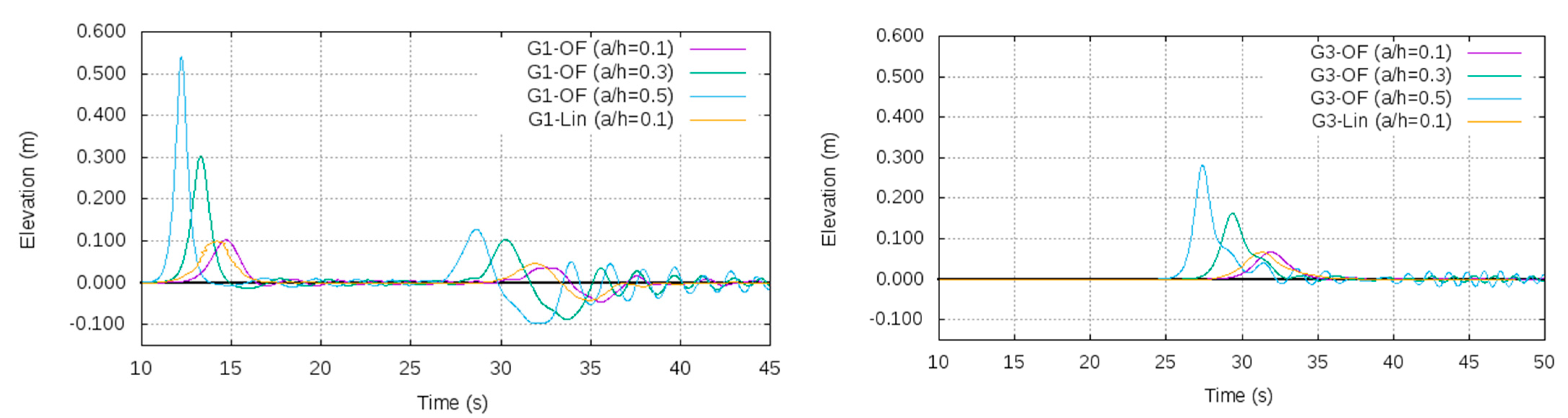
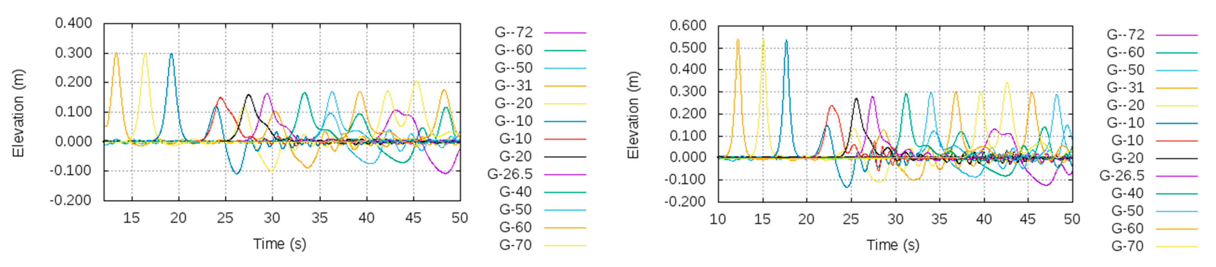
5. Analysis of Results from CFD, OceanWave3D, and Analytical Model Simulations

In this section, the effect on the wave forces and pressure distributions around the pontoon for different $\epsilon =a/h$ is analysed based on the CFD and OceanWave3D model simulations. Further, the effect of the Ursell number, pontoon length, and water depth on the solitary wave profiles are analysed based on the analytical solution. In the CFD study, six simulations are performed in total, with three different solitary wave amplitudes, using two different wave generation formulations. For initial validation of the results, simulations were performed for the non-dimensional solitary wave amplitude, $a/h=0.1$(0.1 m) and compared with the results of [31]. Later, two more cases are simulated using the amplitude of 0.3 m $(a/h=0.3)$ and 0.5 m $(a/h=0.5)$.

The intention is to assess the effectiveness of a pontoon type wave breaker against solitary waves of different steepness. It may be mentioned that no experimental data are available for the case; however, several numerical studies have been performed previously with VOF-RANS (see [31]), σ-transformed NS (see [31]) and layer-averaged RANS (see [32]).

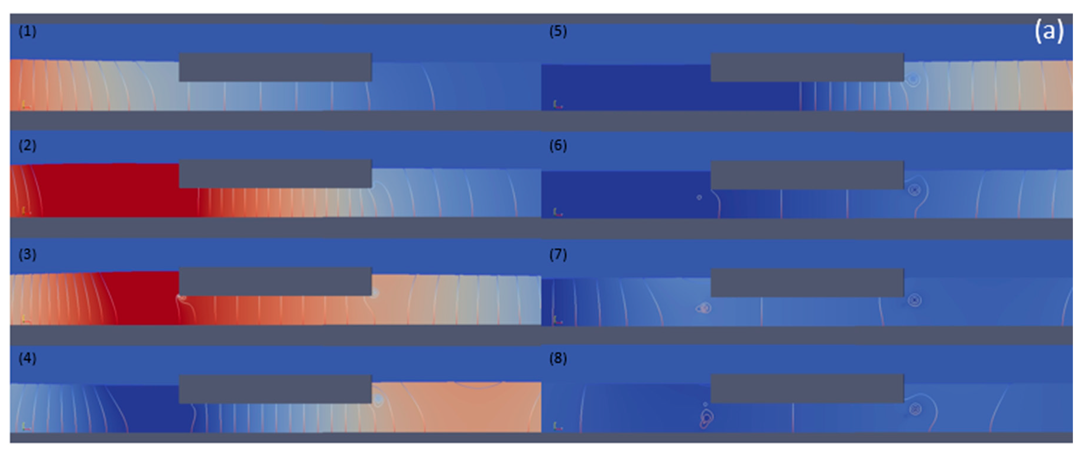
5.1. Solitary Waveform Generated Using the Chappelear Model (Waves2Foam)

The Chappelear model (see [30]) is a second-order solitary wave generation model that is used to generate and propagate the solitary wave in the domain. Initially, simulation is performed with amplitude 0.1 m so that the results can be compared with available data. During the simulation, wave elevations are measured at different positions of the domain. Measurements from all the gauges are shown in Figure 7. The gauge numbers indicate the location of the gauge in the domain. The results show that after interacting with the fixed pontoon, a portion of the solitary wave advances, while a reflected wave propagates backwards. The forwarding soliton propagates with roughly 0.06 m amplitude after the interaction. Meanwhile, the reflected wave propagates backwards with a crest and a trough of roughly 0.04 m.

Figure 8 shows a relative comparison among the previous numerical results (see [31]) and the present simulation results for wave gauges G1 and G3. The figure shows simulation results for $a/h=0.1,0.3,\mathrm{and}0.5$, whereas Lin (see [31]) only presented results for $a/h=0.1$. The timeline for the numerical study from Lin (see [31]) also differs from the simulation timeline of OpenFOAM, so the time values (x-axis) were shifted to bring the curves closer. A difference of 10 s was observed for soliton propagation comparing to Lin [26]. The difference most probably come from the wave initiation time and position, which might have varied for the two solutions. Generally, in RANS simulations, a time delay is applied on wave generation and propagation to ensre better simulation stability.

From the simulations, wave elevation at gauge G1 and G3 are measured. The figure shows that the wave model generates the soliton with the right wave amplitude (gauge G1, at −31 m) of steepness 0.1. The figure shows good agreement among the results for steepness 0.1, for both the propagating soliton and the reflected waves. As for the amplitude of the propagating wave after interaction with the pontoon (gauge G3, at 26.5 m), the simulation results show slight over-prediction compared to previous numerical predictions. Nevertheless, the presented simulation results in Figure 5 show a good agreement with previous numerical data.

The results from the wave gauges (Figure 7) show that the soliton shows a dispersive tail during propagation and as a result, the free surface shows slight oscillation. This dispersive tail reduced the soliton energy slightly, causing its amplitude to reduce, over the period of propagation. The dispersive tail is not observed in the numerical results of [31], which might be due to the simplified assumptions for wave modelling. Experimental studies performed with solitary waves also show dispersive tail in the channel (as in [30]), which confirms that the observed scenario in the simulation is not unphysical.

The horizontal and vertical forces encountered in the pontoon are also measured during the wave encounters, and the results are shown in Figure 9 and Figure 10. The forces are important for understanding the mooring force required to hold the pontoon in place or for studying the feasibility of installing a wave energy converter for dual purposes. However, the pontoon studied in this paper is fixed, and no mooring lines are used in the simulations. While inclusion of mooring lines would surely affect the forces and moments, the static results still provide a reference regarding the required mooring line properties.

The high-frequency oscillations observed in force come from the overtopping of water on the pontoon. After the solitary wave interacts with the fixed pontoon, for the $a/h=0.3$ and 0.5 cases, wave overtopping occurs. As such, the force–time history is the summation of forces on top of the pontoon and below it. The oscillating part comes from the integrated force on top of the pontoon that comes from the overtopped water.

As expected, the force results show a gradual increase in surge and heave forces with increasing amplitude of the soliton. The heave force encountered by the pontoon is substantially larger compared to the encountered surge force. For the high amplitude cases, the pontoon encounters almost the same level of positive and negative heave force while encountering the solitary wave. The time stamp on the force history also provides a relative idea regarding the propagation velocity of the solitary waves. As expected, high amplitude waves propagate faster compared to low amplitude waves. The propagation velocity is also affected by the vertical steepness of the propagation area (see [4]). The pitch moment is also of high interest for soliton–pontoon interaction, since it is generated from localized pressure on certain section of the pontoon, which in turn creates a high overturning moment. In fact, refs. [11,33,34] demonstrated that the pitch moment in such cases is high enough to over-stress the structural components and connections. Thus, the pitch moment predicted from the simulations is also shown in Figure 11. The results show that the pontoon experiences a sharp rise in pitch moment after a certain period of interaction.

In Figure 12, pressure distribution in the flow field close to the pontoon is shown. The figure better illustrates the wave interaction with the static pontoon. Pressure distribution in the fluid domain is shown for the cases with amplitude 0.1 m, 0.3 m, and 0.5 m in Figure 12a–c. Figure 12 shows the solitary wave breaking part and shows the interaction of the wave with the fixed pontoon. While Figure 12 shows the sequence of interaction, the other two cases show simulation time. Overtopping of the wave is observed for amplitudes 0.3 m and 0.5 m. For all three cases, small eddies or vortices are observed at the sharp ends of the pontoons. All three images use a different pressure scale, since the aim is to present the wave interaction and not to measure the encountered pressure.

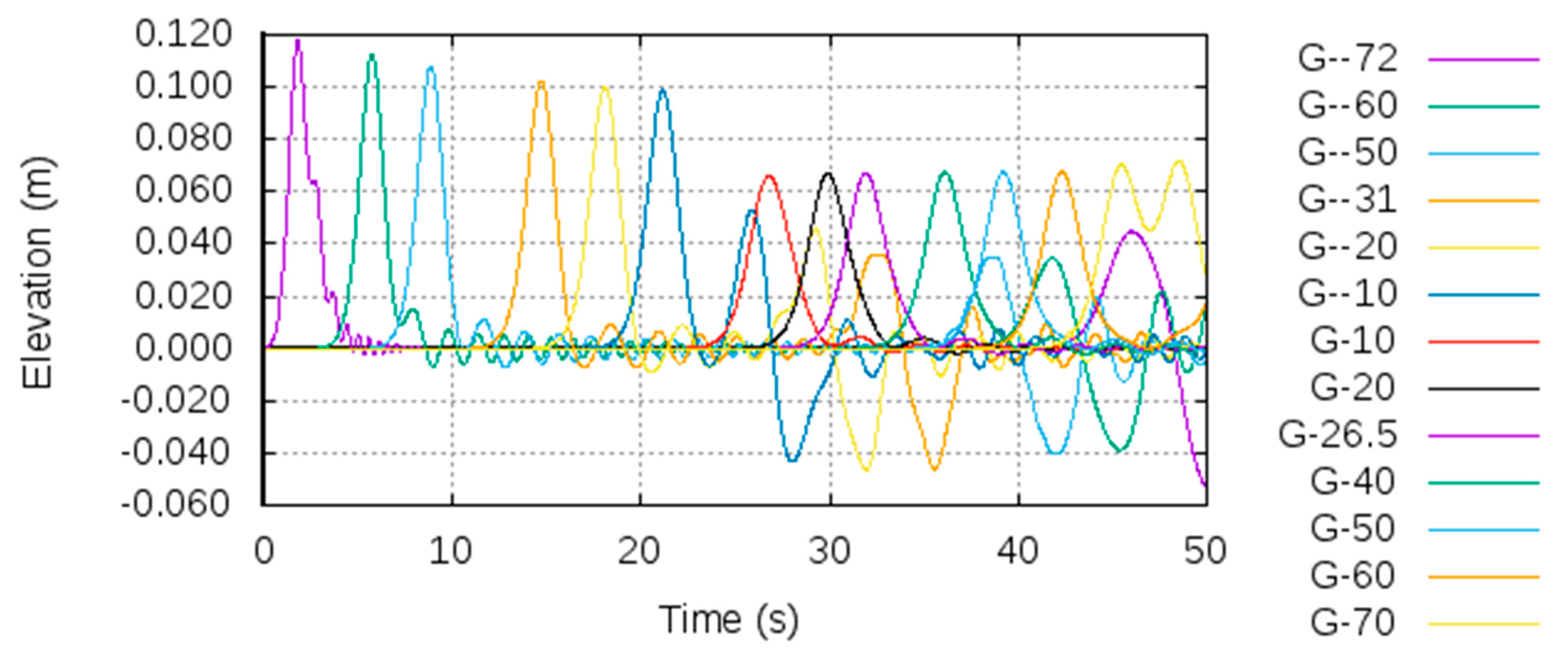
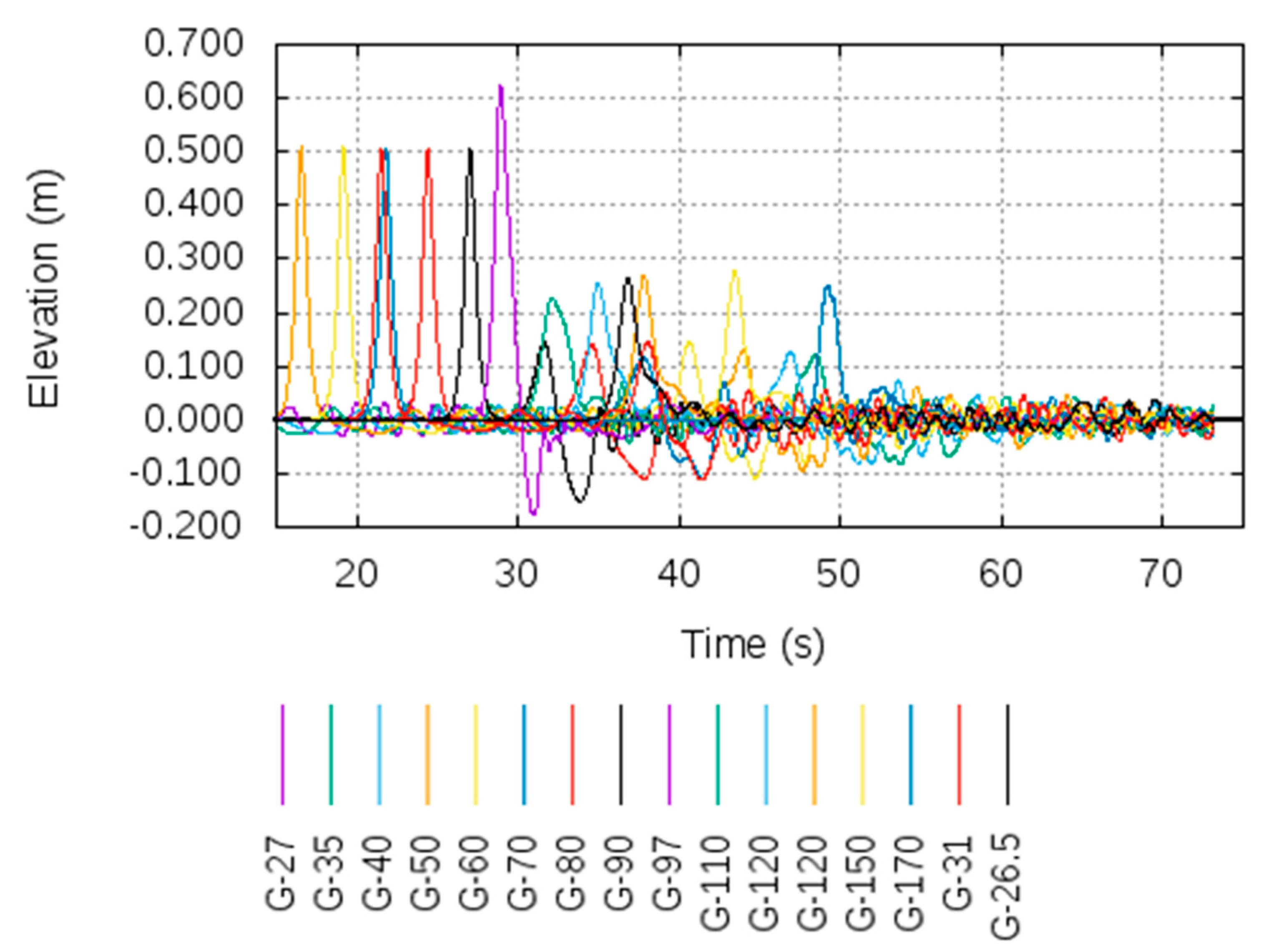
5.2. Solitons Generated Using the OceanWave3D Model

Next, simulations are performed using a coupled model between OpenFOAM and OceanWave3D (OW3D), a Fully Nonlinear Potential Flow (FNPF) code by [29]. The solitons are generated by inputting the exact wave flux of an FNPF soliton solution obtained from the conformal mapping technique in [30]. Initially, the solitons are simulated on OW3D separately to check for the stability of the solution. After checking the stability of the soliton, the input parameters are used in the coupled model. In theory, solitons propagating over fixed depth are stable up to the limit of around $a/h=0.76$.

As before, initially, simulation is performed with the amplitude of 0.1 m (a/h = 0.1) and compared with the available numerical data, as shown in Figure 5. Compared to Figure 5, the results show improvement in measured wave elevations. The presented CFD results, coupled with the OW3D model, show better agreement with previous numerical results compared to the Chappelear wave model (see [27]).

The wave elevations measured by all the wave gauges (for $a/h=0.1,0.3,\mathrm{and}0.5$) are shown in Figure 12. The respective numbers after the G here indicate the position of the gauge in the domain. G-31 and G-26.5 represent G1 and G3 in the original setup. They are represented as G-31 and G-26.5, instead of being referred to by their actual position in the domain, to avoid confusion.

When compared with Figure 7 (for a/h = 0.1), Figure 13 shows more stable wave propagation and negligible dispersive tail after the soliton. This is most probably linked to the viscosity effect, which is not well captured in the coupled model, hence the deviation from the experimental observation. Furthermore, due to the positioning of the wave probes, the simulation was also able to capture the peak of the solitary wave before breaking, as shown by gauge 97. However, OW3D shows a loss of wave amplitude by 30%, in contrast to the second-order Chappelear model (see [27]), which showed a 35% loss. This can be related to the stable propagation of the solitary wave without dispersive tail, which causes loss of energy.

As for $a/h=0.3$ and $a/h=0.5$, similar to the previous case, due to the positioning of the wave probes, the probe placed at position 97 captures the peak of the soliton before breaking. Furthermore, the Figures suggest, for higher amplitude cases, the soliton generated by OW3D also shows a dispersive tail. Nevertheless, the generated solitons using OW3D are more stable and does not lose amplitude before interacting with the pontoon. According to the figures after the interaction, the soliton propagates with an amplitude of 0.068 m. Whereas, the reflected wave propagates backwards with a crest and trough of roughly 0.04 m amplitude.

As before, a comparison is shown in Figure 14 among the CFD results for G1 and G3 wave gauges $a/h=0.1,0.3,\mathrm{and}0.5$, and the results from [31] at a/h = 0.1. The comparison among a/h = 0.1 results shows good agreement. Like the previous case, the time for the Lin results (see [31]) is also adjusted here for overlapping. In the case of OW3D results, the $a/h=0.1$ case shows wave propagation in between the 0.3 and 0.5 cases. This is because the domain sizes for the $a/h=0.3$ and 0.5 cases are different from the 0.1 cases. The domain configuration had to be changed to create a stable solitary wave with the right amplitude. Thus, they show different times of interaction.

Next, a relative comparison among the surge and heave forces experienced for different wave amplitudes is shown in Figure 15 and Figure 16. For all the cases, the surge force results show a slight underprediction, compared to the Chappelear model ([27], non-coupled solution), in predicting the positive force, while they slightly overpredict the negative force. As for the heave force, the results show minor overprediction of positive forces compared to the Chappelear model (see [27]), whereas negative forces show a notable underprediction. This difference might be partly due to the difference in mesh resolution. However, the major difference should be a result of the difference between the two models.

Finally, pressure distribution in the flow field close to the pontoon is shown for all three cases in Figure 17. Pressure distribution is shown for the cases with amplitude 0.1 m, 0.3 m, and 0.5 m in Figure 17a–c, respectively. As before, overtopping of a wave is observed for amplitudes of 0.3 m and 0.5 m. However, for the coupled simulation, the small eddies or vortices are less visible below the pontoon. The images here use a different pressure scale, as well, since the same scale comparison will not be sufficient to show the slight gradients in pressure during the encounter.

Overall, it may be concluded that both the Chappelear (see [27]) and coupled OW3D models show similar predictions, and both might be used for studying floating body interaction with a solitary wave. However, the solitary wave generated using OW3D shows better stability compared to the Chappelear model present in waves2Foam. Furthermore, OW3D coupled simulations showed significantly shorter run-time (20 h) compared to the Chappelear model in waves2Foam (100 h). Considering the computational cost and relative accuracy, the OW3D coupled model seems more practical for such studies. The numerical computations associated with analytical expressions were performed in a desktop machine with Intel^® core i7-4790 CPU with a 3.60 GHz processor and 32 GB of RAM. On average, each case took roughly 10–15 min to finish.

5.3. Behavior of Solitary Waves Based on Analytical Solution

In this subsection, the effect of different parameters, such as the Ursell number, plate length, and water depth on the behaviour of the solitary wave is analysed based on the analytical solution. To start, Figure 18 shows the effect of solitary wave profiles in the outer region for different Ursell numbers versus water plane length x (m). It can be clearly seen that, as the Ursell number increases, the solitary wave profile $\zeta$ compresses, having the same peak for each Ursell number.

In Figure 19, the effect of solitary wave profiles in the outer region for different pontoon lengths versus water plane length x (m) is plotted. It can be observed that, as the length of the pontoon increases, the solitary wave shifts towards the right, while maintaining similar wave amplitude throughout the water plane length. A certain shifting to right in the solitary wave profiles is observed which is due to the constructive/destructive interference of the incident and reflected waves at the edge of the structure.

Figure 20 shows the variation in solitary wave profiles for different water depths versus x (m). It can be seen that the effect of water depth on the solitary wave profiles is insignificant. However, it caused a small effect at the bottom of the solitary waves, but not at the peak.

5.4. Wave Energy Analysis

Finally, energy analysis is performed on the OpenFOAM CFD results to calculate the loss of energy of the solitary wave after interaction with the pontoon. The energy calculation is performed based on the incident and transmitted solitary wave amplitudes, and the energy formulation for exact solitary solutions. However, the energy of the reflected wave is not calculated. To perform the calculation, soliton amplitudes are recorded from the wave gauges used in the simulation domain, as shown in Figure 7 and Figure 21. For the propagating wave after the interaction, the stable average amplitude is considered. As can be seen from the figure in the case of a/h = 0.5, the soliton breaks after propagating forward.

The energy analysis results are shown in

Table 1. Energy analysis results for the solitary wave interacting with a fixed pontoon.

Amplitude (a/h)	Input Energy (J)	Transmitted Energy (J)	Loss of Energy after Interaction	Loss of Amplitude after Interaction
0.1	5.10 × 10−2	2.76 × 10−2	46%	33%
0.3	2.82 × 10−1	1.23 × 10−1	57%	41%
0.5	6.87 × 10−1	2.71 × 10−1	60%	45%

. The table shows that the higher the initial amplitude, the higher the loss of solitary energy. In addition, energy is being reflected, absorbed, and dissipated. The dissipation of energy also increases with initial amplitude, which can be observed in Figure 7 and Figure 21, which show longer dispersive tails for higher-amplitude cases.

6. Conclusions

This paper presents a new mathematical model, which is the Boussinesq formulation and solitary wave solution. Moreover, the application of the technique to the considered problem is new, and the comparison with two different independent numerical model simulations and its analysis are also new. Furthermore, the coupled numerical model between CFD and OceanWave 3D is another new contribution of the present study. The solitary waves are generated using 2nd-order solitary wave theory and a coupled FNPF model. The analytical solitary wave is compared with CFD and OceanWave3D (FNPF) model simulations for three-different soliton amplitudes. The solitary wave solution in the outer region associated with the aforesaid model is derived and comparison results with two different higher-fidelity numerical models are presented. From the present study, it can be concluded that:

• The compared results of the analytical model showed that the solitary waveform in the outer region is very close to CFD, OceanWave3D, and previous numerical results from the literature.
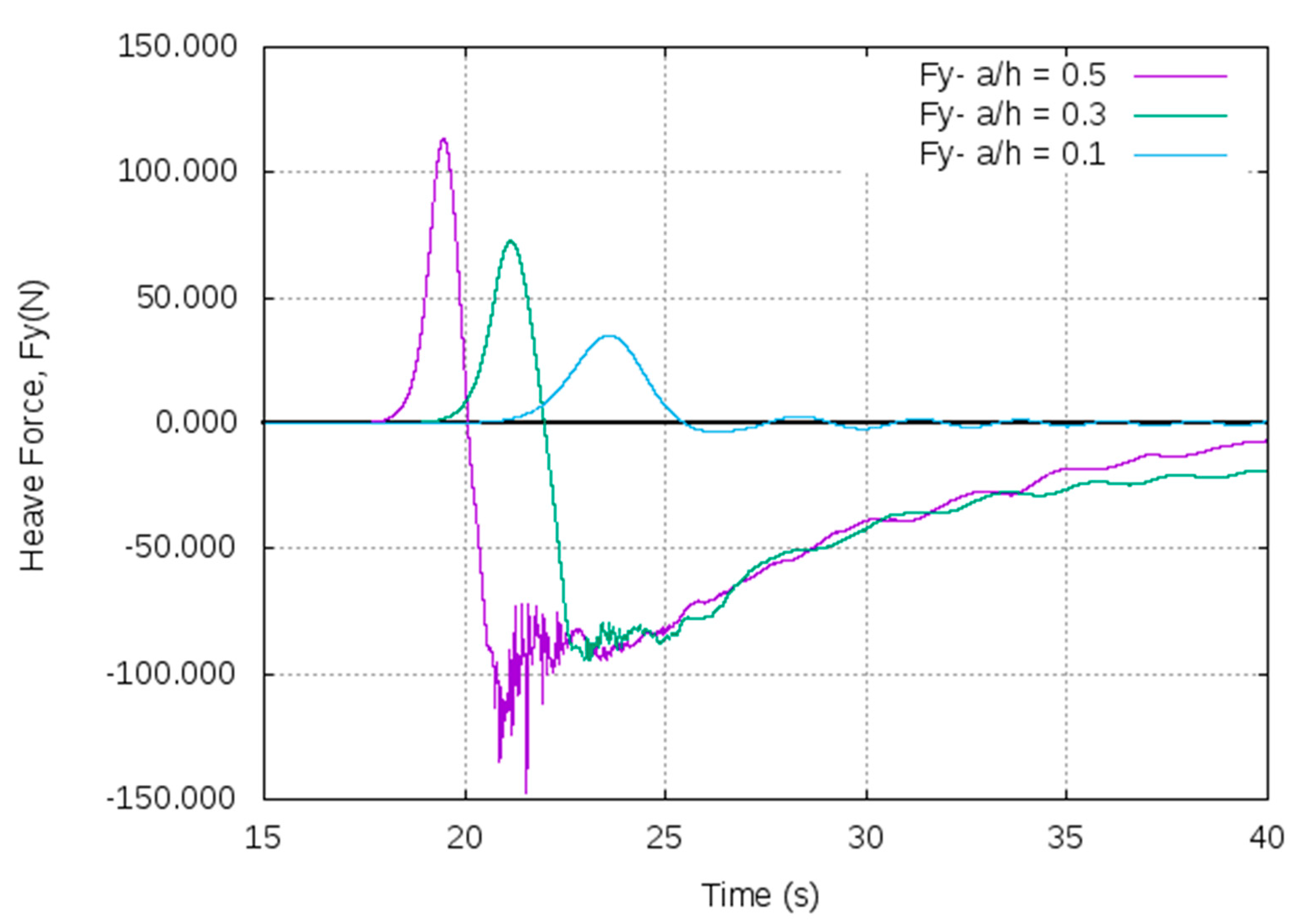
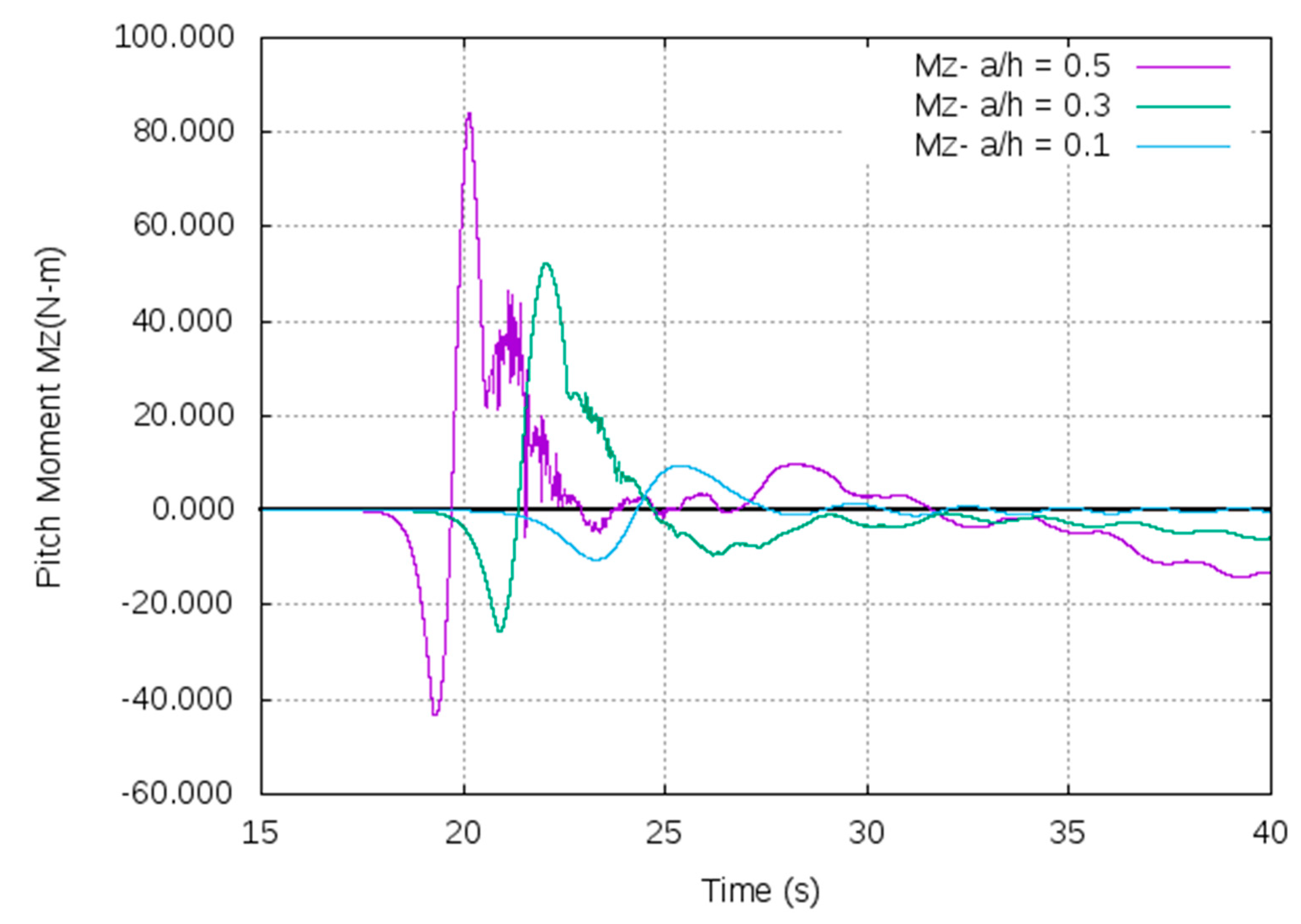
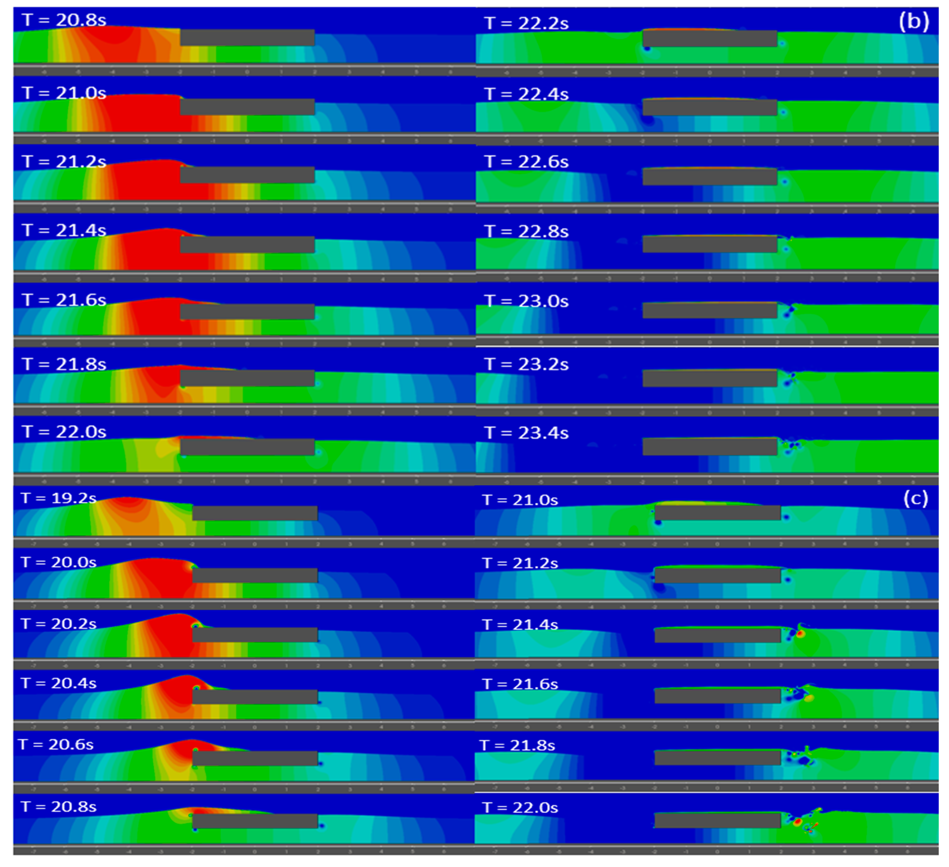
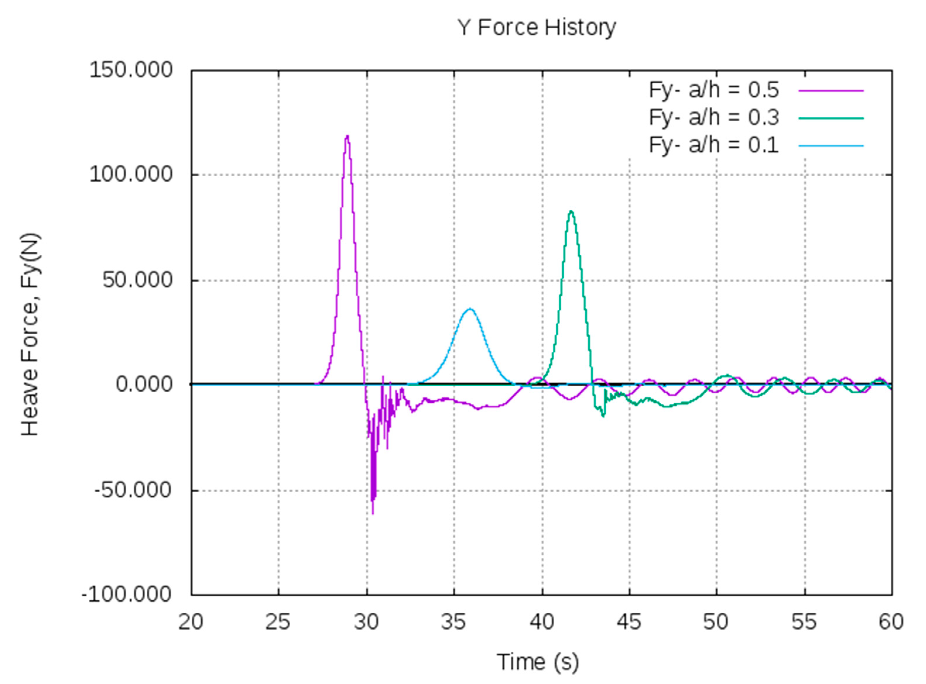
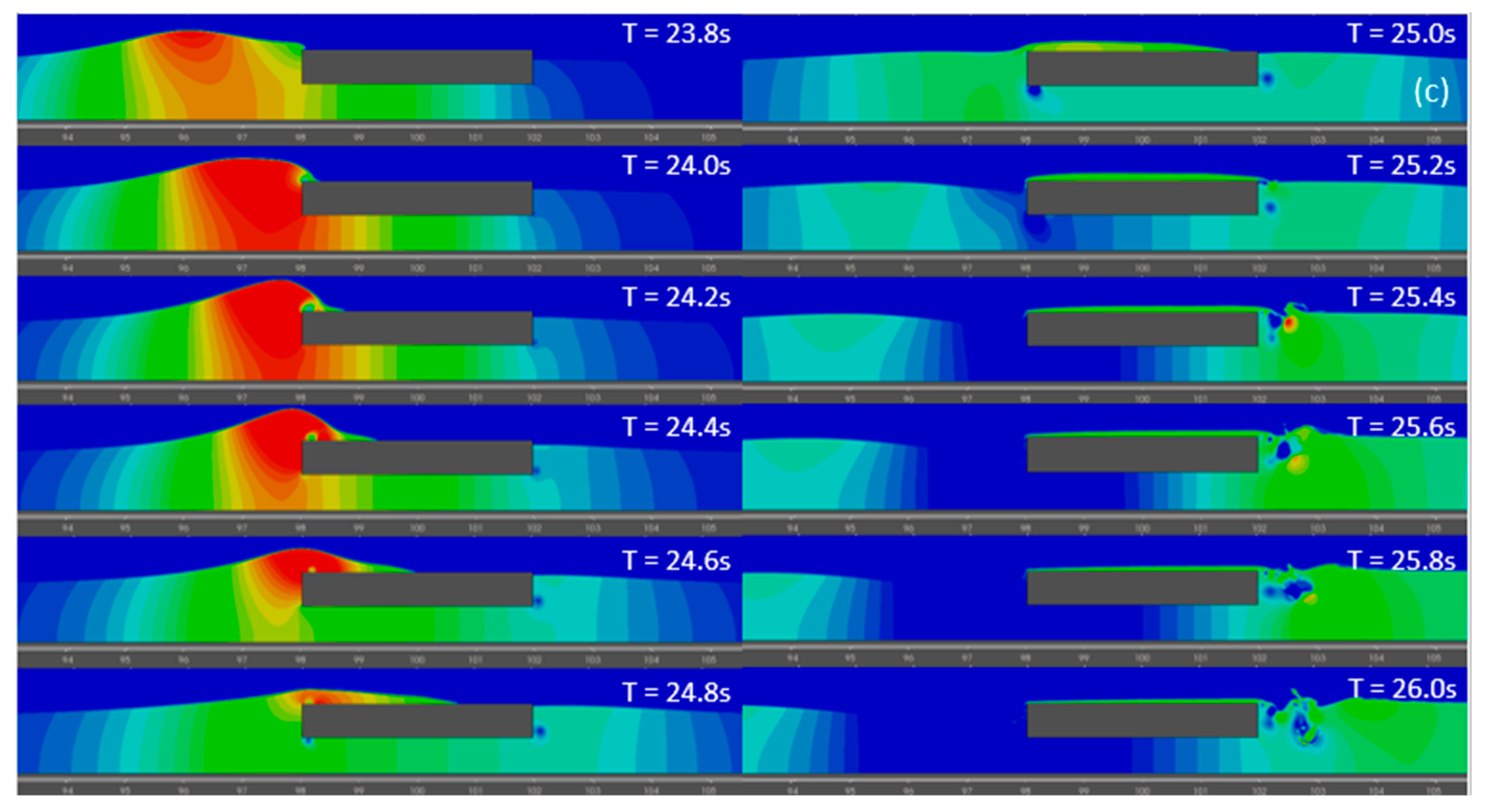
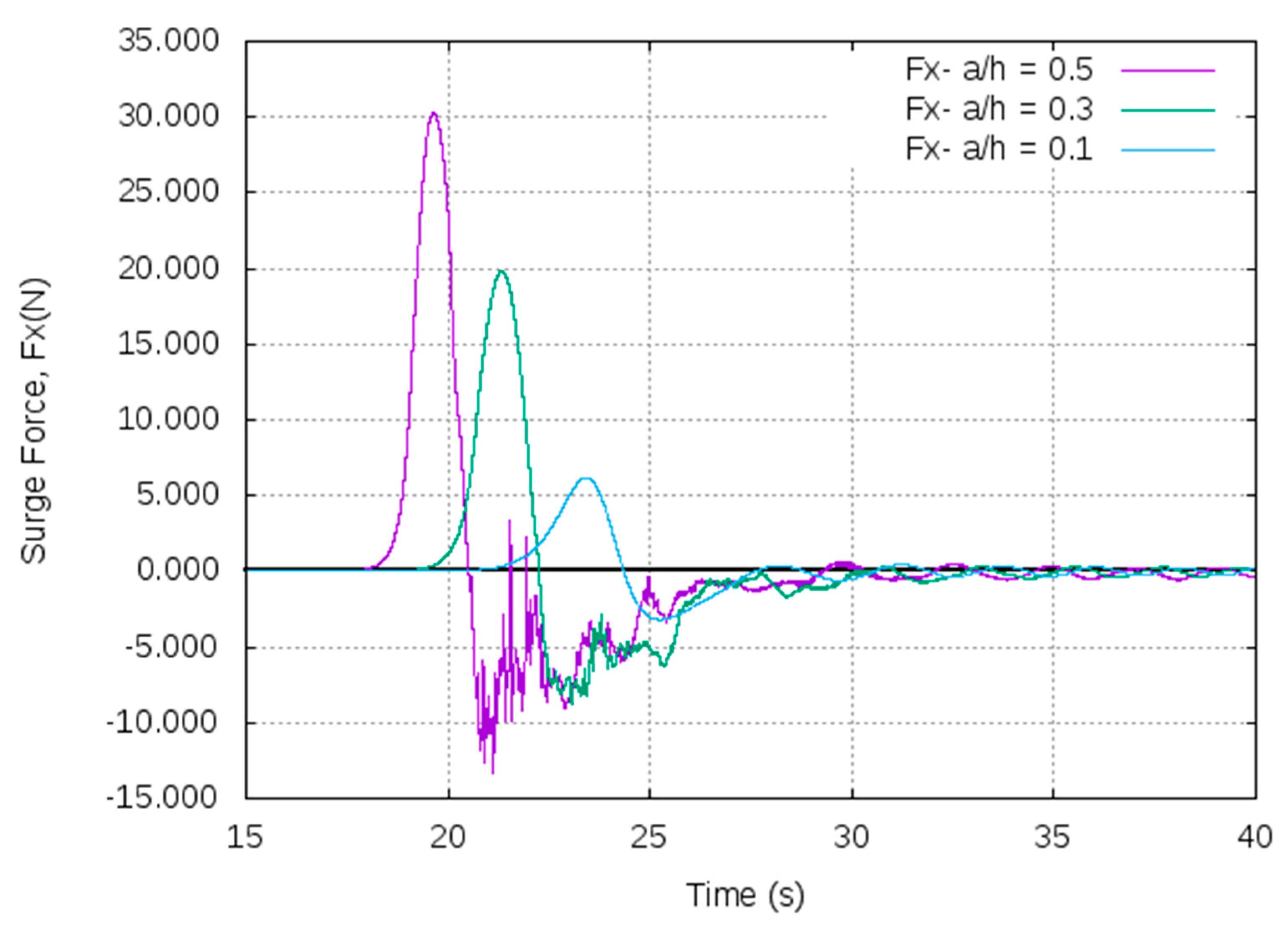
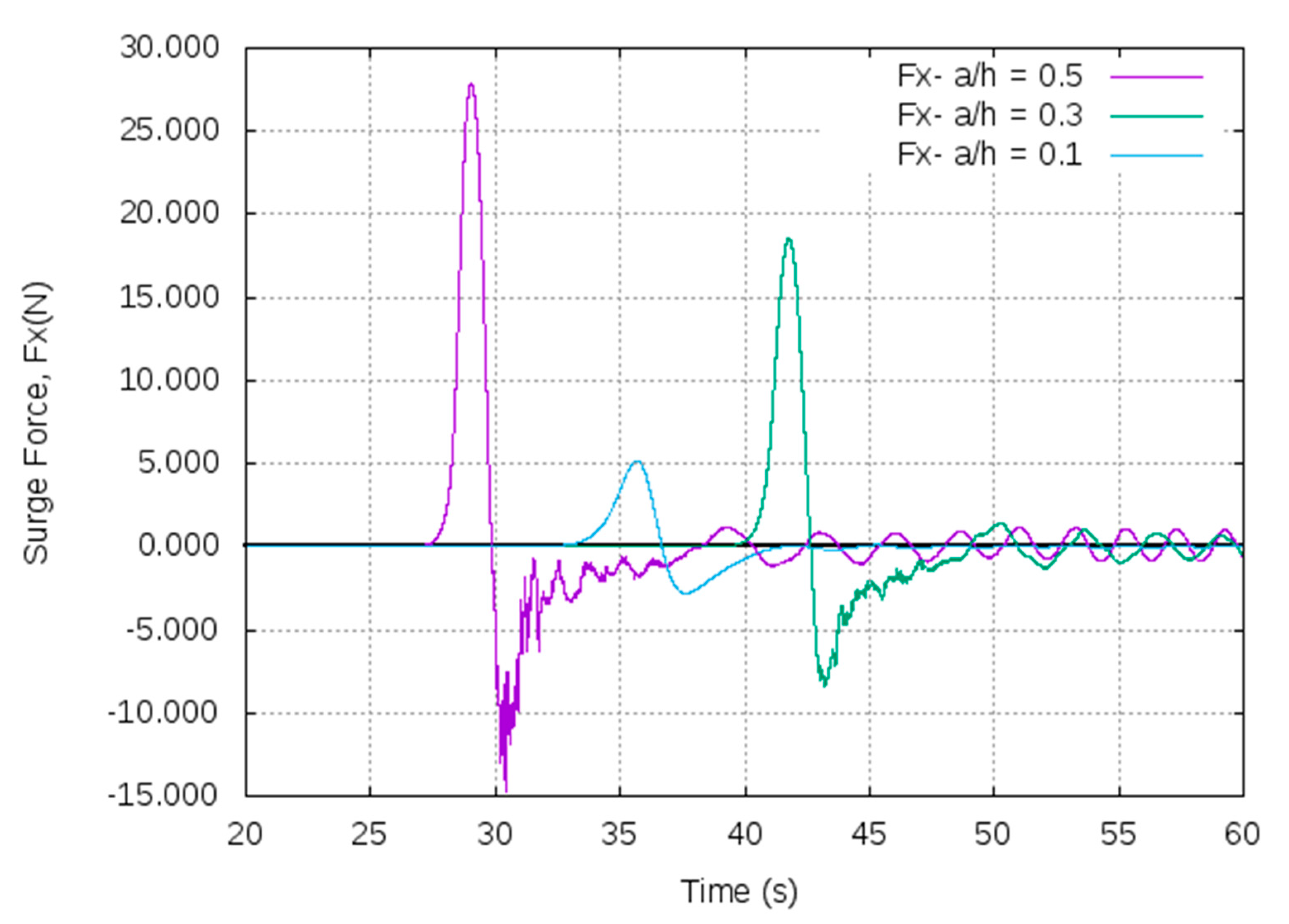
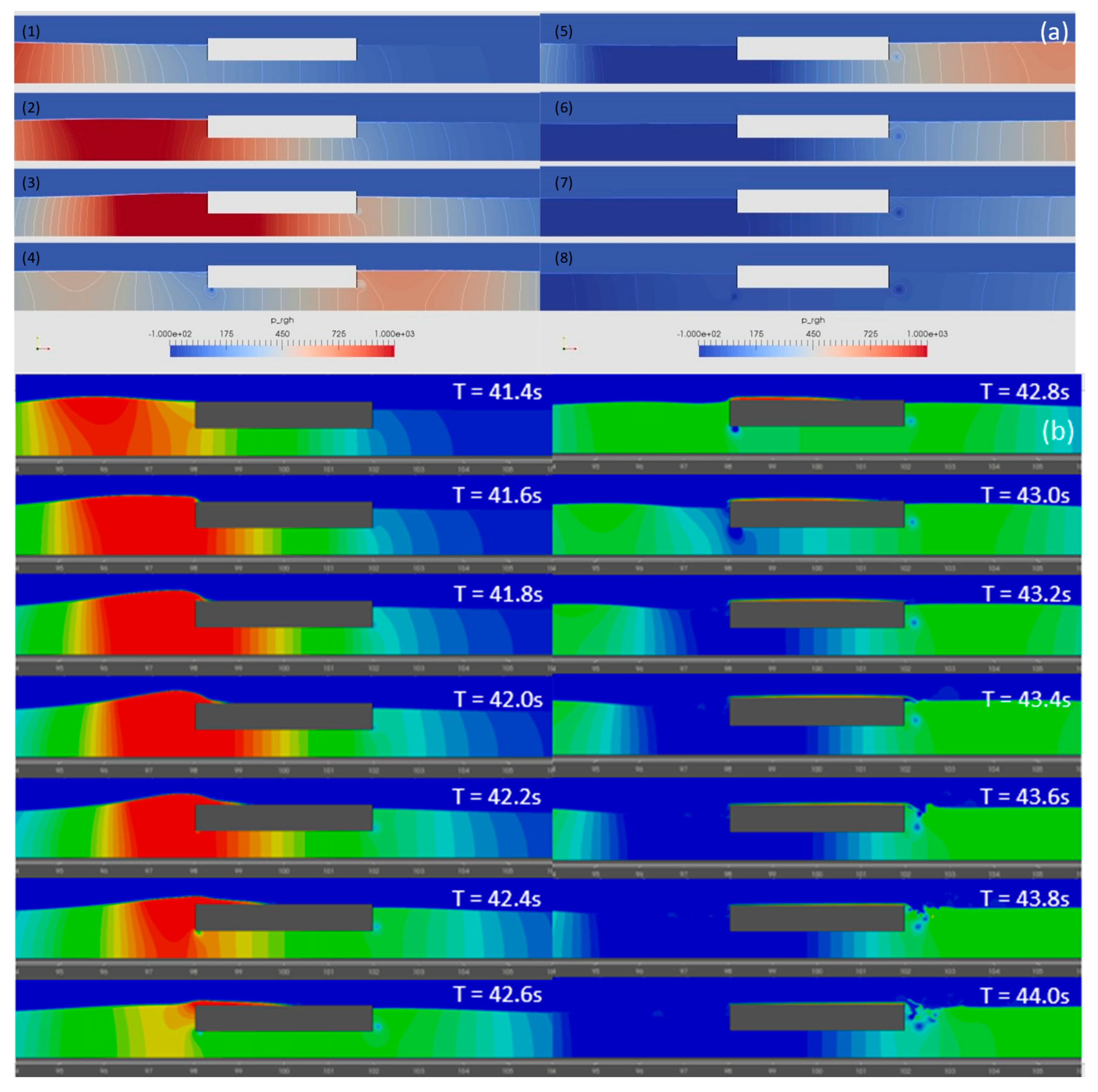
• From both the CFD and OceanWave3D, the analysis of wave forces indicated that with the increase in the amplitude of solitons, the surge and heave force gradually increase. The quantitative information is important to ensure station keeping of such structures. Further, the heave force encountered by the pontoon is substantially larger than the encountered surge force, which confirms the higher potential for application of the OWC type devices. The pressure distribution around the pontoon indicates that vortices are observed at the sharp ends of the pontoon, which might induce vibration and erosion of structure.
• The higher the initial soliton amplitude, the higher the loss of energy during interaction with the pontoon, and the higher the dissipation of energy into the dispersive tail.
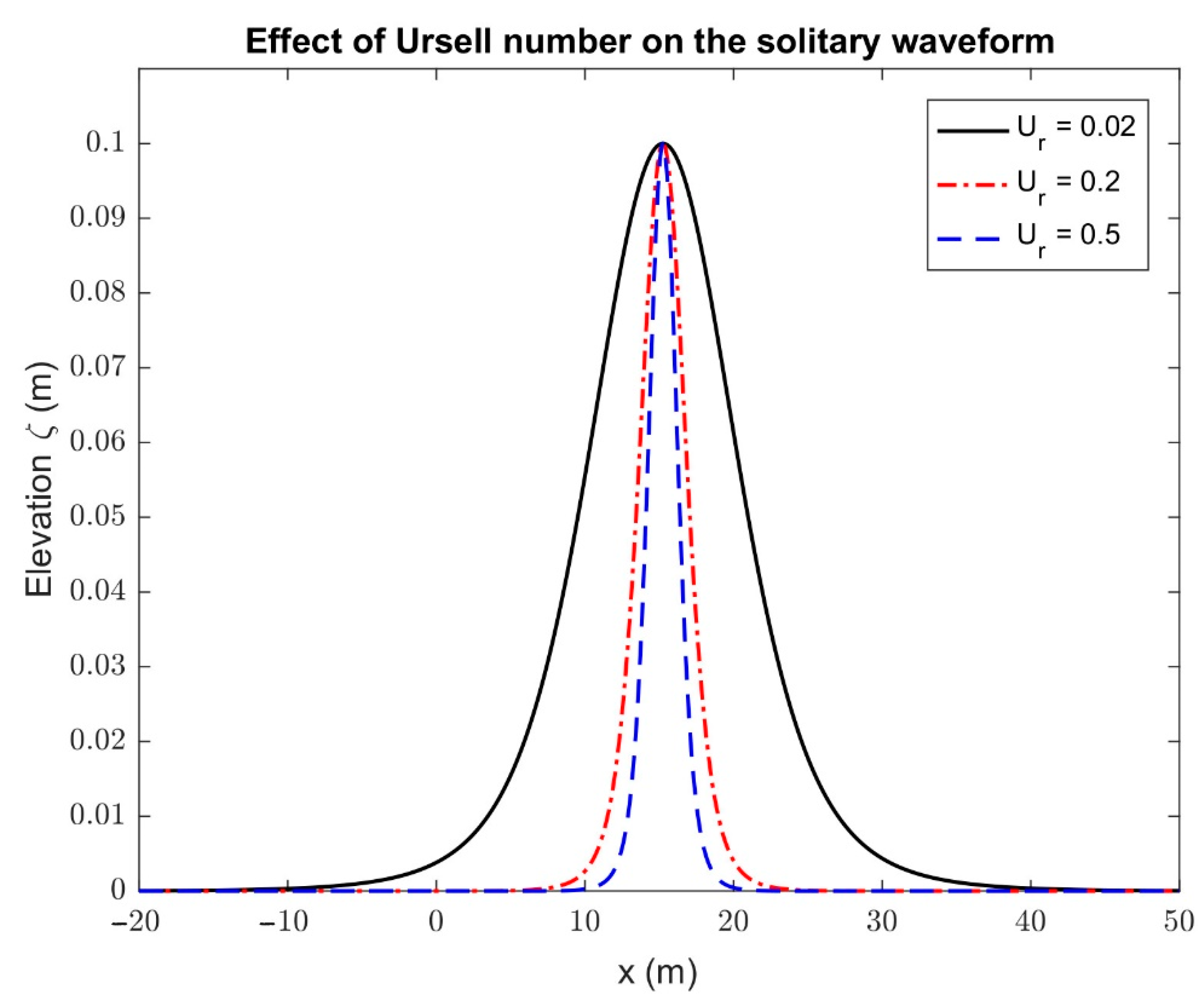
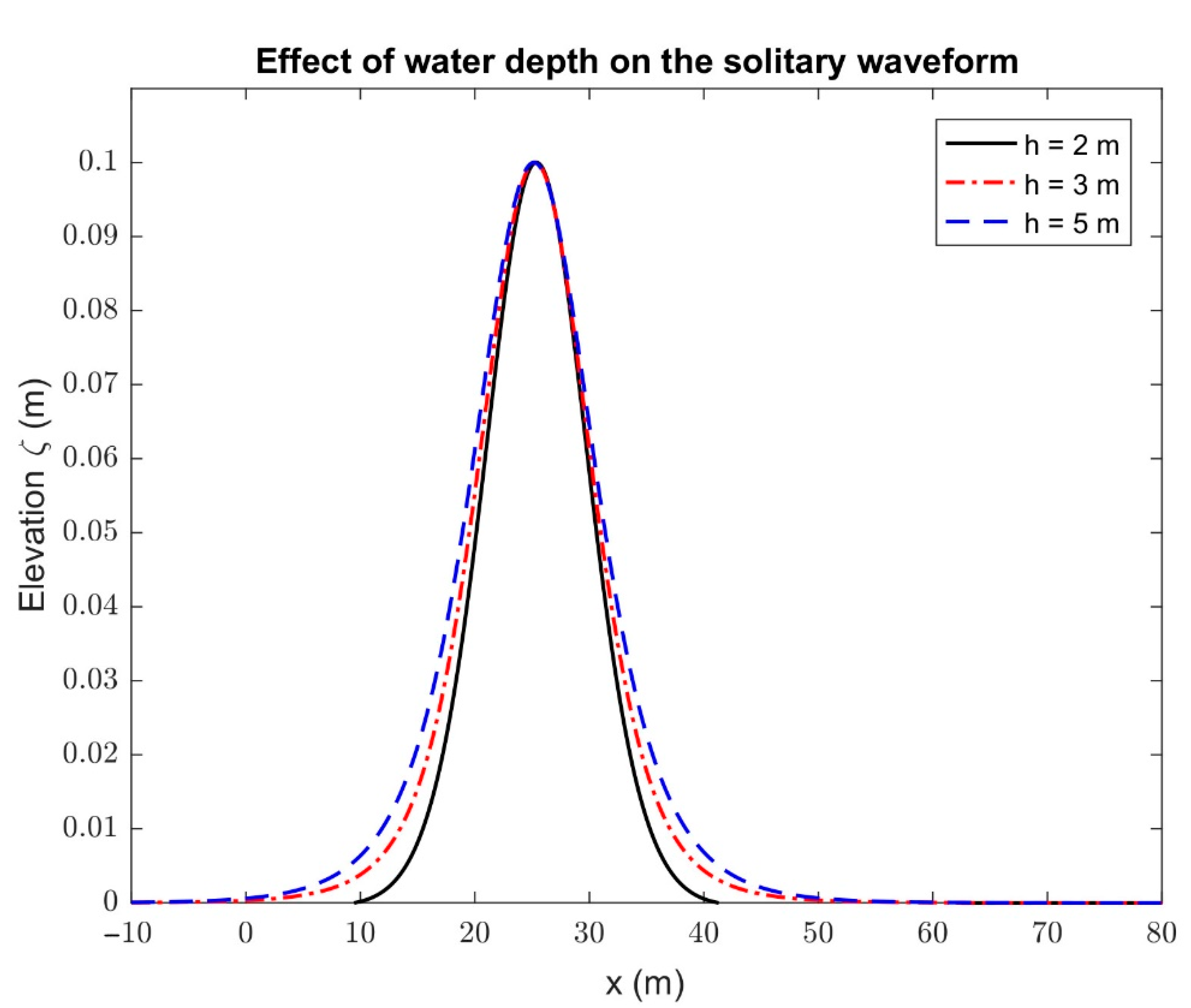
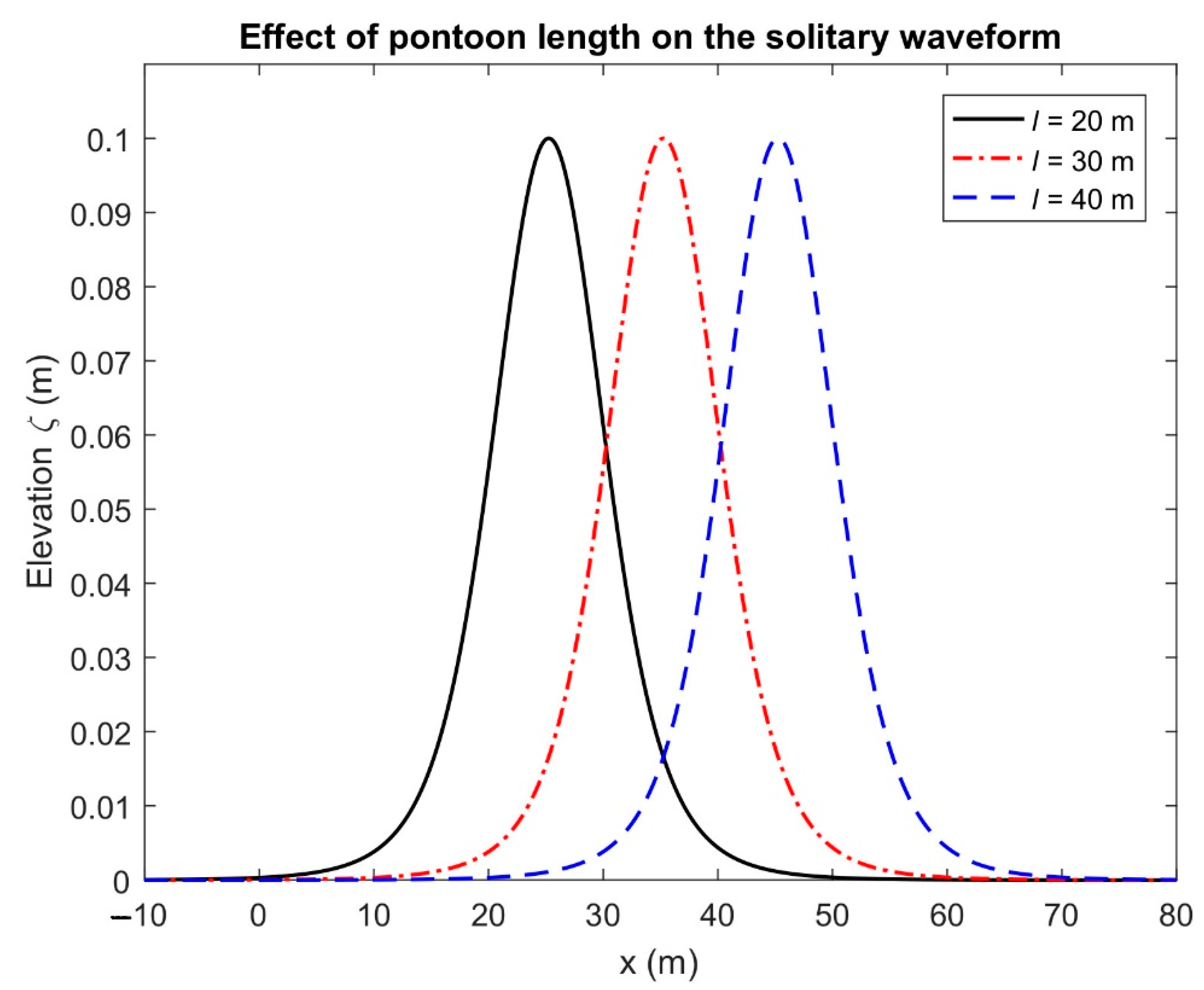
• The Ursell number has a significant effect on the solitary wave profiles than those of water depth and pontoon length.

Finally, in terms of fidelity, the RANS solution with the 2nd-order solitary wave model (OpenFOAM) shows the greatest accuracy, followed by the coupled FNPF (OceanWave3D) model. Finally, the Boussinesq formulation-based analytical solution shows good accuracy in capturing the propagating solitary wave. In terms of computational burden, the OpenFOAM model is the most expensive, followed by the coupled model (OceanWave3D), and finally the analytical model. Thus, analytical solutions may be a reliable way of obtaining initial predictions for solitary wave propagation in coastal areas, whereas coupled models may be more suitable for the study of wave–structure interaction with reliable accuracy. Therefore, the present analytical formulation will be helpful to generalize the problem of solitary wave interaction with flexible floating structure over the Boussinesq approach and comparison with different model simulations. Furthermore, future studies will attempt to expand the methodology presented herein to other types of flexible structures connected with mooring lines and it is important to investigate the hydroelastic analysis including the structural properties (flexibility and compressive force) as well as the uplift wave loads, which will not be subjected to the aforementioned limitations.

References

1. Mohapatra, S.C.; Guedes Soares, C. Comparing solutions of the coupled Boussinesq equations in shallow water. In Maritime Technology and Engineering; Guedes Soares, C., Santos, T.A., Eds.; Taylor & Francis Group: London, UK, 2015; pp. 947–954. ISBN 978-1-138-02727-5. [Google Scholar]
2. Mohapatra, S.C.; Fonseca, R.B.; Guedes Soares, C. A comparison between analytical and numerical simulations of solutions of the coupled Boussinesq equations. In Maritime Technology and Engineering; Guedes Soares, C., Santos, T.A., Eds.; Taylor & Francis Group: London, UK, 2016; pp. 1175–1180. ISBN 978-1-138-03000-8. [Google Scholar]
3. Mohapatra, S.C.; Fonseca, R.B.; Guedes Soares, C. Comparison of analytical and numerical simulations of long nonlinear internal waves in shallow water. J. Coast. Res. 2018, 34, 928–938. [Google Scholar] [CrossRef]
4. Hallak, T.S.; Islam, H.; Mohapatra, S.C.; Guedes Soares, C. Comparing numerical and analytical solutions of solitary water waves over finite and variable depth. In Proceedings of the International Conference on Offshore Mechanics and Arctic Engineering, Cancún, Mexico, 5–6 April 2021; ASME: New York, NY, USA, 2021. Paper No: OMAE2021-62642, V006T06A062. [Google Scholar]
5. Chang, C.H. Interaction of a Solitary Wave with Vertical Fully/Partially Submerged Circular Cylinders with/without a Hollow Zone. J. Mar. Sci. Eng. 2020, 8, 1022. [Google Scholar] [CrossRef]
6. Wang, Q.; Fang, Y.; Liu, H. An experimental study of run-up and loads on a vertical truncated cylinder in a solitary wave. Ocean Eng. 2021, 219, 108346. [Google Scholar] [CrossRef]
7. Mohapatra, S.C.; Islam, H.; Guedes Soares, C. Boussinesq Model and CFD Simulations of Non-Linear Wave Diffraction by a Floating Vertical Cylinder. J. Mar. Sci. Eng. 2020, 8, 575. [Google Scholar] [CrossRef]
8. Mohapatra, S.C.; Islam, H.; Guedes Soares, C. Wave diffraction by a floating fixed truncated vertical cylinder based on Boussinesq equations. In Advances in Renewable Energies Offshore; Guedes Soares, C., Ed.; Taylor & Francis Group: London, UK, 2019; pp. 281–289. ISBN 978-1-138-58535-5. [Google Scholar]
9. Lu, X.; Wang, K.H. Modeling a solitary wave interaction with a fixed floating body using an integrated analytical–numerical approach. Ocean Eng. 2015, 109, 691–704. [Google Scholar] [CrossRef]
10. Sun, J.I.; Wang, C.Z.; Wu, G.X.; Khoo, B.C. Fully nonlinear simulations of interactions between solitary waves and structures based on the finite element method. Ocean Eng. 2015, 108, 202–215. [Google Scholar] [CrossRef]
11. Xiang, T.; Istrati, D.; Yim, S.C.; Buckle, I.G.; Lomonaco, P. Tsunami Loads on a Representative Coastal Bridge Deck: Experimental Study and Validation of Design Equations. J. Waterw. Port Coast. Ocean Eng. 2020, 146, 04020022. [Google Scholar] [CrossRef]
12. Hasanpour, A.; Istrati, D. Extreme Storm Wave Impact on Elevated Coastal Buildings. In Proceedings of the 3rd International Conference on Natural Hazards & Infrastructure (ICONHIC2022), Athens, Greece, 5–7 July 2022. [Google Scholar]
13. Zhu, H.; Wang, L.L.; Avital, E.J.; Tang, H.W.; Williams, J.J.R. Numerical Simulation of Shoaling Broad-Crested Internal Solitary Waves. J. Hydraul. Eng. 2017, 143, 04017006. [Google Scholar] [CrossRef]
14. Seiffert, B.; Hayatdavoodi, M.; Ertekin, R.C. Experiments and computations of solitary-wave forces on a coastal-bridge deck. Part I: Flat plate. Coast. Eng. 2014, 88, 194–209. [Google Scholar] [CrossRef]
15. Hayatdavoodi, M.; Seiffert, B.; Ertekin, R.C. Experiments and computations of solitary-wave forces on a coastal-bridge deck. Part II: Deck with girders. Coast. Eng. 2014, 88, 210–228. [Google Scholar] [CrossRef]
16. Cuomo, G.; Shimosako, K.I.; Takahashi, S. Wave-in-deck loads on coastal bridges and the role of air. Coast. Eng. 2009, 56, 793–809. [Google Scholar] [CrossRef]
17. Istrati, D.; Buckle, I.G.; Lomonaco, P.; Yim, S.; Itani, A. Tsunami induced forces in bridges: Large-scale experiment and the role of air-entrapment. Coast. Eng. Proc. 2017, 35, 1–14. [Google Scholar] [CrossRef]
18. Martinelli, L.; Lamberti, A.; Gaeta, M.G.; Tirindelli, M.; Alderson, J.; Schimmels, S. Wave loads on exposed jetties: Description of large scale experiments and preliminary results. Coast. Eng. Proc. 2011, 32, 1–13. [Google Scholar] [CrossRef]
19. Wu, N.-J.; Tsay, T.-K.; Chen, Y.-Y. Generation of stable solitary waves by a piston-type wave maker. Wave Motion 2014, 51, 240–255. [Google Scholar] [CrossRef]
20. Goring, D.G. Tsunamis—The Propagation of Long Waves onto a Shelf. In W. M. Keck Laboratory of Hydraulics and Water Resources; California Institute of Technology: Pasadena, CA, USA, 1978. [Google Scholar]
21. Wu, N.J.; Hsiao, S.C.; Chen, H.H.; Yang, R.Y. The study on solitary waves generated by a piston-type wave maker. Ocean Eng. 2016, 117, 114–129. [Google Scholar] [CrossRef]
22. Wang, Y.; Yin, Z.; Liu, Y. Numerical study of solitary wave interaction with a vegetated platform. Ocean Eng. 2019, 192, 106561. [Google Scholar] [CrossRef]
23. Martins, K.; Bonneton, P.; Michallet, H. Dispersive characteristics of nonlinear waves propagating and breaking over a mildly sloping laboratory beach. Coast. Eng. 2021, 167, 103917. [Google Scholar] [CrossRef]
24. Gadelho, J.F.M.; Mohapatra, S.C.; Guedes Soares, C. CFD analysis of a fixed floating box-type structure under regular waves. In Development in Maritime Transportation and Harvesting of Sea Resources; Guedes Soares, C., Teixeira, Â.P., Eds.; Taylor & Francis Group: London, UK, 2017; pp. 513–520. [Google Scholar]
25. Jasak, H. OpenFOAM: Open source CFD in research and industry. Int. J. Nav. Archit. Ocean Eng. 2009, 1, 89–94. [Google Scholar]
26. Jacobsen, N.G.; Fuhrman, D.R.; Fredsoe, J. A wave generation toolbox for the open-source CFD library: OpenFOAM. Int. J. Numer. Methods Fluids 2011, 70, 1073–1088. [Google Scholar] [CrossRef]
27. Chappelear, J.E. Shallow-water waves. J. Geophys. Res. 1962, 67, 4693–4704. [Google Scholar] [CrossRef]
28. Islam, H.; Mohapatra, S.C.; Gadelho, J.; Guedes Soares, C. OpenFOAM analysis of the wave radiation by a box-type floating structure. Ocean Eng. 2019, 193, 106532. [Google Scholar] [CrossRef]
29. Engsig-Karup, A.P.; Bingham, H.B.; Lindberg, O. An efficient flexible-order model for 3D nonlinear water waves. J. Comput. Phys. 2009, 228, 2100–2118. [Google Scholar] [CrossRef]
30. Dutykh, D.; Clamond, D. Efficient computation of steady solitary gravity waves. Wave Motion 2014, 51, 86–99. [Google Scholar] [CrossRef]
31. Lin, P. A multiple-layer σ-coordinate model for simulation of wave–structure interaction. Comput. Fluids 2006, 35, 147–167. [Google Scholar] [CrossRef]
32. Rijnsdorp, D.P.; Zijlema, M. Simulating waves and their interactions with a restrained ship using a non-hydrostatic wave-flow model. Coast. Eng. 2016, 114, 119–136. [Google Scholar] [CrossRef]
33. Sarfaraz, M.; Pak, A. SPH numerical simulation of tsunami wave forces impinged on bridge superstructures. Coast. Eng. 2017, 121, 145–157. [Google Scholar] [CrossRef]
34. Istrati, D.; Buckle, I.; Lomonaco, P.; Yim, S. Deciphering the tsunami wave impact and associated connection forces in open-girder coastal bridges. J. Mar. Sci. Eng. 2018, 6, 148. [Google Scholar] [CrossRef] [Green Version]
Figure 1. Schematic diagram: solitary wave interaction with a floating pontoon.
Jmse 10 01251 g001
Figure 2. Schematic diagram of the case setup of the solitary wave scattering by a pontoon (not to scale).
Jmse 10 01251 g002
Figure 3. General mesh assembly for the study of solitary wave scattering by a pontoon—OpenFOAM mode.
Jmse 10 01251 g003
Figure 4. General mesh assembly for solitary wave scattering by a pontoon-coupled model with OW3D run.
Jmse 10 01251 g004
Figure 5. Comparisons of the solitary waveform in the outer region against CFD model simulations for different nonlinear quantities with (a) Comparison for ε = 0.1 , (b) Comparison for ε = 0.3 , (c) Comparison for ε = 0.5 , and (d) Comparison: analytical, CFD, and external numerical model [31] (see [31]) versus time t (s).
Jmse 10 01251 g005aJmse 10 01251 g005b
Figure 6. Comparison of the solitary waveform between analytical and OceanWave3D model simulations with (a) Comparison for ε = 0.1 , (b) Comparison for ε = 0.3 , (c) Comparison for ε = 0.5 versus time t (s) and (d) comparison between analytical, CFD and external numerical model [31].
Jmse 10 01251 g006aJmse 10 01251 g006b
Figure 7. Free surface elevations measured by different wave gauges along the simulation domain (see [27], a / h = 0.1 ).
Jmse 10 01251 g007
Figure 8. Relative comparison among the wave gauge results from the CFD simulations (OpenFOAM) for gauge G1 (left) and G3 (right) at a / h = 0.1 ,   0.3 ,   and   0.5 , and the results from [31] at a/h = 0.1.
Jmse 10 01251 g008
Figure 9. Surge or longitudinal force experienced by the pontoon while encountering solitary wave (for a / h = 0.1 ,   0.3 ,   and   0.5 ).
Jmse 10 01251 g009
Figure 10. Heave or vertical force experienced by the pontoon while encountering solitary waves (for a / h = 0.1 ,   0.3 ,   and   0.5 ).
Jmse 10 01251 g010
Figure 11. Pitch moment experienced by the pontoon while encountering solitary waves (for a / h = 0.1 ,   0.3 ,   and   0.5 ).
Jmse 10 01251 g011
Figure 12. Pressure distribution around the pontoon during the wave encounter in the fluid domain, while the solitary wave interacts with the fixed pontoon; (a) a / h = 0.1 , (b) a / h = 0.3 , and (c) a / h = 0.5 .
Jmse 10 01251 g012aJmse 10 01251 g012b
Figure 13. Free surface elevations measured by different wave gauges along the simulation domain a / h = 0.1 ,   0.3 ,   and   0.5 (from top to bottom, respectively; the legend is shown at the bottom) versus time t (s).
Jmse 10 01251 g013aJmse 10 01251 g013b
Figure 14. Relative comparison among the wave gauge results from the CFD simulations (coupled OF and OW3D model) for gauge G1 (left) and G3 (right) at a / h = 0.1 ,   0.3 ,   and   0.5 , and the results from [31] at a/h = 0.1.
Jmse 10 01251 g014
Figure 15. Surge or longitudinal force experienced by the pontoon while encountering solitary wave (OW3D, a / h = 0.1 ,   0.3 ,   and   0.5 ).
Jmse 10 01251 g015
Figure 16. Heave or vertical force experienced by the pontoon while encountering solitary wave (OW3D, a / h = 0.1 ,   0.3 ,   and   0.5 ).
Jmse 10 01251 g016
Figure 17. Pressure distribution (a) around the pontoon during the wave encounter (1–8 shows successive time steps) (a) OW3D, a / h = 0.1 , in the fluid domain, while the solitary wave with the fixed pontoon (b) OW3D, a / h = 0.3 , and (c) OW3D, a / h = 0.5 .
Jmse 10 01251 g017aJmse 10 01251 g017b
Figure 18. Effect of Ursell number on the solitary wave profiles in the outer region versus water plane length x (m).
Jmse 10 01251 g018
Figure 19. Effect of pontoon length on the solitary wave profiles in the outer region versus water plane length x (m).
Jmse 10 01251 g019
Figure 20. Effect of water depth on the solitary wave profiles in the outer region versus water plane length x (m).
Jmse 10 01251 g020
Figure 21. Free surface elevations measured by different wave gauges along the simulation domain for a/h = 0.3 and 0.5 versus time t (s) using OpenFOAM.
Jmse 10 01251 g021