Abstract
In this paper, we take a water quality testing Unmanned Surface Vessel (USV) as the research object. We propose a heading keeping strategy based on Human Simulated Intelligent Control (HSIC) algorithm and a trajectory tracking strategy under line-of-sight (LOS) algorithm. The practicality of the proposed control strategies was verified by combining simulations and experiments. The main contents were constructed with three parts: Firstly, we designed a complete control system of a water quality inspection unmanned boat with Arduino microcontroller as the core processor. Secondly, we derived the mathematical model of motion after reasonable simplification. Combined with the cycle experiment, the mapping relation between virtual rudder angle and motor speed was established. Then, the USV heading direction control strategy of HSIC was presented and the reliability of the proposed strategy was verified by the course control experiment of USV. Finally, aiming at the defects and shortcomings of the upper-level trajectory tracking LOS algorithm in practical application, we propose the trajectory correction and precise steering control strategies, and the practicality of the improved algorithm was verified by multi-point trajectory tracking experiments. The autonomous fixed-point water quality testing experiment was designed and verified the effectiveness of the proposed strategies.
1. Introduction
USV, a carrier for water quality testing sensors, has the ability to navigate autonomously intelligent equipment. Compared with traditional surface transport equipment, the advantages of USV are mainly to achieve unmanned control. The remote control mode of USV operation can reduce operational risk. Intelligent surface unmanned vessels have gradually become an important auxiliary tool for marine mapping, inland water transportation, water quality testing and other areas of operation. However, there are many shortcomings for USV research work. To begin, general USVs are expensive, large in size, and inconvenient to carry out experiments. In addition, the autonomous navigation control strategy needs to be combined with intelligent control algorithms to make the trajectory tracking control process more accurate and task execution more efficient in order to realize the autonomous navigation capability with lower labor cost and better control effect [,,,].
Traditional water sampling testing samples were obtained by manual operation before doing analysis. This work can also be completed efficiently by various water quality testing unmanned ship platforms and mobile unmanned ship platforms [,]. The detection method can be divided into offline detection and online detection. The representative research work of the two was proposed by Bonastre [] and Greenwood [], respectively. Scholin [] proposed a fixed underwater testing device called environmental sample processor in 2009, which regularly tested the water quality and sent the results to researchers through remote wireless transmission.
In the early 21st century, the US Naval Research Institute developed USVs including ‘Owl MK’ and ‘UHSV’. Both of them adopted sliding appearance and water jet propulsion. Through the optimization and improvement of the contralateral contour, the concealment and other capabilities were improved. In addition to military, USV also plays an increasingly important role in the civil field. Matos [] et al. took the ‘zarco’ small twin USV as the research object, and studied its dynamic positioning according to its own characteristics and external interference. Breivik [] et al. developed the ‘kaasball’ USV and tested its mobility and agility. A team from China naval engineering university completed the actual lake test experiment using the developed ‘sturgeon 03’ USV [].
For the motion control of USV, the realization of its function is completed by the bottom layer of heading control and the upper layer of trajectory control, which is the essential problem of convergence control of heading angle and position error [,,,].
The research on heading control of USV is closely related to the development of an automatic rudder, and its performance directly determines the effectiveness of the realization of heading keeping, heading change, and trajectory tracking. Wu [] et al. proposed a heading tracking strategy for vessels with unknown time-varying parameters, completely unknown time-varying control coefficients, and unknown time-varying bounded environmental disturbances. Fang [] et al. proposed a new adaptive heading controller based on backpropagation neural network and artificial bee colony algorithm, and the simulation results showed that the system parameter error control under this method was within the acceptable range. A robust localization algorithm was proposed by W Choi [] for a USV using Double Deep Q-Network with Action Memory. Y Qi [] et al. studied observer-based model predictive control. Mmi [] et al. proposed a robust integral backstepping and terminal cooperative controller to achieve good heading keeping performance, and reduced the energy consumption during the USV heading keeping control. The path tracking control problem of USV with unmodeled dynamics, external disturbances, and input saturation was studied by B Qiu [] et al.
The USV trajectory tracking process is to plan the desired track to be tracked in advance. According to the different requirements of the actual work scenarios, the designed intelligent tracking control algorithm is combined to control the USV trajectory on the desired route and continue to sail along the trajectory.
The LOS control algorithm is widely used in practical tracking control because of its simple structure, no complex integration, and iterative computation in the control process. In spite of this, the method well meets the real-time requirements, while not being limited to the situation where the parameters of the controlled object model are difficult to determine. Maurya [] et al. designed an inner and outer loop control structure, which was characterized by the decoupling of the inner and outer loops and the fact that the design of the outer loop controller does not need to consider the dynamics model of the designed object. Min B [] et al. proposed a robust track keeping control strategy for vessels with indirect nonlinear feedback in order to solve the problem that the parametric line-of-sight guidance algorithm cannot be directly applied to practical navigation. Gonzalez-Garcia [] et al. combined deep neural network with the LOS algorithm to design an adaptive controller, and simulation results showed that the controller was able to self-learn to achieve the desired speed and yaw dynamics regulation. Lee [] et al. designed an autonomous navigation strategy for jellyfish removers based on the LOS algorithm, and applied it to practical removal work.
Based on the above research, we independently designed an intelligent water quality monitoring unmanned boat that can control the course and track the trajectory. In Section 2 we elaborate the control system of the water quality monitoring unmanned vessel, describing in detail the modules of the upper and lower computer and the functions. In Section 3 we derive the mathematical model of the unmanned ship by reasonable simplification. Section 4 and Section 5 are the main contributions of this paper; we describe the HSIC-based heading control strategy and the LOS-based trajectory tracking strategy, which are the main elements of the control system design in this paper. Immediately afterwards, we conducted several experiments to verify the effectiveness of the above two algorithms. Thereafter, the unmanned vessel was finally used successfully in water quality testing experiments.
2. Water Quality Testing Unmanned Surface Vessel Control System
2.1. Design Selection
We used the double propeller drive whose maneuverability and flexibility of operation can be well-controlled accurately as the drive device of the USV. As shown in Figure 1 this paper designs and manufactures the assembled small water quality testing Unmanned Surface Vessel experimental prototype.
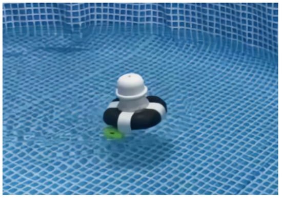
Figure 1.
Physical diagram of the USV.
Then the main parameters of the USV are shown in Table 1.

Table 1.
Main parameters of the USV.
2.2. Lower Computer Control Platform
The lower computer control platform mainly involves the software and hardware equipment of the USV. The propulsion device of the USV is composed of two brushless DC motors. The rotation of the motor is controlled by the pulse width conditioning signal provided by the microcontroller.
The control system of the USV includes two parts: the hardware part takes the microcontroller as the center and is externally connected with the sensor components of environmental sensing (positioning sensor and inertial measurement sensor) and water quality signal acquisition. The software part consists of data analysis, heading control, trajectory tracking algorithm, and so on.
Table 2 shows the hardware list of the USV control system, including micro control unit, dynamic sensing unit, wireless network communication unit, and water quality detection unit.
Table 2.
Hardware list of control system.
The total number of digital I/O pins of Arduino mega2560 micro control unit is 54 pins, including 15 PWM pins, 16 analog input pins, and 4 UART serial ports; it is the motherboard and contains the main control unit. In the dynamic sensing unit, the GPS positioning module adopts NMEA0183 protocol, which can extract effective information such as longitude, dimension, and ground speed through code analysis so as to obtain the real-time position information of the USV. The inertial measurement unit JY901 can accurately output the real-time attitude angle, angular velocity, and other information of the USV through the solver and filtering algorithm. By using the GPRS unit, remote wireless network communication can be realized, and control command distribution and data upload can be completed. The SIM card is mainly used to store the identification data of the unmanned ship. By communicating with nearby base stations, it ensures both the mobility of the unmanned ship and the ability to quickly locate the new position of the unmanned ship after it moves. In spite of this, the SIM card can also store temporary commands and data issued by the upper computer. Based on the USV platform, by carrying three kinds of water quality detection sensors (temperature sensor, turbidity sensor, and pH sensor), the pollution degree of the water area to be tested can be roughly mastered. In the driving unit, the motor controller is an integrated circuit that controls the motor to work according to the set direction, speed, angle, and response time by working actively. The motor driver is used in pairs with two motors, and the speed adjustment of the motor is realized through the control signal output by the micro control unit.
The hardware diagram of the unmanned ship control system in this study is shown in Figure 2, which shows the composition and function of each functional unit of the control system.
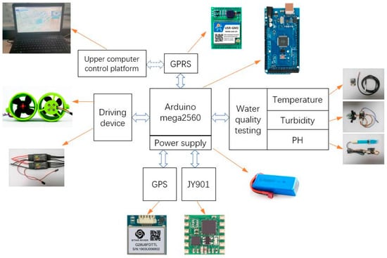
Figure 2.
The upper computer presentation layer interface.
2.3. Upper Computer Control Platform
2.3.1. Control Platform Functions
The upper computer server was built in China, and the link of the website is http://www.cheerstech.cn/system/ (accessed on 4 August 2022). By accessing Baidu map API (https://api.map.baidu.com/lbsapi/cloud/index.htm accessed on 4 August 2022), the position display and trajectory point setting of USV can be realized.
Figure 3 shows the upper computer interface, which includes user device management module, data display module, network remote control module, and trajectory tracking point selection module. The main function of the network remote control module is to realize the backward and forward sailing movements of the USV so as to facilitate the recovery of the USV and other work.
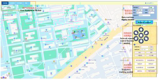
Figure 3.
The upper computer interfaces.
The trajectory tracking point selection module mainly selects a series of target points in the actual open water through Baidu map interface, and the front and back points are connected into line segments in turn to form the desired track, and sends the information to the microcontroller through GPRS for temporary storage pending further processing.
2.3.2. Parameter Configuration
Before the remote network communication, the upper computer needs to be configured with relevant parameters. The initial configuration options on the server side of the upper computer include parameters such as IP address, port number, connection type, baud rate, device ID, etc. The detailed configuration information is shown in Table 3.
Table 3.
Server configuration parameters.
When the water quality testing Unmanned Surface Vessel is in motion control, its position, attitude, and other details need to be sent to the upper computer for display and record keeping in accordance with the custom field format in order to detect the motion status of the USV and water quality testing in real time. In the built-in code of microcontroller, the data are continuously sent through GPRS cycle according to the set format.
3. Mathematical Model of Unmanned Surface Vessel
3.1. Mathematical Model of Motion
For the spatial motion state of the USV, the geodetic coordinate system and the hull coordinate system can be combined to describe the spatial motion state of the USV. In Figure 4a, the geodesic coordinate system is commonly used to describe the position and attitude of an unmanned ship. The hull coordinate system was adopted to describe the relative motion of the unmanned ship to the water body.
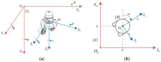
Figure 4.
(a) Space motion coordinate system; (b) simplified coordinate system for plane motion.
In the coordinate system , and are defined as the position vector and attitude vector of the unmanned ship, where x, y, and z denote transverse, longitudinal, and vertical displacements, respectively. Moreover, , and denote the heel angle, trim angle, and heading angle, respectively. Thus, the generalized displacement of the unmanned ship in the coordinate system can be expressed as .
In the coordinate system , and represent the linear and angular velocity vectors of the unmanned ship, respectively. According to the definition, u, v, and w denote forward, traverse, and droop speeds, respectively. Moreover, p, q, and r denote the horizontal, vertical, and bow angular speeds, respectively. Thus, the generalized velocity of the unmanned ship in the coordinate system can be expressed as . In the actual motion, the motion in six degrees of freedom in space can be reduced to the motion in three degrees of freedom in the horizontal plane because the motion in the drape, transverse, and longitudinal rocking directions has less influence on the unmanned ship. Under this circumstance, and . Figure 4b shows the top view of the simplified motion coordinate system of the unmanned ship in the horizontal plane.
Considering that the appearance of the USV designed in this paper is a circular ring structure, which can be approximately regarded as a completely symmetrical structure, it can simplify the motion mathematical model to a great extent, reduce the difficulty of modeling, and lay a foundation for subsequent research.
To simplify the analysis, the following four assumptions are considered to obtain the horizontal plane mathematical model of USV.
- The hull is symmetrical from left to right and from front to back, ;
- The coordinate origin of the hull coordinate system coincides with the center of gravity with ;
- Considering only the motion of the horizontal plane of the vessel load and ignoring the effect of transverse, longitudinal, and bow rocking motion, we set ;
- The influence of model uncertainty and external disturbance can be ignored.
It can be obtained as follows:
where denotes the transformation matrix, is a symmetric positive definite matrix, for a rigid body moving in a fluid the centripetal force matrix has skew-symmetric properties, the damping matrix is asymmetric and positive definite, denotes the system control input, and and are the longitudinal force and steering moment, respectively.
According to the vessel motion knowledge, when the shape of the USV is symmetrical, the change in the longitudinal motion speed of the USV does not cause the transverse force and rotation torque, and is obtained. The change in caused by the change in and is symmetrically distributed, that is is the even function of and , which satisfies . Similarly, when the USV is symmetrical, and are satisfied.
Then we perform the following analysis. represents the hydrodynamic change in X direction caused by changing the longitudinal velocity u by a unit value when and are established. represents the hydrodynamic change in Y direction caused by changing the transverse velocity v by a unit value when and are established. Combined with the circular ring structure of USV designed in this paper, it can be seen that is equivalent to , and their derivatives are consistent, with .
The final collation leads to the mathematical model of the motion of USV on the horizontal plane as:
where , , . x, y, z denote transverse, longitudinal, and vertical displacements, respectively.
3.2. Mathematical Model of Propulsion
Unlike traditional surface vessels that rely on steering by steering rudder, the propulsion power source of the USV designed in this paper is provided by two symmetrically installed propeller thrusters at its stern, and the steering is controlled by the speed difference between the two motors, so it is necessary to analyze these two speed parameters and the thrust and torque they generate, and establish a mathematical model between them, as well as to facilitate subsequent research.
The schematic diagram of a USV under the propulsion of two propeller thrusters is shown in Figure 5. In practice, the two propellers generate two parallel thrusts and , respectively, and adjust the rotational speed to generate the driving force and steering torque . Thus, the calculation formula of thrust of single propeller is []:
where is the water density; and denote the speed magnitude of the left and right propulsion motors of the USV, respectively; is the propeller diameter; is the thrust coefficient. The torque can be calculated as:
where denotes the torque coefficient. For the motion control of the USV designed in this paper, the control objects are thrust magnitude and rudder angle, both of which can be related to the rotational speed of the left and right propulsion motors installed at the stern of the USV, the speed of navigation is positively related to the rotational speed of the motors, and the steering is equally positively related to the difference in rotational speed of the motors. The equation of the relation vessel between the virtual rudder angle and the left and right motor rotational speed is:

Figure 5.
Schematic diagram of USV propulsion system.
In the above equation, the value of the proportionality coefficient can be determined by simulation and actual experiment; is the artificially set rudder angle adjustment boundary value, take . The above equation involves two motor speeds, for the purpose of algorithm design and implementation a reference speed is defined, the control amount in the control system is reduced to control alone, and the left and right motor speeds can be described as:
Thus, can be further calculated as:
where represents the adjustment speed of the left and right motors increased or decreased on the basis of the base speed , with represents the direct motion of the USV. The purpose of designing the absolute value of the change in speed of the left and right motors is that one can reduce the control volume, and the other is that the steering is simulated when the steering is controlled, and when the absolute value of the change in speed of the two motors is the same, the steering can be ensured to be smoother.
3.3. Morporation of Virtual Rudder Angle and Speed
After establishing the mathematical model of the motion of the USV and the design and selection of the propulsion system, this subsection obtains the relevant parameters through a series of cycle experiments of the USV on this basis, and obtains the mapping table between the virtual rudder angle and the left and right motor speed and , respectively, by combining the rudder angle simulation experiments and the actual experiments, the specific data are shown in Table 4.
Table 4.
Mapping table between virtual rudder angle and speed and .
It can be seen from Table 4 that with the change in virtual rudder angle or motor speed, the change in cycle radius and speed presents a certain linear law. After simple fitting of tabular data, the following two laws can be obtained: When the actual speed is less than or equal to 0.98 m/s, it meets the requirements , , . When the actual speed is greater than 0.98 m/s, it meets the requirements , .
4. Heading Control and Trajectory Tracking Algorithms
4.1. Heading Control Based on HSIC Algorithm
4.1.1. HSIC Algorithm Improvement
The HSIC algorithm generates a simple and practical control effect with online adjustment function by summarizing and recording certain actual human behavior, control experience, and various intuition-based logical reasoning.
The basic form of the algorithm is []:
where is the control output of the controlled system, and and denote the th and th hold values of the control system output, respectively. is the proportional control module, is the suppression factor , is the proportionality factor, and are the deviation and derivative generated by the system, respectively.
Modifying the proportional control module in the HSIC algorithm to a PID control module, the improved HSIC control algorithm is:
where can be understood as the system control output increment after PID control module discretization through the processing of this design method to avoid the defects of traditional PID deviation accumulation. When the control state occurs abnormal changes can output normal values, . indicates the inhibition or gain coefficient, whose value is determined by the actual navigation state.
4.1.2. Control Level Design
Combined with the actual navigation control mode of the designed USV, the dynamic characteristics of HSIC are divided into multiple regions in the error phase plane, while regions with the same properties are grouped together to establish five dynamic characteristics control modes, as shown in Figure 6.
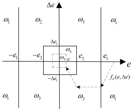
Figure 6.
Phase plane diagram of HSIC.
The dashed line with arrows in the figure indicates the target track with ideal deviation of the track for the five characteristic patterns in the figure. According to the actual navigation situation the following analysis can be performed.
- Feature mode : . Which reflects that the actual heading angle of the USV deviates greatly from the target heading. The difference in the sign of deviation e between quadrant one and four and quadrant two and three in the figure reflects the left or right deviation in the actual heading. At this time, in order to track the target heading as soon as possible, it is necessary to execute the maximum position of the rudder command (control the maximum speed difference between the left and right motors) in order to control the USV to perform a larger steering action;
- Feature mode : . The deviation and are both in a wide range. makes have a decreasing trend, and the PID control module is multiplied by the suppression factor to ensure the and the to decrease further;
- Feature mode : . Both and are in a large state, and the makes the change in the direction of increasing. A stronger PID regulation control is needed to achieve rapid convergence of deviation, so the gain factor is multiplied by the output of the original PID control module;
- Feature mode : , . and are small, and the PID control module is used to update the system output by continuously calculating the increment of the deviation;
- Feature mode : , ( is a very small positive number). and are very small, and at this time can be considered to have completed the tracking, the system control output remains unchanged. The output of the next moment and the current output value is the same, reflected in the motor by the consistent interval moment motor speed, maintaining the current heading state.
Based on the above five eigenmodes, combined with the improved HSIC control algorithm, the set of eigenmodes is given as .
The control model set corresponding to the above five characteristic modes is defined as . The five control modes formed within the modal set are designed as:
where and are the control outputs (i.e., left and right motor speeds) of the system at the th and th sampling moments, respectively. is the maximum steering rudder angle value (corresponding left and right motor speed values can be obtained from the rudder angle and speed mapping in Table 4), and is the control input of the system, which means the deviation of the heading angle at the th sampling moment, and reflects the change in the deviation before and after the sampling moment, which is equivalent to (which is the angular velocity of the heading measured by the attitude sensor). and are the target heading and the actual heading at the kth sampling moment, respectively.
4.1.3. Control Parameters
The excellent PID control parameters in different control states in the early stage were recorded and sorted into a control parameter table. In the control process, the HSIC control algorithm, by constantly judging the control deviation and its change trend, selects the corresponding control mode and a group of appropriate parameters for motion control in combination with the previous control parameter table.
According to the experimental data in Table 4, the relation vessel between the system output quantity (rudder angle) and the USV state condition (heading angle) can be obtained. In the actual experiment, the deviation and deviation change quantity threshold values are set as , rad/s, the inhibition coefficient is taken as , and the gain coefficient is taken as . The PID comparison simulation test was designed and the effectiveness of the improved algorithm was verified by the simulation results. Table 5 shows the table of control parameters recorded during the preliminary experiments, which lays the basic data for the control implementation of the improved algorithm.
Table 5.
The record table of control parameters.
In order to achieve better control effect and accuracy in the actual control process, it is necessary to numerically adjust the control parameters , , and in the PID control method based on the USV model. After several experiments, a better set of parameters , , and was selected to control the heading at 45°, 90°, and 135° N.E. The simulation comparison experiments were conducted under the unit step signal as the input response, and the initial heading was set at 135° N.E. The simulation results are shown in Figure 7, Figure 8 and Figure 9.
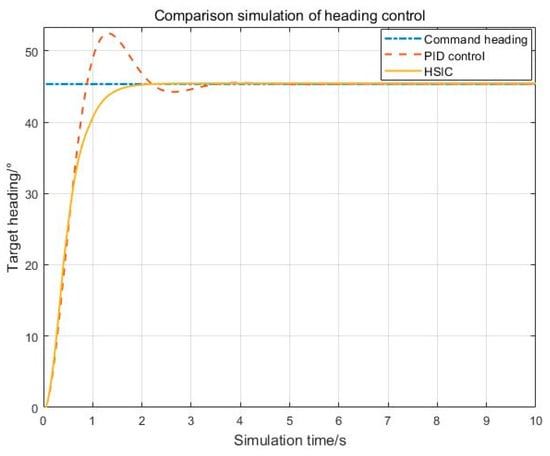
Figure 7.
The 45° heading simulation comparison chart.
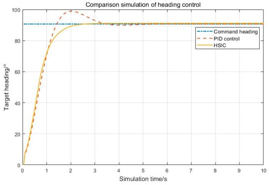
Figure 8.
The 90° heading simulation comparison chart.
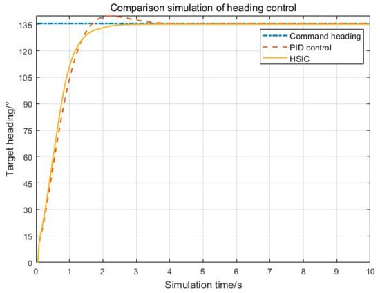
Figure 9.
The 135° heading simulation comparison chart.
From Figure 7 to Figure 9, it can be seen that the HSIC control algorithm has faster response speed, smaller overshoot, and shorter time required to track the upper target heading, while the tracking under the traditional PID control method produces a larger error and tracking effect which is not as good as the control algorithm designed in this paper. Despite this, the deviation convergence control capability of HSIC control algorithm was initially verified through the heading control comparison simulation test, which has certain significance for the bottom heading motion control of USV, and can better execute the bottom control command, and then lay the bottom foundation for the subsequent upper trajectory tracking control.
Figure 10 shows the flow chart of HSIC control algorithm execution. The algorithm execution process starts from the serial data reception and sensor data reading, which includes the measured heading angle , the target heading angle , and the measured heading angular velocity , that is, the deviation change amount , , and are the human-set deviation and deviation change amount threshold values, respectively, and the suitable threshold value was selected through the actual heading control experiment. By comparing the deviation and the deviation change with the set threshold, the USV was controlled to perform the navigation modes of left turn, right turn, and heading hold to achieve more efficient heading tracking.
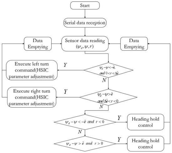
Figure 10.
HSIC algorithm flow chart (Y: Yes, N: No).
4.2. Trajectory Tracking Control Based on LOS Algorithm
The main function of the line-of-sight (LOS) guidance algorithm is to generate the desired heading angle according to the position and heading error between the actual position and the target point, and then the USV adjusts the left and right motor speed to change its heading , and continuously adjusts to make the error between it and the desired heading angle reach the allowable range []. The process of controlling the motor speed to realize the constant convergence of the heading error needs an implementation strategy. The designed HSIC control strategy is used to realize the upper-level heading tracking by means of the bottom-level control, which is combined with the upper-level trajectory tracking control strategy to finally realize its automatic control strategy for trajectory tracking in line with the actual application.
4.2.1. Track Correction
The trajectory correction diagram of USV is shown in Figure 11. When the deviation between the actual position of the USV and the track to be tracked is larger than the line-of-sight radius in the LOS algorithm, the line-of-sight point ceases to exist, thus introducing a fast deviation correction strategy to adjust the rudder angle to control the heading, and then switching to the LOS control mode when the deviation of the track is smaller than the line-of-sight radius.
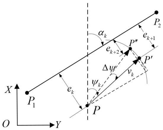
Figure 11.
Fast correction strategy.
The current heading angle of the USV in the figure is , the speed is , the sampling interval of the sensor is set to , the sampling moment is at the moment . Assume that after the next sampling interval , the position of the USV is updated to , the deviation is updated to . In order to quickly adjust its heading, if the steering rudder angle is adjusted at the moment so that the heading changes , then the position at the next sampling interval is , and the deviation is . According to the geometric relation vessel, it is known that:
When , there is . Then we would have:
It is known that:
In this equation, can be interpreted as the predicted value of the deviation of the track at the next sampling moment, which is positively correlated with the change in heading angle . Therefore, the change in heading can be predicted based on the deviation value, so that the heading can be adjusted to gradually follow the target track. The next step is to establish the relation vessel between the rudder angle and Equation (23).
From the first order linear Nomoto model, it follows that:
where and denote the slewability index and rudder index, respectively, and the special solution of Equation (24) in one sampling period is:
At the same time, it can be seen that:
It can be solved simultaneously:
Thus, the target rudder angle for control is finally derived, and the corresponding steering rudder angle value is then output using the prediction of the amount of change in the trajectory deviation at the next sampling moment to realize the correction process. In the experiment, the target rudder angle E is obtained by taking , , and the sampling interval . Combining the rudder angle and speed mapping table in Table 4, the control speed of the left and right motors can be obtained at the next moment, thus gradually reducing the deviation, and completing the correction of deviation.
4.2.2. Steering Control
The trajectory tracking process based on the LOS algorithm is generally composed of straight line segments to be tracked, and because there is a discontinuous first-order derivative at the intersection of straight line segments, it leads to a degradation of maneuvering performance when the USV passes through this steering point. Moreover, if a transition is achieved by introducing circular arcs between adjacent straight line segments, the steering maneuverability is improved []. However, this treatment results in setting the track point which does not pass through the intersection of straight line segments, and this method is inadequate when encountering close maneuvers and requiring more accurate trajectory tracking (e.g., obstacle avoidance requirements, etc.). The next step is to design a control strategy for precise steering and passing through the steering point during the steering process by studying the straight line segment and the arc connection.
Figure 12 shows the schematic diagram of steering arc connection, and Figure 12b improves the circular arc segment based on Figure 12a, so that the steering track passes through the intermediate track point, which can improve the accuracy of trajectory tracking. Suppose denotes a series of preset target points while a reasonable radius of steering arc is set, and is taken in the experiment, and the center of circle is on the angle parallels of two adjacent straight line segments. For the relative positions of the circle centers in Figure 12b, there are:
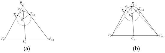
Figure 12.
Steering arc connection. (a) Before improvement. (b) After improvement.
In order to further analyze the steering tracking problem, we set four track points and control the USV to track them in turn. Meanwhile, according to the difference of the track point position, the circular arc section track can be divided into two cases of clockwise steering and counterclockwise steering. At this time, the track control problem is transformed into the solution of the tangent point of each linear segment and the rotation angle of the circular arc segment. After the tangent point and the rotation angle are determined, the precise steering control of the USV can be realized by combining the set steering radius, as shown in Figure 13 and Figure 14 for the relation vessel between clockwise steering and counterclockwise steering of the circular arc segment, respectively.
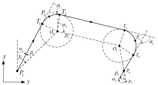
Figure 13.
Clockwise turning circular segment.
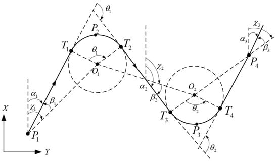
Figure 14.
Counterclockwise turning circular segment.
The cis-reverse steering relation vessel of the circular segment can be expressed as:
where denotes the rotation angle of two adjacent linear segments, denotes clockwise steering, denotes counterclockwise steering, and the rotation angle of the circular arc segment can be expressed as:
At the same time:
Thus, after solving for the tangent point and the starting point of the line and the circular arc segment, it follows that:
where , it can be expressed as:
5. Experiments and Discussions
5.1. Heading Control Experiment
This subsection combines the USV designed in this paper to conduct experiments in actual waters with set heading keeping (145° N.E.) to verify the practicality and effectiveness of HSIC control algorithm. The experiment in the actual water was carried out as follows; Firstly, two points were selected through the upper computer wireless network control platform, i.e., the starting point S and the ending point E. A straight line was automatically connected between the two points, and the upper computer platform sent the latitude and longitude information of the two points to the USV, and then the USV was remotely controlled to navigate to the waters attached to the starting position through the network remote control mode, and then entered the automatic navigation mode. The initial heading of the USV deviated from the desired heading, and as the internal microcontroller continuously makes logical judgments on the deviation and the amount of deviation change by using the collected heading angle data, the USV gradually adjusted its heading angle and its own attitude, and effectively tracked the set target heading. Its tracking process maintains the approximate linear motion within the set heading deviation of ±4°, advances continuously, and tracks to the end position E annex waters, completing the heading tracking control experiment.
Figure 15 represents the graph of the experimental data of heading control based on HSIC algorithm, in which the horizontal coordinate is longitude, the vertical coordinate is latitude, and the blue line indicates the latitude and longitude coordinates collected in real time during the course of USV heading tracking.
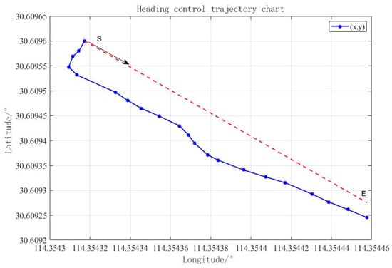
Figure 15.
The experiment of heading control based on HSIC algorithm.
Figure 16 represents the graph of heading angle change. The experimental data of heading control show that the USV sails the whole length of about 33.35m, and its heading angle error is kept within ±4° when the heading is stable. From Figure 15, it can be seen that the USV has a large deviation of heading at the beginning, and after the regulating effect of HSIC control algorithm, its heading gradually tracks on the set heading and keeps on, because there is no tracking control of the track distance in this process, so when the USV’s heading tracks on the target heading, the vertical error of its track and the line connecting the set starting point and end point cannot be eliminated; this problem is studied and solved in the next section. Figure 17 shows the actual navigation of the unmanned ship executing the command of 145° N.E. Figure 17a represents the start of the heading tracking phase. Figure 17b,c represent the two different phases of heading control, respectively.
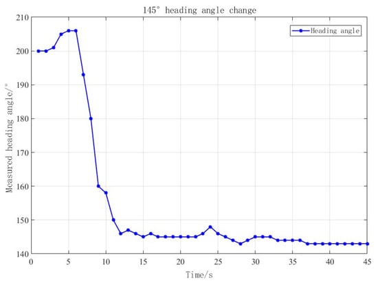
Figure 16.
Changes in heading angle.
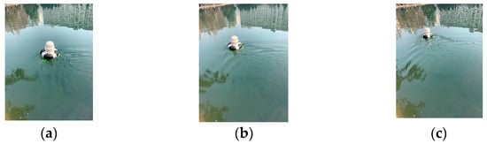
Figure 17.
The 145° N.E. heading control experiment. (a) Phase 1; (b) Phase 2; (c) Phase 3.
5.2. Multi-Point Trajectory Tracking Experiment
Combined with the improvement of the LOS algorithm control strategy in the above subsections, this section aims to design a set of LOS-based trajectory tracking algorithm control logic to facilitate the subsequent experimental validation work.
The design flow of the trajectory tracking program is shown in Figure 18, and the corresponding microcontroller control program was designed relying on this flow so as to realize the trajectory tracking experiment.
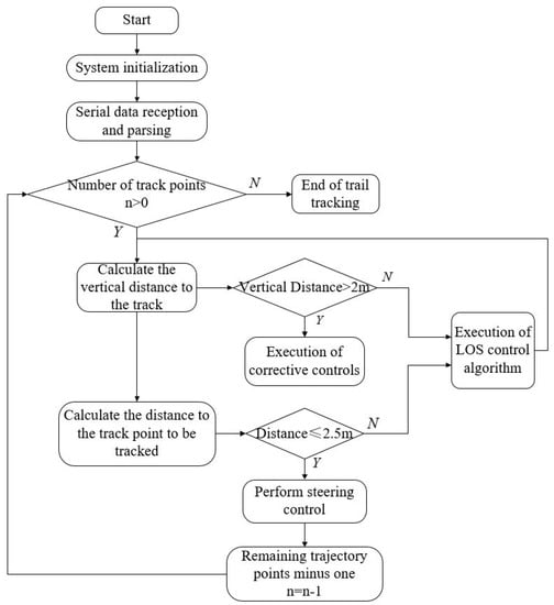
Figure 18.
Flowchart of trajectory tracking program design (Y: Yes, N: No).
To verify the practicality and effectiveness of the proposed tracking algorithm, it was compared with the traditional LOS algorithm before improvement to design the autonomous tracking experiments of USVs, and the collected experimental data were analyzed and compared.
5.2.1. Refractive Line Tracking Experiment
For the bending trajectory tracking experiment, firstly, three trajectory points were set in the remote network control platform, and the points were connected to each other to form the target trajectory to be tracked, and then the USV was controlled to sail to the first point attachment first, and then the control platform issued the autonomous tracking navigation command to control the USV to pass the second and third points in turn to complete the trajectory tracking experiment. The advantages of the improved algorithm were verified by the experimental results.
Figure 19 shows the trace tracking control before the algorithm improvement, including the position tracking graph and error analysis graph, combined with the experimental data results can be seen: the full length of 113.2 m, the maximum error reached 3.4 m, and the average tracking error is 2.24 m. Figure 20 shows the tracking experimental results after the algorithm improvement. The maximum error is 2.45 m and the average tracking error is 1.31 m after the tracking experiment by the improved algorithm. The average tracking error is 1.31 m, and the tracking effect is better.
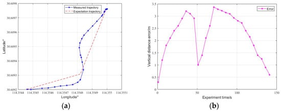
Figure 19.
Experiment of bending trajectory tracking before improvement. (a) Folded trajectory; (b) track tracking error.
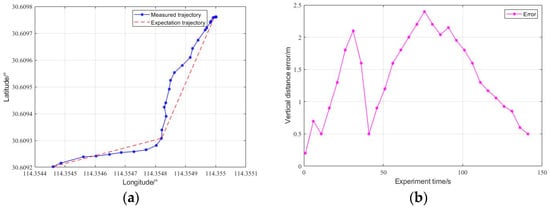
Figure 20.
Improved bending trajectory tracking experiment. (a) Folded trajectory; (b) track tracking error.
5.2.2. Triangle Tracking Experiment
The design process of the triangle trajectory tracking experiment is consistent with the folded line. The remote control platform sends the point information set in advance to the USV, which executes the automatic trajectory tracking control mode and follows the sent points in turn to complete the triangle trajectory tracking experiment.
Figure 21 and Figure 22 are the experimental data obtained before and after the improvement of the algorithm. The analysis of the experimental results shows that the total length of the track is 120.4 m, the maximum error in the experimental results before the improvement of the algorithm is 3.8 m, and the average error is 2.62 m. The maximum error of the improved algorithm is 2.7 m, and the average error is 1.53 m. The improved algorithm has higher control accuracy.
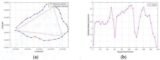
Figure 21.
Triangular trajectory tracking experiment before improvement. (a) Triangular trajectory; (b) track tracking error.
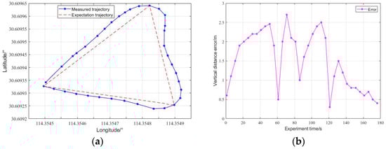
Figure 22.
Improved triangular trajectory tracking experiment. (a) Triangular trajectory; (b) track tracking error.
5.2.3. Quadrilateral Tracking Experiment
The trajectory tracking effect and error before the algorithm improvement are shown in Figure 23. The maximum error reaches 4.8 m and the average error is 2.35 m. The control effect of the improved algorithm is shown in Figure 24, from which it can be seen that the maximum error reaches 2.40 m and the average error 1.89 m, and the improved algorithm trajectory control effect is more excellent.
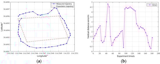
Figure 23.
Experiment on tracking quadrilateral trajectory. (a) Triangular trajectory; (b) track tracking error.
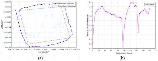
Figure 24.
Improved quadrilateral trajectory tracking experiment. (a) Triangular trajectory; (b) track tracking error.
5.3. Water Quality Test
With the help of the remote wireless network control platform and built-in trajectory tracking control algorithm, the unmanned boat with autonomous navigation capability for water quality testing, can effectively reduce the cost of manual testing and reduce the technical threshold of the operator. When the data measured by the sensors is in a stable state, the water temperature, turbidity, and pH data measured at this time are considered as the effective data of the track point.
In this paper, a pool was used as a water quality testing object scenario, while the upper platform preset eleven track points. Figure 25 shows the detection of track points which are tracked latitude and longitude sent down to the USV and which control the USV on these points in order of number tracking, tracking on the track points after the sensor in the case of stable readings to collect the point of water quality data in real time. Through the analysis of the water quality data stored in the background of the upper computer, a preliminary understanding of the distribution of water quality changes in the pool can be obtained.
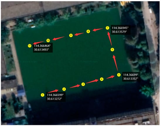
Figure 25.
Experimental water detection route.
Two valid data were extracted near the set track point to reflect the water quality around the point. The measured data were analyzed to obtain the linear distribution of water temperature, turbidity, and pH. Figure 26, Figure 27 and Figure 28 show the detection of water temperature, turbidity, and pH, respectively. So the initial task of water quality spot detection of the pool was completed. In this process, the use of the designed USV platform equipped with a water quality testing module combined with remote wireless network control platform, and USV built-in control algorithm finally realized automatic water quality testing. Through the analysis of the data measured at the spot, we can roughly know the water quality distribution of the pool within the vicinity of the set track. It is of a certain value for the practical applications such as aquaculture and water conservancy inspection.
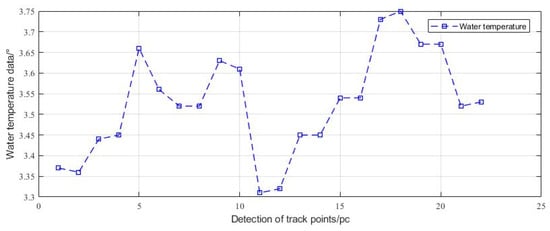
Figure 26.
Water temperature detection.
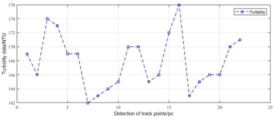
Figure 27.
Turbidity detection.
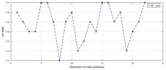
Figure 28.
pH test result.
5.4. Summary
Firstly, the traditional line-of-sight (LOS) guidance algorithm was introduced and its implementation principle was analyzed in conjunction with the USV trajectory tracking control requirements. Combined with the large deviation and steering problems in the actual situation of trajectory tracking, the track correction strategy and precise steering control strategy were proposed, respectively. By comparing the size of the corresponding track error before and after the algorithm improvement, the proposed improved algorithm was verified to have better trajectory tracking control. Finally, with the water quality testing hardware response characteristics and the test pool, which set a series of track points and fixed-point water quality testing, we achieved the autonomous water quality testing function.
6. Conclusions
The main work of this paper is as follows:
- The intelligent control system of the USV was designed from the perspective of low cost and small volume, which provides perfect experimental conditions for the subsequent experiments of remote manipulation and autonomous navigation motion control;
- In this paper, a mathematical model of the simplified planar motion of the unmanned ship was established to lay the foundation for the subsequent research. We combined the symmetrical two-motor structure of the unmanned ship and its type to establish a mathematical model of the motion of the two thrusters. Through simulation experiments, combined with the actual steering control, we derived the mapping relationship between rudder angle and motor speed;
- For the underlying motion control, the HSIC humanoid intelligent motion control strategy was introduced and compared with the PID control method for simulation, and the simulation verified the stability and feasibility of the algorithm;
- In view of the large deviation and steering problems of the line-of-sight (LOS) algorithm, the trajectory correction and precise steering control strategy was proposed, and the improved algorithm trajectory tracking accuracy and control practicality were verified by the designed and completed multi-point trajectory tracking experiments, and the autonomous water quality fixed-point detection function was realized.
There are also some shortcomings in this paper., such as the control system information acquisition and transmission mode are single, and the actual control process may have unstable transmission. There is a need to strengthen the sensor multi-data fusion and multi-redundancy communication design in the future. At the same time, for the trajectory tracking control algorithm design, there is no interaction with the water environment (such as autonomous collision avoidance, etc.), which will be studied in the next step.
Author Contributions
Y.X.: Conceptualization, Data curation, Formal analysis, Visualization; H.Z.: Writing–original draft, Investigation, Software; L.P.: Supervision, Funding acquisition, Project administration, Formal analysis; J.W.: Writing–review and editing, Validation, Resources, Methodology. All authors have read and agreed to the published version of the manuscript.
Funding
This research was funded by the Hainan Provincial Joint Project of Sanya Yazhou Bay Science and Technology City, China grant number (Grant No. 2021JJLH0036).
Institutional Review Board Statement
Not applicable.
Informed Consent Statement
Not applicable.
Data Availability Statement
Not applicable.
Conflicts of Interest
The authors declare no conflict of interest.
References
- Qiu, B.; Wang, G.; Fan, Y.; Mu, D.; Sun, X. Path Following of Underactuated Unmanned Surface Vehicle Based on Trajectory Linearization Control with Input Saturation and External Disturbances. Int. J. Control Autom. Syst. 2020, 18, 2108–2119. [Google Scholar] [CrossRef]
- Karaki, A.A.; Bibuli, M.; Caccia, M.; Ferrando, I.; Gagliolo, S.; Odetti, A.; Sguerso, D. Multi-Platforms and Multi-Sensors Integrated Survey for the Submerged and Emerged Areas. J. Mar. Sci. Eng. 2022, 10, 753. [Google Scholar] [CrossRef]
- Xu, C.; Hu, J.; Chen, J.; Ge, Y.; Liang, R. Sensor Placement with Two-Dimensional Equal Arc Length Non-Uniform Sampling for Underwater Terrain Deformation Monitoring. J. Mar. Sci. Eng. 2021, 9, 954. [Google Scholar] [CrossRef]
- Allen, J.; Iglesias, G.; Greaves, D.; Miles, J. Physical Modelling of the Effect on the Wave Field of the WaveCat Wave Energy Converter. J. Mar. Sci. Eng. 2021, 9, 309. [Google Scholar] [CrossRef]
- Storey, M.V.; van der Gaag, B.; Burns, B.P. Advances in On-Line Drinking Water Quality Monitoring and Early Warning Systems. Water Res. 2011, 45, 741–747. [Google Scholar] [CrossRef] [PubMed]
- de Sousa, J.B.; Andrade Gonçalves, G. Unmanned Vehicles for Environmental Data Collection. Clean Techn. Environ. Policy 2011, 13, 369–380. [Google Scholar] [CrossRef]
- Bonastre, A.; Ors, R.; Capella, J.V.; Fabra, M.J.; Peris, M. In-Line Chemical Analysis of Wastewater: Present and Future Trends. TrAC Trends Anal. Chem. 2005, 24, 128–137. [Google Scholar] [CrossRef]
- Greenwood, R.; Mills, G.A.; Roig, B. Introduction to Emerging Tools and Their Use in Water Monitoring. TrAC Trends Anal. Chem. 2007, 26, 263–267. [Google Scholar] [CrossRef]
- Scholin, C.; Doucette, G.; Jensen, S.; Roman, B.; Pargett, D.; Marin, R.; Preston, C.; Jones, W.; Feldman, J.; Everlove, C.; et al. Remote Detection of Marine Microbes, Small Invertebrates, Harmful Algae, and Biotoxins Using the Environmental Sample Processor (Esp). Oceanography 2009, 22, 158–167. [Google Scholar] [CrossRef]
- Matos, A.; Cruz, N. Positioning Control of an Underactuated Surface Vessel. In Proceedings of the OCEANS 2008, Quebec City, QC, Canada, 15–18 September 2008; pp. 1–5. [Google Scholar]
- Breivik, M.; Hovstein, V.E.; Fossen, T.I. Straight-Line Target Tracking for Unmanned Surface Vehicles. MIC J. 2008, 29, 131–149. [Google Scholar] [CrossRef] [Green Version]
- Lin, M.; Zhang, Z.; Pang, Y.; Lin, H.; Ji, Q. Underactuated USV Path Following Mechanism Based on the Cascade Method. Sci. Rep. 2022, 12, 1461. [Google Scholar] [CrossRef] [PubMed]
- Zhang, Y.; Liu, C.; Zhang, N.; Ye, Q.; Su, W. Finite-Time Controller Design for the Dynamic Positioning of Ships Considering Disturbances and Actuator Constraints. J. Mar. Sci. Eng. 2022, 10, 1034. [Google Scholar] [CrossRef]
- Borme, D.; Legovini, S.; de Olazabal, A.; Tirelli, V. Diet of Adult Sardine Sardina Pilchardus in the Gulf of Trieste, Northern Adriatic Sea. J. Mar. Sci. Eng. 2022, 10, 1012. [Google Scholar] [CrossRef]
- Huang, J.; Choi, H.-S.; Vu, M.T.; Jung, D.-W.; Choo, K.-B.; Cho, H.-J.; Nam Anh, P.H.; Zhang, R.; Park, J.-H.; Kim, J.-Y.; et al. Study on Position and Shape Effect of the Wings on Motion of Underwater Gliders. J. Mar. Sci. Eng. 2022, 10, 891. [Google Scholar] [CrossRef]
- Ntouras, D.; Papadakis, G.; Belibassakis, K. Ship Bow Wings with Application to Trim and Resistance Control in Calm Water and in Waves. J. Mar. Sci. Eng. 2022, 10, 492. [Google Scholar] [CrossRef]
- Wu, R.; Du, J. Adaptive Robust Course-Tracking Control of Time-Varying Uncertain Ships with Disturbances. Int. J. Control Autom. Syst. 2019, 17, 1847–1855. [Google Scholar] [CrossRef]
- Fang, Y.; Pang, M.; Wang, B. A Course Control System of Unmanned Surface Vehicle (USV) Using Back-Propagation Neural Network (BPNN) and Artificial Bee Colony (ABC) Algorithm. Procedia Comput. Sci. 2017, 111, 361–366. [Google Scholar] [CrossRef]
- Choi, W.; Kang, H.; Lee, J. Robust Localization of Unmanned Surface Vehicle Using DDQN-AM. Int. J. Control Autom. Syst. 2021, 19, 1920–1930. [Google Scholar] [CrossRef]
- Qi, Y.; Yu, W.; Huang, J.; Yu, Y. Model Predictive Control for Switched Systems with a Novel Mixed Time/Event-Triggering Mechanism. Nonlinear Anal. Hybrid Syst. 2021, 42, 101081. [Google Scholar] [CrossRef]
- Islam, M.M.; Siffat, S.A.; Ahmad, I.; Liaquat, M. Robust Integral Backstepping and Terminal Synergetic Control of Course Keeping for Ships. Ocean. Eng. 2021, 221, 108532. [Google Scholar] [CrossRef]
- Maurya, P.; Aguiar, A.P.; Pascoal, A. Marine Vehicle Path Following Using Inner-Outer Loop Control. IFAC Proc. Vol. 2009, 42, 38–43. [Google Scholar] [CrossRef]
- Min, B.; Zhang, X. Concise Robust Fuzzy Nonlinear Feedback Track Keeping Control for Ships Using Multi-Technique Improved LOS Guidance. Ocean. Eng. 2021, 224, 108734. [Google Scholar] [CrossRef]
- Gonzalez-Garcia, A.; Barragan-Alcantar, D.; Collado-Gonzalez, I.; Garrido, L. Adaptive Dynamic Programming and Deep Reinforcement Learning for the Control of an Unmanned Surface Vehicle: Experimental Results. Control. Eng. Pract. 2021, 111, 104807. [Google Scholar] [CrossRef]
- Kim, D.; Shin, J.-U.; Kim, H.; Kim, H.; Lee, D.; Lee, S.-M.; Myung, H. Development and Experimental Testing of an Autonomous Jellyfish Detection and Removal Robot System. Int. J. Control Autom. Syst. 2016, 14, 312–322. [Google Scholar] [CrossRef]
- Fossen, T.I. Guidance and Control of Ocean Vehicles. Doctors Thesis, University of Trondheim, Trondheim, Norway, 1999. Printed by John Wiley & Sons: Chichester, UK, 1999; ISBN 0-471-94113-1.. [Google Scholar]
- Ran, S.; Wang, N.; Pu, H.; Yin, C.; Wang, T.; Wang, T. Adaptive Point Stabilization Control of Two-Wheel Robot with Parameter Uncertainties Based on Human-Simulated Intelligent Backstepping Method. In Proceedings of the 2018 37th Chinese Control Conference (CCC), Wuhan, China, 25–27 July 2018; pp. 3915–3920. [Google Scholar]
- Qiu, B.; Wang, G.; Fan, Y. Predictor LOS-Based Trajectory Linearization Control for Path Following of Underactuated Unmanned Surface Vehicle with Input Saturation. Ocean. Eng. 2020, 214, 107874. [Google Scholar] [CrossRef]
- Fossen, T.I. Marine Control Systems–Guidance. Navigation, and Control of Ships, Rigs and Underwater Vehicles; Org. Number NO 985 195 005 MVA; Marine Cybernetics: Trondheim, Norway, 2002; ISBN 82-92356-00-2. [Google Scholar]
Publisher’s Note: MDPI stays neutral with regard to jurisdictional claims in published maps and institutional affiliations. |
© 2022 by the authors. Licensee MDPI, Basel, Switzerland. This article is an open access article distributed under the terms and conditions of the Creative Commons Attribution (CC BY) license (https://creativecommons.org/licenses/by/4.0/).