Abstract
The paper proposes a new method for the synthesis of spatial motion control systems of the AUV-leader and a group of AUV-followers during their cooperative movement in a desired formation. This system allows the provision of an accurate positioning of the followers relative to the leader using information received with a low frequency only from their onboard video cameras. To improve the accuracy of the created system it proposes a method of estimation of the parameters of the movement of the AUV-leader (its speeds and accelerations) to predict its movement relative to the AUV-follower in the time intervals between the updates of information received from video cameras.
1. Introduction
Now, the use of groups of autonomous underwater vehicles (AUVs) is the most promising way to increase the efficiency of underwater operations performed by AUV [1]. This is especially important for the operations of bottom mapping, searching, the transportation of underwater objects, and others. The strategy “leader-followers” is one of the most popular approaches for AUV cooperative control. This strategy supposes that one AUV is a leader, and the others are followers. The AUV-leader has full information about the mission and plans the trajectory, and the AUV-followers move the leader and keep a setting position relative to the leader [1].
Many approaches to the synthesis of control systems for the formation control of groups of robots for various purposes are known. These approaches are based on various methods of the control theory and make it possible to hold the position of robot-followers in the desired formation, while considering the uncertainty of their parameters and the influence of external disturbances [2,3,4,5,6]. At the same time, it is assumed that all the robots of the group should determine its position and receive information about the position and movement parameters of the leader. In the case of AUV, the specified information must be received through acoustic communication channels [7,8,9,10], which have a limited bandwidth and long delays in data transmission.
Various approaches are proposed to consider the features of these communication channels when implementing AUV formation control systems. To reduce the impact of the limited bandwidth of these communication channels, the use of an extended Kalman filter is proposed in [11]. Using this filter, the AUV-followers predict the position of the AUV-leader based on data on its speed and position obtained with a low frequency. However, the implementation of this approach requires the matching navigation systems of the AUV-followers and the AUV-leader for the correct determination of the AUV-followers’ position relative to the leader in the absolute coordinate system (ACS). To solve this problem, the methods described in [12,13,14] can be used. However, their use can significantly complicate the synthesis of AUV cooperative control systems.
Other solutions that do not require the use of data about the AUV-leader and AUV-followers’ coordinates in ASCs are the formation control methods based on data about position of the AUV-followers relative to the leader, obtained using their onboard sensors [15]. In the work of [16], a formation control method of AUVs is proposed. In this method, the AUV-leader sends to the AUV-followers information about its current speed, the yaw angle, and yaw angular velocity via acoustic communication channels. At the same time, the followers, with the help of onboard acoustic sensors, determine the distance and direction to the AUV-leader. That allows the calculation of the current deviation of the follower from a desired position in the formation. However, these communication channels used for data exchange between AUVs have low a bandwidth and long delays in data transmission, which do not allow the AUV-followers to move safely and accurately at a small distance from each other. One of the ways to solve these problems is the use of AUV formation control systems based on data received from their onboard video cameras. It allows the exclusion of the data exchange through the acoustic communication channels and the matching of the navigation systems of the AUV-leader and the AUV-followers. In addition, the use of the data about the position of the AUV-followers relative to the leader, obtained from onboard video cameras, makes it possible to not use expensive hydroacoustic navigation systems on board the AUV-followers.
It should be noted that the main difficulty with using video information is the relatively small distance at which the onboard video camera can operate. Usually, depending on the state of the underwater environment, this distance is 5–15 m [17]. However, there is a large class of tasks for which such distances between the AUVs of the group are the working distances. For example, geotechnical survey can be attributed to these tasks. When performing these operations, the AUV group implements a field of hydrophones, where they must accurately hold the specified distances between themselves, which equal a few meters [18]. Also relevant is the task of creating an AUV assistant [19], which should move behind the diver at a given short distance. Currently, video information is widely used to create AUV automatic docking systems [17,20,21]. In these systems, the position and orientation of the AUV relative to the docking stations is determined by means of light beacons installed at these stations. At the same time, during the docking process, the linear and angular velocities of the AUV relative to the stations are determined only by the AUV’s own movement as the stations are stationary. However, when AUVs are moving in a group, the speed and direction of the AUV-leader’s movement may change unexpectedly, especially when the leader bypasses obstacles. This requires an additional estimation of all the motion parameters in the presence of video information. Moreover, the data about the position and orientation of the AUV-followers’ relative leader, formed by means of video information, can be updated slowly, which greatly reduces the accuracy of the AUV-followers’ movement as this cannot allow the generation of the control signals with high frequency. In [22], a method for solving this problem is proposed for industrial manipulators tracking a moving object using a video camera. In this method, a Kalman filter and a special predictor are used for estimating the speed of a moving object, which can compensate for the delays that occur in the process of obtaining the required estimates. The position of the video camera and the position of the object are formed in the ACS, which allows the prediction of the movement of the object independently of the movement of the manipulator. However, the position and orientation of the AUV-follower’s relative leader depend on the spatial movement and orientation of the followers themselves, and this factor requires additional consideration to generate control signals for the AUV-followers.
In [23], the method for the control of the AUV-followers’ movement based on the information received from their onboard video cameras is proposed. However, in this work, the estimation of the AUV-leader’s speed relative to the follower was carried out using numerical differentiation of the estimation of the AUV-leader’s position, which significantly reduced the accuracy of this estimation and, consequently, the control accuracy. Moreover, the proposed method assumed that the AUV group moves only in the horizontal plane, and it cannot be used in the case when the AUV leader moves in space, such as when holding a given height above a bottom with difficult relief.
Thus, in this paper the set task is to develop a control system for the AUV-follower which provides the high-precision holding of a desired position of the AUV-follower relative to the AUV-leader based on data received from the AUV-follower’s onboard video camera. The approach proposed in the paper is based on an estimation of the position and movement parameters (speed and acceleration) of the target point, which sets the desired position of the AUV-follower relative to the AUV-leader. This estimation is performed by means of a data series received from the onboard video camera of the AUV-follower for a certain period. The position of the target point is formed as a polynomial time function describing the change of the target point coordinates relative to the AUV-follower. The obtained functions are used to predict the movement of the target point in the time interval between the updates of the data received from the video camera, with consideration of the AUV-follower’s own movement. These estimates are used to generate program signals, which are worked out from the AUV-follower’s onboard control system, which considers the uncertainties of the parameters of the slave.
This approach will ensure the movement of AUV-followers without the use of acoustic communication channels and hydroacoustic navigation systems. It will reduce the cost of using AUV groups to perform various underwater operations requiring the movement of AUVs in a group with relatively short distances between AUVs (bottom photography, environmental monitoring, seismicity studies, etc.).
The contributions of this paper are the following.
1. A method of estimating the vectors of the position, speed, and acceleration of the target point, which determine the position of the AUV-follower in the formation, relative to this AUV-follower. This estimation is based on the series of measurements of the position and orientation of the AUV-leader relative to the follower and is formed as polynomial time functions. This approach makes it possible to reduce the influence of the errors that occur when measuring the position and orientation of the AUV-leader, as well as to reduce the delay in determining speeds and accelerations compared to the traditional methods.
2. A method for predicting the movement of the target point of the AUV-follower in the time interval between the updates of data received from the video camera, with consideration of the AUV-follower’s own movement. This makes it possible to significantly increase the frequency of the updating information about the current deviation of the follower from the desired position in the formation. It can provide the possibility of using high-precision control systems.
The main notations used in the article are described in Table 1.

Table 1.
List of notations.
2. Problem Definition
The paper considers the group of AUVs, consisting of the AUV-leader and the AUV-followers. The leader has information about the mission and plans the trajectory of movement in the process of its performance. Each AUV-follower moves for the leader and holds its desired position in the formation (point in Figure 1).

Figure 1.
Scheme of leader–follower movement.
The desired position of each AUV-follower is set in the coordinate system (CS) , the beginning of which coincides with the CS joined with the AUV-leader, and the zLR axis is parallel to the z axis of the absolute CS (ACS). This ensures that the desired positions of the followers relative to the leader in the vertical axes do not change when the leader moves in space with a change of the roll and pitch angles.
It is assumed that each follower does not receive data about the movement of the leader transmitted via acoustic communication channels, and the AUV-followers do not have information about their position in the ACS. Each follower has onboard inertial sensors that allow the measurement of the orientation angles, linear and angular velocities, and accelerations of the AUV-follower. Several light beacons are installed on the AUV-leader. Their locations relative to the center mass of the leader is known and have the coordinates B = (B1, B2, …, Bn), where Bi = (xbi, ybi, zbi)T are the coordinates of the i-th beacon in the AUV-leader’s CS. These beacons have characteristics that make it possible to identify them in the image received from the video camera and to calculate their pixel coordinates in this image. These pixel coordinates form a vector are the pixel coordinates of the i–th beacon in the image.
The model for converting the three-dimensional coordinates of a point existing in the field of view of a video camera into pixel coordinates, considering the effects of distortion, has the form [24]:
where cp = (fx, fy, cx, cy) is the vector of the internal parameters of the video camera; U = (k1, k2, k3, u1, u2) is the vector of the parameters of the radial and tangential distortion of the camera; is the vector of the coordinates of a point in the camera CS; is the vector of the pixel coordinates corresponding to a point . The internal parameters of the video camera and the distortion parameters are determined using standard calibration procedures.
It is assumed that the updating frequency of the frames from the onboard video camera may be insufficient for the implementation of the high-precision motion control systems of the AUV-followers. The dynamics of the AUV-follower in its body-fixed CS (BCS) are described by the equations system [25]:
where ; is an AUV inertia matrix; is a matrix of added mass and moment inertia; is a matrix of Coriolis and centripetal forces and torques; D is a matrix of hydrodynamic forces and moments; is a vector of hydrostatic forces and torques; is a vector of the AUV orientation angles in the ACS; is a vector of propulsion forces and torques in the AUV BCS; and is a vector of linear and angular velocities in the AUV BCS.
The matrix of Coriolis and centripetal forces and torques is described by the expressions [25]:
where , , and operator is described by the expressions:
The matrix of hydrodynamical forces and torques is diagonal, and its entries have following view [25]:
where d1i and d2i are the hydrodynamic coefficients.
The vector of the hydrostatic forces and torques has the following form [25]:
where Wa is the gravity force; Ba is the buoyancy force; , , and ; are the coordinates of the center of gravity (CG) in the AUV BCS; are the coordinates of the center of buoyancy (CB) in the AUV BCS.
The AUV parameters are not known exactly and can change, for example during the transportation of cargo which is unknown in advance. Because the parameters M, d1, and d2 enter into Equations (2)–(4) linearly, the AUV dynamic can be described in the following form:
where are the forces and torques that occur when the AUV is moving and depend on the nominal values of the AUV parameters; are the forces and torques that occur when the AUV is moving and depend on the uncertain or variable part of the AUV parameters; are the nominal values of the AUV parameters; and are the uncertain or variable parts of the AUV parameters. The matrixes are calculated by Expressions (3) and (4) with the use of .
It is supposed that the following conditions are satisfied for the matrixes and , and the entries of matrix , and the vectors :
where , , , and , are the estimations of the maximum deviations of the AUV’s parameters and the entries of the corresponding matrixes from their nominal values.
The following task is set in the paper with consideration of the models describing the AUVs and their video cameras. Based on the information about the pixel coordinates of the light beacon located on the AUV-leader, it is to develop a method for determining the position and speed of a target point movement, which sets the desired position of each follower relative to the leader. The information about the target point movement must be generated with a given discreteness, regardless of the frequency of the updating frames from the onboard video cameras. A control system of the AUV-follower should be synthesized that ensures a given accuracy of the positioning of the AUV-follower with consideration of the unknown vales of the AUV-follower’s parameters described by the Expression (6).
3. The Formation of the Position, Orientation, and Speeds of Target Point Relative to the AUV-Follower with a Desired Period
To solve this problem, we propose a control system, the diagram of which is shown in Figure 2. From this diagram, the formation of the control signal of the AUV-follower includes several steps.
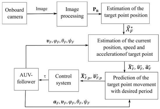
Figure 2.
The diagram of AUV-follower control system.
Initially, the AUV-leader light beacons are allocated on the frames received from the onboard video camera using standard image-processing algorithms, and the PB vector of their pixel coordinates is formed. This vector is used to determine the position and orientation of the leader relative to the follower and for the calculation of the target point position of each AUV-follower in its BCS. Information about contains inaccuracies arising due to errors in determining the pixel coordinates of the light beacons and the parameters of the video camera. These inaccuracies lead to errors in determining the velocity and acceleration of the target point movement of the AUV-follower in the BCS, and as a result, this reduces the control accuracy of the AUV-follower movement.
To improve the control accuracy, the forming of special polynomial functions approximating the changing coordinates of the target points of the AUV-follower is proposed. These functions allow the prediction of the changes of these coordinates at the period of the data update from the onboard video cameras. Moreover, an analytical description of the motion of point is formed, which is used to determine the changes of its position velocities with consideration of the AUV-follower’s own movement. The estimations and are formed with a necessary period, which is independent of the update period of the data from the onboard camera.
After the formation of the position and speed of each target point relative to the corresponding follower, the program signals of movement are calculated, considering the kinematic features of this follower. These program signals are worked out by the AUV control system, which provides the desired accuracy of the AUV-follower’s movement relative to the leader with any changes in their parameters in the ranges (6).
Next, we will consider sequentially the implementation of all the stages of the system.
3.1. The Estimation of the Positions and Movement Parameters of the Target Points of Each AUV-Follower Based on Data Received from Their Onboard Video Cameras
At the first stage, the position and orientation of the AUV-leader relative to the follower are determined using the vector PB of the pixel coordinates of the beacons, the vector cp of the internal parameters of the video camera, and the vector U of the distortion parameters obtained using standard calibration procedures.
The pixel coordinates of the i-th light beacon and the position and orientation of the AUV-leader in the CS of the camera, with consideration of model (1), are determined by the equation system:
where is the AUV-leader position in the CS of the AUV-follower camera; is the vector of the AUV-leader orientation angles in the CS of the AUV-follower camera; and is the rotation matrix of the leader CS relative to the CS of the camera.
System (7) contains six unknown variables included in the vectors and . To determine these variables, at least three light beacons must be placed on the AUV-leader.
System (7) is essentially nonlinear and cannot be solved analytically. Therefore, to determine the values of and , it is advisable to use the Levenberg–Markgvard numerical optimization method [26], which has sufficiently fast convergence and relatively low computational complexity. This will allow it to be used in the onboard control systems working in real time.
The cost function for estimating and has the following form:
where is the estimation of the pixel coordinates of i-th beacon calculated by the means of Equations (1) and (7) and the current estimation of the unknown vector .
For using the Livenberg–Markgwardt method, it is necessary to calculate the matrix of the first partial derivatives of the vector according to the estimated parameters [26]. Due to the complexity of Equation (7), analytical expressions for calculating the matrix G contain many operations. To simplify the calculation of G, it is better to use the numerical method of calculating derivatives described in [27]. Using this method, the matrix is formed as:
where ih is the small imaginary value, which is an increment of the corresponding component of the vector , while all other arguments of the function remain unchanged; Im is the imaginary part.
The vector G (9), calculated for the current value of the vector , is used to determine the increment of this vector using the expressions [26]:
where k is the iteration number; I∈R6×6 is the unity diagonal matrix; μ(k) is the step of adjusting; and 0 < η < 1 is the coefficient of step changing.
The vector is set in the onboard video camera CS and used for calculating the position of the target point relative to the AUV-follower. This calculation is performed in two stages.
In the first stage, the position and orientation of the leader in the CS is calculated. The beginning of the CS coincides with the beginning of the AUV-follower BCS, and the axis is parallel to the z axis of the ACS (see Figure 1). These values are calculated using the expressions:
where are the vectors of the position and orientation angles of the AUV-leader in the CS ; is the rotation matrix of the camera CS relative to the AUV-follower BCS; is the rotation matrix of the AUV-follower BCS relative to the CS ; is the rotation matrix of the AUV-follower BCS relative to the ACS; is the rotation matrix around the z axis of the ACS; is the coordinate vector in the AUV-follower BCS; is the entry of orientation matrix of the AUV-leader in the CS .
The estimation of the position of the target point for the AUV-follower relative to the AUV-leader in the CS is determined by the expression:
where is the desired position of the AUV-follower in the CS .
For the high-precision movement of the AUV-follower in conditions of the uncertainty and variability of their parameters, it is necessary to use high-precision control systems, the implementation of which requires a high-frequency updating of the control signals.
However, as the update of the vector , as a rule, occurs with a low frequency, it is necessary to form a control signal with an increased frequency at intervals between the updates of the data coming from the video cameras to provide the required precision of the control. To do this, the changes of should be predicted using information about the speeds and accelerations of these changes. However, it is not possible to predict changes in the vectors precisely enough, considering the significant errors in calculating the pixel coordinates of the light beacons and the inaccuracies in determining the parameters of the onboard video cameras. This leads to a reduction in the control precision of the AUV-follower. To eliminate this drawback, the use of the following approach for the improvement of the estimations of vector and its speeds and accelerations is proposed (see Figure 3).
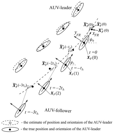
Figure 3.
The measurement series for defining the position and parameters of movement of target point.
This figure shows the positions of the AUV-leader and one AUV-follower at the four points in time (at the moment of updating data from the video camera). The calculated positions and orientations of the AUV-leader differ from the real ones. This leads to errors in determining the positions of the target points for the current positions of the follower (black circles near the dashed line are the true positions of the target points, and the white ones are positions calculated using Expressions (7)–(12)).
To reduce the influence of these errors on the precision of the AUV-followers’ control systems, it is required to include in these systems information about the speeds and accelerations of the movement of these target points [25]. This information can be obtained by approximating the sequence of the previously calculated points by a smooth polynomial function. As result, this sequence can be described by the function , graphically depicted in Figure 3 by a dashed line, where is the vector of coefficients of the polynomial function, N is the specified order of the polynomial. In this case, the points (corresponding to the gray circles on the dashed line) correspond to new estimates of the position of the point at the time .
It is better to use the least squares method to calculate the vector λ. This method minimizes the sum of the distances between the points и . Therefore, the obtained analytical description of the approximating curve (dashed line in Figure 3) describes the movement of the target point .
As the vectors are calculated by taking into account the corresponding positions of the AUV-follower, the sequence will depend not only on the movement of the AUV-leader, but also on the follower’s own movements relative to the leader. This complicates the prediction of the movement of points and requires consideration of the previous movement of the follower. The positions of the points should be recalculated relative to the current position and orientations of the BCS of the follower to facilitate the solution to this problem. This allows the separation of the movements of the points , determined by the movement of the AUV-leader and the movements of the AUV-followers themselves. To do this, it is necessary to consider the speed and orientation of the followers at the appropriate time moments.
This approach allows the performance of the following:
- -
- To reduce the calculation errors of by smoothing the sequence of the values of on a given period by means of a polynomial function;
- -
- To estimate the values of the elements of the vectors of position , the velocities , and the accelerations of the movement of the point without entering additional delays;
- -
- To obtain an analytical description of the movement of the point , which is used to predict its movement relative to the follower in the time interval between updating data from the onboard camera.
It is obvious that approximation errors may appear with a sharp change in the direction of movement of the AUV-leader, such as, for example, when the leader bypasses obstacles that unexpectedly appear in the way of its movement. However, it will be shown later in the simulation that these errors do not lead to significant deviations of the followers from their desired position.
Below is a description of the proposed method.
Let us assume that during the movement of the AUV group, for each follower the array Ω of size M + 1 is formed, and the following data are stored with period in each of its elements:
- -
- The vector of the coordinates of the target point of the AUV-follower in the CS (Figure 3);
- -
- The vector of the linear speed of the AUV-follower in its BCS;
- -
- The vector of the orientation angles of the AUV-follower in the ACS.
As a result, the i-th element of array contains the vectors where i = 0 corresponds to the current time , and i = M corresponds to time .
If new data are received from the onboard video camera, then the array Ω is updated: outdated data from the end of the array Ω are removed, and new ones are added to the beginning.
The vector stored in the array Ω, corresponding to the position of the target point at the i-th moment of time, are recalculated into the CS at the time corresponding to i = 0 (see Figure 3). This recalculation occurs iteratively from the first element of the array Ω to the last one according to the formulas:
where are the coordinates of the target point in the time moment in the CS when t = 0; is the position of the AUV-follower in the time moment in the CS when t = 0 (;
is the rotation matrix of AUV-follower BCS with respect to the ACS [25]; the indexes correspond to the elements of vector ; are the values of the yaw angle in time moments 0 and respectively.
This procedure forms a new array of , containing data on the time changes of the vectors of the coordinates of the target points relative to the current positions of the SC . As a result, the sequence of target points in array can be approximated using polynomials of order N. That is, changes in the coordinates , , of the vectors in time can be described using the expressions:
where are the initial values of the coordinates of the target point; are the initial values of the speeds of these coordinates; a are the initial values of their accelerations; kx1,…, kxN−2, ky1,…, kyN−2, kz1,…, kzN−2 are the coefficients of the polynomial approximant.
Furthermore, to reduce the description, we consider the method of determining the coefficients of the polynomial (14) only for the coordinate . The coefficients for the other two polynomials are determined similarly. It is better to use the least mean squares method to determine the values . Let us rewrite the equality (14) in the matrix form:
The measurement sequence is set by vector S:
The form of vector S allows the determination of the first three coefficients of the polynomial (15), which coincides with the estimations of the values of the vector and its speeds and accelerations at the current time. This allows them to be used immediately in further calculations without additional transformations.
One can write, with consideration of Expressions (15) and (16):
where , is the vector of the coefficients of the polynomial.
The estimate of the coefficient vector λ with consideration of (17) will be calculated by the formula [28]:
If the period of updating the data into the vector S is constant, then the matrix is constant too, and it can be calculated in advance. This significantly reduces the computational complexity of the created algorithm. The use of the proposed algorithm requires the choosing of the size M of the array Ω and the order N of the approximating polynomial.
The value of N determines the accuracy of the approximation and depends on the types of trajectories of the AUV-leader. The higher the order of the approximating polynomial, the more accurate the estimation of the process of changing the coordinates of the target point will be, but less noise will be suppressed in the estimates of the velocities and accelerations. As most of the trajectories of the AUV can be described by curves of the second or third order, the value N can be assumed to be equal to 3 or 4.
The more data are used for the approximation, the more accurate are the given estimates until the type of trajectory of the AUV-leader does not change, but with sharp changes in the trajectories of the leader, the errors also increase. In addition, the large amount of data increases the computational complexity of the proposed algorithm. Therefore, the data series used for the approximation should be chosen for a duration of several seconds because the trajectory of the AUV-leader during such a time interval cannot change significantly.
Expressions (13)–(18) estimate the vectors positions, speeds, and accelerations of the movement of the target points for the follower at the current time. They are set in the CS .
These estimates do not consider the real movements of the follower when forming input signals for their onboard control systems. At the same time, these estimates can be used at the next stage, which consists of the prediction of the movements of the target points in the time intervals between the updates of data from the video cameras, with consideration of the real movements of the AUV-follower.
3.2. The Prediction Algorithm of Changing Position, Speed, and Accelerations of Target Point Movement
During the process of prediction, we will assume that changes of the positions of the target points relative to the positions of the follower at the time of the last receipt of data from the video cameras are described by the expression:
In Expression (19), there are no coefficients at high degrees of the approximating polynomial (15) as the prediction time intervals are rather small, and the main influence in the polynomial will be exerted by its first terms.
The coordinates of the target point in the CS , with consideration of the AUV-follower’s movement, are defined by expression:
where ; is the increment of the yaw angle of the AUV-follower from the beginning the prediction process, and is the follower’s movement from the beginning of the prediction process. The value is calculated by the formula:
where is the time interval of the prediction.
Differentiating Equation (20), we obtain:
where ; , .
Differentiating Equation (21), we obtain:
where are matrixes of the elementary rotations around the axes of the ACS.
In Expressions (21) and (22), the derivatives of the angles are used, which depend on the angular velocities measured by the onboard sensors of the AUV-follower, using the following expression [22]:
Considering the presence of moments of stability of the AUV, it is assumed that . So, we can simplify the calculations in Expressions (21) and (22) by using the following expressions:
Equations (20)–(22) are used to estimate the speeds and accelerations of the target points relative to the AUV-follower in the time intervals between updating the data about the current position and the orientation of the AUV-leader.
The prediction of changes in the coordinates when considering the current movement of the follower is proposed to be performed using a Kalman filter algorithm. Its block diagram is shown in Figure 4.
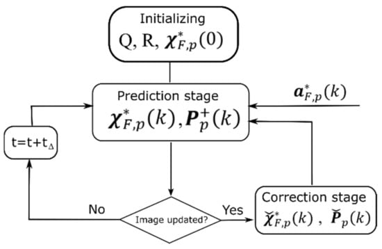
Figure 4.
The block diagram of Kalman filter for prediction of the target point movement relative to the AUV-follower.
At the initialization stage of this algorithm, the initial values of the covariance matrices , , are set. The initial values of the filter state vector , containing estimates of the speed and the position of the target points relative to the follower, are usually assumed to be zero.
After initialization, the main filter cycle works, which contains two stages: the prediction stage, where the positions and speeds of the movement of the target point relative to the follower are estimated with a desired period, and the correction stage, where the previously predicted values are corrected based on the data received from the onboard video cameras.
The following expressions are used at the prediction stage:
where ; ; is the period of calculation of the predicted value of vector ; is the covariation matrix, calculated at the prediction stage.
It can be seen from (23) that the input signal for the model is the acceleration vector of the target point, obtained based on Expression (22).
The prediction stage continues until the updated data is received from the onboard video camera. Vector is the estimation of the error of the position and speed of the AUV-follower and is used to generate the control signals for their movements.
After updating the data from the video camera, the correction stage begins, in which the previously predicted values are corrected using the latest measurements.
The measurement model has following form:
where is the vector of the current estimations of the position and speed of the target point relative to the AUV-follower.
This correction occurs by the following expressions:
where , is the state vector and the covariation matrix corrected by means of the new data received from the onboard camera.
After the correction, the prediction stage begins, in which the values of , are used as the initial values of the state vector and the covariance matrix.
After determining the errors of the positions and speeds of the follower, and considering its movement, these errors are used to generate the control signals.
4. The Synthesis of AUV-Follower Control System
The AUV-follower must move oriented towards its target point so that this point is on the axis of the BCS that coincides with its longitudinal axis. So, the desired values of the orientation angles of pitch and yaw and the rate of their change are calculated using the formulas:
where are the rate of change of the desired values of angles and . When the AUV-follower is in a given neighborhood of the target point, the values of the desired angles of its orientation are equal to .
The control signals of the AUV-follower are set in the BCS, and the positions of their target points are formed in the CS . Therefore, the movements of the follower, considering the models in (2), can be described by the equations:
where is the vector of the desired speed of the AUV-follower in the CS ; is the vector of error of the orientation angles; is the vector of the desired speed of the follower; .
Multiplying the first equation of system (27) by the matrix , we obtain
where , are the derivatives of the errors of the linear and angular speeds in the BCS of the follower, and are the vectors of desired linear and angular speeds in the BCS of the follower.
To control the movements of the follower, a combined control system was used. This control system consists of a nonlinear controller that forms the thrust , which ensures high accuracy of the follower movement when its parameters have the nominal values, and a sliding controller that forms the thrust , which compensates for the deviations of the follower parameters in the ranges (6) [29]. At the same time, the total thrust of the follower forms by the following expression
The nonlinear controller has the following form [26]:
where is the diagonal matrix of the positive coefficients; .
The sliding controller has the following form:
where ; is the diagonal matrix of the positive coefficients.
Let us define the following Lyapunov function . The derivative of V, with consideration of (2), has the following form:
Substituting Expressions (28)–(31) in (32), and considering the model (5), we obtain:
As [25] and , to then fulfill the condition the coefficient was chosen in accordance with the inequality
where is the acceptable dynamical error of control.
The variables and E for the synthesis of the control law (29)–(31) are formed using Expressions (20)–(25).
It is shown below that the synthesized control law (29)–(31), (34) provides the AUV-follower with the desired dynamic properties for any changes in its parameters in the ranges (6).
5. The Simulation Results
To check the features of the operation of the proposed system, including Expressions (18), (22)–(25) for predicting the movement of the target point and the control system (29), (30), and (34), the mathematical simulation was carried out. During this simulation the AUV-leader moved along the spatial trajectory.
The simulation was carried out using the CoppeliaSim environment, which allows us to simulate the work of the different robotic systems and their equipment in three-dimensional scenes. In this environment, the AUV-leader with light beacons installed on its body and the AUV-follower with an onboard video camera mounted on it were described. The work of the camera simulated in this environment. The image of the leader from the onboard camera of the follower was transmitted to an external program for further processing using Expressions (7)–(11). The movements of the leader and the follower and the work of the proposed system were studied in this external program. The calculated positions and orientations of the AUV-leader and follower were transferred to the CoppeliaSim environment to place their models three-dimensionally in the calculated positions with the calculated orientation.
The dynamics of the AUV-follower during simulation were described by a system of differential Equation (2), with the following nominal parameters [29]: , d1 = (18 Ns/m, 105 Ns/m, 105 Ns/m, 20 Nms, 80 Nms, 80 Nms), d2 = (18 Ns2/m2, 105 Ns2/m2, 105 Ns2/m2, 20 Nms2, 80 Nms2, 80 Nms2), , MA = (15 kg, 185 kg, 185 kg, 5 kgm2, 9.6 kgm2, 9.6 kgm2). These parameters are used for the synthesis of the control system (29)–(34). It is supposed that the deviations of the AUV-follower’s parameters have the following values: , =(9 Ns/m, 50 Ns/m, 50 Ns/m, 10 Nms, 30 Nms, 30 Nms), = (9 Ns2/m2, 50 Ns2/m2, 50 Ns2/m2, 10 Nms2, 30 Nms2, 30 Nms2).
The parameters of the control system have the following values: K .
The update period of the data received from the onboard video camera is 0.1 s. The prediction of the movement of the target point was carried out with a period of 0.001 s. The parameters of Expressions (11)–(18) for the estimation of the motion parameters of the target point had the values: N = 4, M = 50
During simulation, the AUV-leader moved in the ACS along the trajectory consisting of two parts. The first part corresponded to the movement of the leader along a straight line (m), y = 0 = const (m), and z = 1.2 = const (m), with a constant speed of 1.2 m/s. The second part of the leader’s trajectory was described by the equations . During the simulation, the longitudinal axis of the AUV-leader was always oriented along the trajectory of its movement. The projection of this complex trajectory onto a horizontal plane is shown in Figure 5, where the dotted curve is the trajectory of the leader movement, and the solid gray one is the desired trajectory of the follower movement. The vector defining the desired position of the follower in the AUV-leader BCS was following . The use of these trajectories for the simulation allows the investigation of the efficiency of the proposed system (11)–(18), (22)–(25), when the type of the AUV-leader trajectory is changed.

Figure 5.
The desired trajectories of AUV-leader and AUV-follower.
Two studies of the proposed prediction algorithm (Equations (18) and (22)–(25)) and the combined control system, including the nonlinear controller and a sliding controller defined by Equations (29), (30) and (34), were conducted.
In the first study, it was assumed that the current position and orientation of the AUV-leader were known exactly (they were not calculated using Expressions (7)–(11) from the images of the leader’s beacons received from the video camera). This made it possible to estimate not only the quality of the proposed prediction algorithm, but also the impact of possible prediction errors on the accuracy of the control of the AUV-follower’s movement.
In the second study, the position and orientation of the leader were calculated using Expressions (7)–(11), based on the images received from the CoppeliaSim environment. This study made it possible to evaluate the quality of the entire synthesized system using the data obtained after the image processing.
The results of the first study are shown in Figure 6. In this figure, the gray curves show changes in the coordinates and speeds of the target point moving along the program trajectory of the follower (gray curve in Figure 5), in the CS. The black curves show the estimates of these coordinates and velocities in this CS, calculated using Expressions (18), (22)–(25).
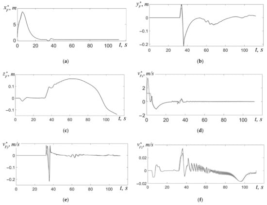
Figure 6.
The changing estimated and true values of coordinates ((a) is the ; (b) is the ; (c) is the ) and speeds ((d) is the ; (e) is the ; (f) is the ) of target point in the CS .
Before starting the movement in the initial position, the main axes of the leader and the follower coincide with the axes of the ACS; the array Ω is filled with zero values; the coordinates of the AUV-leader in the ACS are (3; 0; 1.2); and those of the AUV-follower are (−1.5; −6; 1.2). That is, the follower in the initial position was specially placed on the axis further from its program position relative to the leader, and the coordinates of the and the remained the same. Moreover, in the simulation, the movement of the AUV-follower began 4 s after the start of the movement of the leader. During this time, the position of the program point on the coordinate changed from 3 m to 7.8 m (see Figure 6a). This was conducted to check the accuracy of the system’s recovery of the required program position of the follower relative to the leader in the case of external disturbances.
The initial error between the target point and the AUV-follower (see Figure 6a) along the axis was worked out by its control system up to 0.2 m by the time of t = 28 s and did not increase further. During this time, the speed of movement of the target point relative to the follower along the axis (see Figure 6d) varied from 1.2 m/s (gray curve) to −1.1 m/s (at the stage of acceleration of the follower). Then, the changes in this speed did not exceed 0.02 m/s, which indicates the synchronization of the movement of the AUV-leader and the AUV-follower.
Negative values of the speeds in Figure 6d–f mean that the follower moves faster than the leader by the corresponding coordinate, approaching the target point, and the positive ones indicate that it moves slower than the leader, moving away from the target point.
From Figure 6a,d, it is seen that the prediction of the changes in the coordinates and the speed of the target point along the coordinate occurs with significant errors during the 6 s after the start of the slave movement. It takes place until the array Ω is filled with the data necessary for the correct operation of Expressions (18), (22)–(25). After filling this array, the deviations of the predicted position of the target point from its real position in the coordinate do not exceed 0.02 m, in the coordinate—0.002 m, and in the coordinate—0.01 m. This is quite enough for the high-quality control of the follower.
The analysis of the features of the system operation showed (see Figure 6c) that at the initial stage of movement, short-term deviations of the target point along the coordinate may occur. This is explained by the interactions between some degrees of freedom of the AUV, when acceleration along the x-axis of the BCS leads to the appearance of a torque along the pitch angle and the displacement of the AUV-follower along the axis. However, the interaction is quickly compensated for by the control system of the follower.
At the moment of changing the type of trajectory of the AUV-leader (t = 32 s in Figure 6) in the CS , the error between the true and predicted values of the coordinates and speeds of movement of the target point appears. This is due to the fact that not all the data contained in the array Ω (see Section 3.1) correspond to the new trajectory of the AUV-leader. However, this error is quickly (in a few seconds) worked out by the system. Studies have shown that the described effect occurs only with a sharp transition from a rectilinear to a curved trajectory. If these transitions are smoothed, then the described effect is weak.
Thus, the presented simulation results generally confirm the possibility of ensuring the high-precision movement of the AUV group with the help of the proposed control system, if the AUV-leader moves with a speed of up to 1.4 m/s, even with a long period (0.1 s) of updating the data about its position relative to the followers.
Figure 7 shows the control signals generated by the system (29), (30), and (34) by three degrees of freedom when using Expressions (18), (22)–(25) for prediction of the movement of the target point, which are obtained with accurate information about the position and orientation of the AUV-leader.
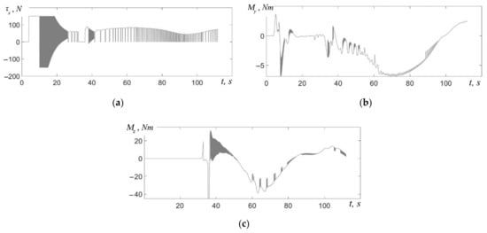
Figure 7.
The changes of control signals of AUV-follower: (a) is the ; (b) is the ; (c) is the .
Although the updating period of the data about the position and orientation of the AUV-leader is 0.1 s, the control signals (due to the use of a system with a sliding controller) are updated 100 times faster. Thus, the control system (29), (30), and (34) provides the required accuracy of the movement of the AUV-follower. At the same time, at the initial stage of movement (from 0 c to 32 s), the main control signal is formed by the xF coordinate (see Figure 7a) to work out in a sliding mode a large initial error between the follower and the target point. Additionally, at the moment of 32 s, the resulting large errors are also successfully worked out by the system in a sliding mode when the transition from the linear to the spatial trajectory has happened. However, in other cases, a sliding controller begins to work only when the nonlinear regulator cannot accurately compensate for the interactions between the degrees of freedom of the AUV-follower.
It should be noted that there is a discontinuous component with a sufficiently large amplitude in the control signals (Figure 7a,c). Currently, there are many methods for suppressing chattering, but for this study it was important to show that a sliding mode occurs in the control system, and the proposed prediction algorithm allows the ensuring of the operability of such robust control systems.
The results of the second study of the operation of the follower control system (29), (30), and (34), taking into account the errors in determining the position and orientation of the AUV-leader, are shown in Figure 8 and Figure 9. As in the previous figures, a solid gray line shows the change in the coordinates and speeds of movement of the target point in the CS , and the black curves are generated by Expressions (18), (22)–(25). In addition, in Figure 9a–c the gray dotted line corresponds to the estimates of the coordinates of the target point calculated using Expressions (7)–(11), based on the images obtained from the video camera. The values of these estimates in the form of input data are used for the operation of Expressions (11)–(18), (22)–(25). This is different from the first study, where the exact values of the coordinates of the AUV-leader in the CS , were used as input data.
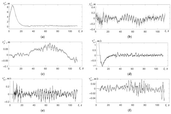
Figure 8.
The changing of the true and the predicted values of coordinates ((a) is the ; (b) is the ; (c) is the ) and speeds ((d) is the ; (e) is the ; (f) is the ) of target point in CS , taking into account the errors in determining the position and orientation of the AUV-leader.
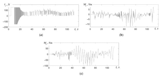
Figure 9.
The changes of control signals of AUV-follower, taking into account the errors in determining the position and orientation of the AUV-leader: (a) is the ; (b) is the ; (c) is the .
In general, the process of tracking the movements of the target point by the AUV-follower is stable and fairly accurate.
At the same time, the nature of this xF coordinate tracking is the same in both the first and second studies (see Figure 6a and Figure 8a, Figure 6b and Figure 8b, and Figure 7a and Figure 9a, respectively). However, it is a system in which the coordinates of the target point are determined precisely (see Figure 6); it works without jumps of errors and expectedly provides more accurate tracking.
In particular, the presence of errors in the information about the position and orientation of the AUV-leader leads to a deviation of the follower from its desired position up to 0.5 m at the xF coordinate, 0.25 m at the yF coordinate, and 0.2 m at the zF coordinate. This is explained by the appearance of sufficiently large errors in the operation of Expressions (7)–(11) for calculating the position of the target point (these errors can reach 0.3 m) because of errors in the array Ω, which lead to a less accurate approximation of the movement of the target point. However, despite the presence of such errors, Expressions (18), (22)–(25) allow the calculation of the speed of movement of the target point accurately and without delay and the prediction of its movement.
The errors value is greater the lower the frequency of the updating of the data received from the video camera and the greater the speed of AUV-leader because in the time interval between data updates the AUV-follower moves in accordance with the prediction that is being formed based on the inaccurate data from the onboard video camera. However, the presence of these errors still makes it possible to ensure the operability of the control system (29), (30) and (34) and the movement of the AUV-follower with dynamic accuracy sufficient to perform all types of underwater operations. Even if errors in the appropriate control channels increase sharply, then they are quickly worked out by the control system.
Figure 9 shows the control signals generated by the control system in the second study in the presence of errors in the estimates of the position of the target point.
It should be noted that in comparison with the results of work in [23], the proposed approach allows for sufficiently accurate movement of the AUV-follower in the case of the spatial movement of the group, as well as with speeds of more than 1.4 times and twice the data update period from the onboard video camera. At the same time, the system [23] loses its operability under these conditions.
Thus, the simulation results confirmed the workability and effectiveness of the proposed new method of forming the AUV cooperative control using light beacons that can be placed not only on the AUV-leader, but also on those following. It allows the use of the AUV-followers with simple onboard equipment for forming a complex AUV group structure.
6. Discussion
The results obtained in this work allow the confirmation of the possibility of implementing AUV formation control based on information received from the on-board cameras of the AUV-followers. At the same time, due to the features of obtaining video information under water, the distances between the AUV in the group cannot exceed 5–15 m. Movement at such distances with a relatively high speed requires fast updating of information about the leader position, as well as the use of control systems that allow for accurate movement of the followers and rapid response to changes in its trajectory. The proposed approach makes it possible to comprehensively solve these problems: the proposed algorithm for predicting the movement of the target point provides fast updating of information about the movement of the leader regardless of the period of data receipt from the onboard video camera of the AUV-follower, and the control system provides high accuracy of the AUV-follower movement.
At the same time, it should be noted that there were a number of tasks that were not considered in this work and will be solved in the future.
- 1.
- The development of a strategy for the movement of the AUV-followers in the case of loss of visual contact with the leader, as well as methods to avoid this.
- 2.
- The development of group control systems with a large number of AUVs and the study of the stability of the movement of such groups.
- 3.
- The modification of the proposed system for the case of movement in an environment containing obstacles.
7. Conclusions
The paper proposes a new method for the synthesis of spatial motion control systems of the AUV-leader and a group of AUV-followers during their cooperative movement in desired formation. This system allows the provision of an accurate positioning of the followers relative to the leader using information received with a low frequency only from their onboard video cameras. In order to improve the accuracy of the created system, it proposed the method of the estimation of the parameters of the movement of the AUV-leader (its speeds and accelerations) to predict its movement relative to the AUV-follower in the time intervals between updates of information received from the video cameras.
The main advantage of the proposed approach is the implementation of group movement in the leader–followers mode without the use of slow data exchange between them via acoustic communication channels, as well as without the use in the AUV-followers of expensive hydroacoustic navigation systems.
With the help of the proposed method, it is possible to organize the movement of large groups of AUV, when followers can act as leaders for one or more followers walking from the front or from the side.
This makes it possible to remove restrictions on the transparency of the underwater environment for the operation of AUV onboard video cameras, on the number of followers being moved, and on their location in the group.
Author Contributions
Conceptualization, V.F. and D.Y.; methodology, V.F. and D.Y.; software, D.Y.; formal analysis, D.Y.; investigation, D.Y.; resources, V.F. and D.Y.; data curation, D.Y.; writing—original draft preparation, D.Y.; writing—review and editing, V.F.; visualization, D.Y.; supervision, V.F.; project administration, V.F.; funding acquisition, V.F. All authors have read and agreed to the published version of the manuscript.
Funding
This research was funded by the Russian Science Foundation (grant 22-19-00392).
Institutional Review Board Statement
Not applicable.
Informed Consent Statement
Not applicable.
Data Availability Statement
There is no dataset associated with the paper.
Conflicts of Interest
The authors declare no conflict of interest.
References
- Das, B.; Subudhi, B.; Pati, B.B. Cooperative formation control of autonomous underwater vehicles: An overview. Int. J. Autom. Comput. 2016, 13, 199–225. [Google Scholar] [CrossRef]
- Besseghieur, K.L.; Trębiński, R.; Kaczmarek, W.; Panasiuk, J. From trajectory tracking control to Leader–Follower formation control. Cybern. Syst. 2020, 51, 339–356. [Google Scholar] [CrossRef]
- Das, K.; Fierro, R.; Kumar, V.; Ostrowski, J.P.; Spletzer, J.; Taylor, C.J. A vision-based formation control framework. IEEE Trans. Robot. Autom. 2002, 18, 813–825. [Google Scholar] [CrossRef]
- Bazoula, A.; Maaref, H. Fuzzy separation bearing control for mobile robots formation. Proc. World Acad. Sci. Eng. Technol. 2007, 1, 1–7. [Google Scholar]
- Li, X.; Xiao, J.; Cai, Z. Backstepping Based Multiple Mobile Robots Formation Control. In Proceedings of the 2005 IEEE/RSJ International Conference on Intelligent Robots and Systems (IROS 2005), Edmonton, AB, Canada, 2–6 August 2005; pp. 887–892. [Google Scholar]
- Subudhi, B.; Mohan, R.; Filaretov, V.; Zuev, A. Design of A Consensus Based Flocking Control Of Multiple Autonomous Underwater Vehicles Using Sliding Mode Approach. In Proceedings of the 28th DAAAM International Symposium, Zadar, Croatia, 8–11 November 2017; pp. 4–13. [Google Scholar]
- Maki, T.; Matsuda, T.; Sakamaki, T.; Ura, T.; Kojima, J. Navigation Method for Underwater Vehicles Based on Mutual Acoustical Positioning with a Single Seafloor Station. IEEE J. Ocean. Eng. 2013, 38, 167–177. [Google Scholar] [CrossRef]
- Atwood, D.; Leonard, J.; Bellingham, J.; Moran, B. An Acoustic Navigation System for Multiple Vehicles. In Proceedings of the International Symposium on Unmanned Untethered Submersible Technology, Durham, NH, USA, 25–27 September 1995; pp. 202–208. [Google Scholar]
- Filaretov, V.; Yukhimets, D. The method of path planning for AUV-group moving in desired formation in unknown environment with obstacles. IFAC-PapersOnLine 2020, 53, 14650–14655. [Google Scholar] [CrossRef]
- Caiti, A.; Calabrò, V.; Fabbri, T.; Fenucci, D.; Munafò, A. Underwater communication and distributed localization of AUV teams. In Proceedings of the MTS/IEEE International Conference OCEANS, Bergen, Norway, 10–13 June 2013; pp. 1–8. [Google Scholar]
- Rout, R.; Subudhi, B. A backstepping approach for the formation control of multiple autonomous underwater vehicles using a leader–follower strategy. J. Mar. Eng. Technol. 2016, 15, 38–46. [Google Scholar] [CrossRef]
- Eustice, R.; Whitcomb, L.; Singh, H.; Grund, M. Experimental Results in Synchronous-Clock One-Way-Travel-Time Acoustic Navigation for Autonomous Underwater Vehicles. In Proceedings of the 2007 IEEE International Conference on Robotics and Automation, Roma, Italy, 10–14 April 2007; pp. 4257–4264. [Google Scholar]
- Cario, G.; Casavola, A.; Djapic, V.; Gjanci, P.; Lupia, M.; Petrioli, C.; Spaccini, D. Clock Synchronization and Ranging Estimation for Control and Cooperation of Multiple UUVs. In Proceedings of the MTS/IEEE International Conference OCEANS, Shanghai, China, 10–13 April 2016. [Google Scholar]
- Filaretov, V.; Subudhi, B.; Yukhimets, D.; Mursalimov, E. The method of matching the navigation systems of AUV-leader and AUV-followers moving in formation. In Proceedings of the 2019 International Russian Automation Conference (RusAutoCon), Sochi, Russia, 8–14 September 2019. [Google Scholar]
- Zhao, Y.; Zhang, Y.; Lee, J. Lyapunov and sliding mode based leader-follower formation control for multiple mobile robots with an augmented distance-angle strategy. Int. J. Control. Autom. Syst. 2019, 17, 1314–1321. [Google Scholar] [CrossRef]
- Yan, Z.; Xu, D.; Chen, T.; Zhou, J. Formation control of unmanned underwater vehicles using local sensing means in absence of follower position information. Int. J. Adv. Robot. Syst. 2021, 18, 1–13. [Google Scholar] [CrossRef]
- Yazdani, A.; Sammut, K.; Yakimenko, O.; Lammas, A. A survey of underwater docking guidance systems. Robot. Auton. Syst. 2019, 124, 103382. [Google Scholar] [CrossRef]
- Indiveri, G. Geotechnical Surveys with Cooperative Autonomous Marine Vehicles: The EC WiMUST project. In Proceedings of the 2018 IEEE/OES Autonomous Underwater Vehicle Workshop (AUV), Porto, Portugal, 6–9 November 2018; pp. 1–6. [Google Scholar] [CrossRef]
- Streenan, A.; Du Toit, N. Diver relative AUV navigation for joint human-robot operations. In Proceedings of the 2013 OCEANS, San Diego, CA, USA, 23–27 September 2013; pp. 1–10. [Google Scholar] [CrossRef]
- Lwin, K.N.; Myint, M.; Mukada, N.; Yamada, D.; Matsuno, T.; Saitou, K.; Godou, W.; Sakamoto, T.; Minami, M. Sea Docking by Dual-eye Pose Estimation with Optimized Genetic Algorithm Parameters. J. Intell. Robot. Syst. 2019, 96, 245–266. [Google Scholar] [CrossRef]
- Figueiredo, A.; Ferreira, B.; Matos, A. Vision-based localization and positioning of an AUV. In Proceedings of the OCEANS 2016, Shanghai, China, 10–13 April 2016. [Google Scholar]
- Xiao, H.; Chen, X. Robotic target following with slow and delayed visual feedback. Int. J. Intell. Robot. Appl. 2020, 4, 378–389. [Google Scholar] [CrossRef]
- Filaretov, V.; Yukhimets, D. Formation control of AUV on the base of visual tracking of AUV-leader. In Proceedings of the International Russian Automation Conference (RusAutoCon), Sochi, Russia, 6–12 September 2021. [Google Scholar]
- Bradski, G.; Kaehler, A. Learning OpenCV: Computer Vision with the OpenCV Library; O’Reilly: Sebastopol, CA, USA, 2008. [Google Scholar]
- Fossen, T. Handbook of Marine Craft Hydrodynamics and Motion Control; Jonh Willey & Sons: Chichester, UK, 2011. [Google Scholar]
- Strutz, T. Data Fitting and Uncertainty: A Practical Introduction to Weighted Least Squares and Beyond, 2nd ed; Springer: Berlin/Heidelberg, Germany, 2016. [Google Scholar]
- Martins, J.R.; Sturdza, P.; Alonso, J.J. The complex-step derivative approximation. ACM Trans. Math. Softw. 2003, 29, 245–262. [Google Scholar] [CrossRef]
- Ikonen, E.; Najim, K. Advanced Process Identification and Control; Marcel Dekker: New York, NY, USA, 2002. [Google Scholar]
- Filaretov, V.F.; Yukhimets, D.A. Two-Loop System with Reference Model for Control of Spatial Movement of Cargo Underwater Vehicle. Mekhatronika Avtom. Upravlenie 2021, 22, 134–144. [Google Scholar] [CrossRef]
Publisher’s Note: MDPI stays neutral with regard to jurisdictional claims in published maps and institutional affiliations. |
© 2022 by the authors. Licensee MDPI, Basel, Switzerland. This article is an open access article distributed under the terms and conditions of the Creative Commons Attribution (CC BY) license (https://creativecommons.org/licenses/by/4.0/).