AUV Formation Coordination Control Based on Transformed Topology under Time-Varying Delay and Communication Interruption

Abstract

Aiming at the control problem of autonomous underwater vehicle (AUV) pilot-following formation with communication delay and communication interruption, a controller based on feedback linearization and the PD control method is designed in this paper. Firstly, the nonlinear, strongly coupled vehicle model is transformed into a second-order model via the feedback linearization method, and then the formation coordination controller is designed based on consistency theory and the PD control method. The Markov random jump process is used to simulate the formation topology in the event of communication interruption. The condition of stable convergence of the AUV pilot-following formation is analyzed in the presence of time-varying delay and Markov transformation topology. A Lyapunov–Krasovskii equation is established, and linear matrix inequality (LMI) is used to solve the problem of communication interruption and communication delay. The boundary conditions of error convergence of the control system are obtained. Finally, the effectiveness of the formation coordination controller based on the second-order integral model under the unstable conditions of underwater acoustic communication is verified by simulation.

1. Introduction

With the advancement of science and technology in the past few decades, considerable progress has been made in the field of autonomous underwater vehicles (AUVs) at home and abroad, and positive results have been achieved in various marine activities. AUV formation coordination control under limited communication has always been a research hotspot. It can be considered that each AUV in the formation must determine its position through its own equipment, and receive the current position and speed data of other AUVs through the acoustic communication channel [1]. However, the acoustic communication channel used for data exchange between underwater robots has the characteristics of prolonged transmission and communication interruption, and often cannot provide stable communication between AUV formation members. In order to eliminate the perturbation problem caused by the specific defects of the underwater acoustic communication channel, different authors have proposed different solutions.

The first important issue of the limitation of underwater communication is communication delay, which results in the followers in receiving inaccurate position and speed information on the leader and other neighbors for formation control. There are many similarities between AUVs and other multi-agent systems in communication, and numerous multi-agent studies on communication delay have been proposed. In order to reduce the effect of limited bandwidth in control, Rout et al. [2] proposed using an extended Kalman filter to design a controller for predicting the position of the leader AUV in the presence of communication skew, but if the initial state is not selected properly, it will cause the filter to diverge. Krstic [3] proposed a method based on predictor feedback for the time-varying sensor delay; however, this method is too computationally intensive, and is not suitable for practical systems. Yang et al. [4] studied the lead-following consistency problem for multi-agent systems with input delays, where the controller has too many control parameters, and it is difficult to adjust the parameters in practical applications. Araújo et al. [5] proposed a method for active vibration control to a two-link flexible robot arm in the presence of time delay, by means of robust pole placement. Singh et al. [6] presented a method for assigning complex poles to second-order damped asymmetric systems by using state-feedback control while considering a constant time delay in the feedback control loop. In [5,6], only the case of fixed delay instead of time-varying delay was studied. The stability of a closed-loop system was analyzed by computing primary closed-loop poles and the associated critical time delay. Han et al. [7] researched trajectory tracking of an underwater vehicle-manipulator system (UVMS) subjected to model uncertainties, time-varying external disturbances, payload, and sensory noises by combining an extended Kalman filter with inertial delay control. The downside of this article is that the establishment of fuzzy tables relies too much on experience, and the control system is too complicated and has poor portability.

Another important limitation of underwater communication is communication interruption; under this situation, the topology of the formation changes during the communication process. At present, many researchers have studied the consistency of systems based on switching topology. Reza et al. [8] studied the agent formation consistency problem with fixed and exchange topologies, but only the case of fixed delay instead of time-varying delay was studied. Ali et al. [9] designed a sampled data controller for the stability of a nonlinear multi-agent control system under directed switching topology, making the closed-loop system stable under uncertainty. Rahimi et al. [10] studied the design of a fault estimation controller for a class of nonlinear network systems with communication topology. In the solution, each agent utilizes an augmented system based on a given communication topology to estimate faults and states, including itself and its neighbors, where information received from neighbors is time-delayed. Finally, the relevant conditions in the form of linear matrix inequalities are deduced, proving the stability of the system; however, many issues are still open for future research, such as considering uncertainties in the parameters of agents and the quantization effects. Adhikari et al. [11] proposed a dynamical model-based tool to approximate synchronous behavior in large networks of interconnected linear systems with exchange topology and linear coupling. Zhang et al. [12] designed a local fault estimation observer for the output estimation error of each agent for the distributed fault estimation problem of multi-agent systems with switched topologies. Then, by introducing global variables, a global fault observer was proposed using the mean dwell time technique. In [8,9,10,12], the actual kinematic and dynamic models of multiple agents are not considered—the authors propose only abstract concepts. Park et al. [13] carried out consensus analysis and control of multi-agent systems with time-varying delays and Markovian switching interconnection topology via construction of a suitable Lyapunov–Krasovskii functional and utilization of a reciprocally convex approach. However, its dynamic performance needed to be improved, and multi-agent modeling was not carried out.

The above studies either only consider the communication time delay or only consider the communication interruption, and so they do not conform to the actual situation of unstable communication in the underwater acoustic channel. Most of them only consider cases in a two-dimensional environment. Based on the above analysis, it can be seen that there are still many difficulties in the accurate 3D trajectory control of AUVs in the context of communication interruption and communication delay.

The original contribution of this paper is that the accurate feedback linearization model is used for the actuated AUV, the nonlinear model is linearized by the method of feedback linearization, and the complex model is transformed into a linear second-order integral model, The output of the controller under this model is converted into the actual thrust and torque through the coordinate conversion formula to control the AUV. This is a brand new method to convert an AUV’s actual nonlinear model to a simple linear model, which effectively simplifies the process of designing the controller and eliminates the systematic error of the nonlinear model. Furthermore, in this paper, a formation controller is designed, and the control gain range for maintaining the formation is given by solving the LMI, which provides a theoretical basis for the establishment of parameters and proof of stability, and finally achieves the accurate 3D trajectory control of the AUV in the circumstances of both communication interruption and communication delay, and verifies its performance. Compared with the controllers in the above papers, our controller is easy to design, has strong portability, and has better dynamic performance. The upper and lower bounds of the parameters are proven theoretically, which reduces the manpower and time required for parameter adjustment, and is better for practical applications.

2. Construction of the AUV Feedback Linearization Model

The AUV coordinate diagram is shown in Figure 1, where $E - \xi \eta \zeta$ is the geodetic coordinate system, $\xi$ points due north, $\eta$ points due east, $O-xyz$ is the hull coordinate system, and $O$ coincides with the center of gravity of the AUV, where the x-axis points to the bow of the vehicle. To facilitate subsequent research, the following variables are defined:

The location of the geodetic coordinate system is ${\eta }_1={[xyz]}^T\in R^3$.

The attitude angle is ${\eta }_2={[\phi \theta \psi ]}^T\in S^3$.

The linear velocity of the hull coordinate system is ${\nu }_1={[uvw]}^T\in R^3$.

The angular velocity is ${\nu }_2={[pqr]}^T\in R^3$.

The thrust is ${\tau }_1={[{\tau }_u{\tau }_v{\tau }_w]}^T\in R^3$.

The torque is ${\tau }_2={[{\tau }_p{\tau }_q{\tau }_r]}^T\in R^3$.

Where $R^3$ represents the three-dimensional Euclidean space and $S^3$ represents the three-dimensional torus. The AUV selected in this paper can be approximately regarded as a micro-flat shape with up and down symmetry, left and right symmetry, and large heel damping. In practical engineering, the rolling motion is usually self-stabilizing, and the rolling amplitude is small, which can be approximately regarded as 0 for the heel angle and 0 for the heel angular velocity.

The actuators of the AUV can be described as follows: the main thrusters of the AUV are arranged at the stern of the vehicle, and are responsible for the motion control of the AUV in the x-direction; the auxiliary thrusters of the AUV are arranged on both sides and at the top of the vehicle, and are responsible for the y-direction and z-direction of the AUV’s motion control; the vertical rudder of the AUV is responsible for the steering motion control of the aircraft; the horizontal rudder of the AUV is responsible for the trim motion control of the vehicle. The three-dimensional space motion of the AUV has characteristics of actuating, and its mathematical model is established in the hull coordinate system as follows:

$$\{\begin{array}{l}\dot{\eta }=J(\eta )v\\ M\dot{v}=g^{\prime }\tau -C(v)v-D(v)v-g(\eta )\end{array}$$

(1)

where $\eta ={(x,y,z,\theta ,\psi )}^T\in R^5$ represents the position and attitude vector of the AUV in a fixed coordinate system, and the velocity variables of the AUV in each direction in the hull coordinate system are as follows: $v={(u,v,w,q,r)}^T\in R^5$ shows the position and attitude vector of the AUV in a fixed coordinate system; $M$ is the inertia matrix; $J(\eta )$ is the transformation matrix; $C(v)$ is the Coriolis force and centripetal force matrix; $D(v)$ is the lift moment and hydrodynamic matrix; $g(\eta )$ represents the restoring force and moment vectors; $\tau ={({\tau }_u,{\tau }_v,{\tau }_w,{\tau }_q,{\tau }_r)}^T\in R^5$ is the control input of the AUV’s actuator; and $g^{\prime }\in R^{5\times 5}$ is the actuator parameter matrix.

The kinematic and dynamic mathematical models and model parameters of the AUV are shown in [14].

First, the relevant knowledge of the model feedback linearization method is introduced [15] as follows:

Definition 1.

[Vector field] Take a nonlinear first-order model:

$$\begin{array}{l}\dot{x}=f(x)+g(x)u\\ y=h(x)\end{array}$$

(2)

In (2), if $f(x),g(x),h(x)$ is smooth enough in the definition domain $D\in R^n$, then the mapping $f:D\to R^n$ and $g:D\to R^n$ represents the vector fields of definition domain $D$.

Definition 2.

[Lie derivative] Differentiate y in(2):

$$\dot{y}=\frac{\partial h}{\partial x}[f(x)+g(x)u]=L_{f}h(x)+L_{g}h(x)u$$

(3)

where$L_{f}h(x)=\frac{\partial h}{\partial x}f(x)$,$L_{g}h(x)=\frac{\partial h}{\partial x}g(x)$,and$h:D\to R^n$is called the Lie derivative of the smooth vector field$f$.

In the related theory of differential geometry, the Lie derivative contains an important property: if $h(x)$ is a smooth function, then $L_{f}h(x)$ is also a smooth function. Thus, the second derivative of y is:

$$\ddot{y}=\frac{\partial (L_{f}h(x))}{\partial x}[f(x)+g(x)u]$$

(4)

Definition 3.

[Relative order] If there is an$\rho$-order derivative of $y$,

$$y^{\rho }=\frac{\partial (L_f^{\rho -1}h(x))}{\partial x}[f(x)+g(x)u]=L_f^{\rho }h(x)+L_g{L}_f^{\rho -1}h(x)u$$

(5)

If$L_g{L}_f^{\rho -1}h(x)\ne 0$, and$0\le r\le \rho -2$,$L_g{L}_f^{r}h(x)=0$, then the nonlinear control system—that is, (2)—has a relative order$\rho$in its definition domain$x\in D$.

Definition 4.

[MIMO relative order] If there is the following multi-order nonlinear system

$$\begin{array}{l}\dot{x}=f(x)+g(x)u\\ y=h(x)\end{array}$$

(6)

where$x$is a n-dimensional state variable,$y$is a m-dimensional state variable,$f(x)$and$g_i(x)$are the dimensional vector fields, and $g(x)=[g_1(x),g_2(x),\dots ,g_m(x)]$,$h(x)={[h_1(x),h_2(x),\dots ,h_m(x)]}^T$,$u={[u_1,u_2,\dots ,u_n]}^T$are the control inputs to the model.

$$L_{gj}{L}_f^{{\rho }_i-1}{h}_i(x)=0\hspace{1em}\hspace{1em}\hspace{1em}i,j\in \{1,2,\dots ,m\}$$

(7)

Then, for any $1\le i\le m$, there is at least one $j$ satisfying $L_{gj}{L}_f^{{\rho }_i-1}{h}_i(x)\ne 0$, and there is an $m\times m$ dimensional matrix:

$$\Gamma (x)=\left[\begin{array}{ccc}{L}_{g1}{L}_f^{{\rho }_1-1}{h}_1(x)& \cdots & L_{gm}{L}_f^{{\rho }_1-1}{h}_i(x)\\ L_{g1}{L}_f^{\rho 2-1}{h}_1(x)& \cdots & L_{gm}{L}_f^{\rho 2-1}{h}_i(x)\\ ⋮& \ddots & \begin{array}{cc}& \end{array}⋮\\ L_{g1}{L}_f^{\rho m-1}{h}_1(x)& \cdots & L_{gm}{L}_f^{\rho m-1}{h}_i(x)\end{array}\right]$$

(8)

If $\Gamma (x)$ is a nonsingular matrix, then $\rho ={\displaystyle \sum _{i=1}^m{\rho }_i}$ is the relative order of the MIMO system, and ${\rho }_i$ is the relative order of each subsystem $h_i(x)$.

According to the relationship between the relative order $\rho$ and the order of the control system $n$, it can be divided into two cases: if $\rho =n$, then the exact feedback linearization of (6) can be performed, and if $\rho <n$, then part of (6) can be linearized.

According to the research object of this paper, the AUV model is appropriately transformed:

$$\{\begin{array}{l}\dot{\eta }=J(\eta )v\\ \dot{v}=M^{-1}{g}^{\prime }\tau +M^{-1}N(\eta ,v)\end{array}$$

(9)

In order to facilitate the linearization of the model, (9) is written in the following form:

$$\dot{\xi }=f(\xi )+M_1{g}^{\prime }\tau$$

(10)

If the output of the nonlinear system is the position and attitude state, then the nonlinear model of the AUV is:

$$\{\begin{array}{l}\dot{\xi }=f(\xi )+g(\xi )\tau \\ \varsigma =h(\xi )\end{array}$$

(11)

and $h(\xi )={(x,y,z,\theta ,\psi )}^T$, $g(\xi )=M_1{g}^{\prime }$.

According to the Lie derivative, it can be known that:

$$\dot{\varsigma }=\frac{\partial h}{\partial \xi }(f(\xi )+g(\xi ))$$

(12)

The first-order Lie derivative $L_{f}h(\xi )$, $L_{g}h(\xi )$ can be obtained, which has the following form:

$$\{\begin{array}{l}{L}_{f}h(\xi )=J(\eta )v\ne 0\\ L_{g}h(\xi )=0\end{array}$$

(13)

Similarly, according to the definition of the second-order Lie derivative, it can be known that:

$$\ddot{\varsigma }=\frac{\partial L_{f}h(\xi )}{\partial \xi }(f(\xi )+g(\xi )\tau )$$

(14)

and the second-order Lie derivative $L_f^{2}h(\xi )$, $L_g{L}_{f}h(\xi )$ has the following form:

$$\{\begin{array}{l}{L}_f^{2}h(\xi )=\frac{\partial L_{f}h(\xi )}{\partial \xi }f(\xi )\ne 0\\ L_g{L}_{f}h(\xi )=\frac{\partial L_{f}h(\xi )}{\partial \xi }g(\xi )\ne 0\end{array}$$

(15)

The relative order sum of this AUV model is ${\rho }_1+{\rho }_2+{\rho }_3+{\rho }_4+{\rho }_5=10$, and ${\rho }_1={\rho }_2={\rho }_3={\rho }_4={\rho }_5=2$; that is, the order of the relative order is equal to the order of the system: 10. Therefore, the feedback linearization method can be accurately applied to this AUV model and find a solution. The design coordinates change as follows:

$$\{\begin{array}{l}{z}_1(\xi )={(h_1(\xi ),h_2(\xi ),h_3(\xi ),h_4(\xi ),h_5(\xi ))}^T\\ z_2(\xi )={(L_f{h}_1(\xi ),L_f{h}_2(\xi ),L_f{h}_3(\xi ),L_f{h}_4(\xi ),L_f{h}_5(\xi ))}^T\end{array}$$

(16)

Substitute (13) into (16):

$$\{\begin{array}{l}{\dot{z}}_1=z_2\\ {\dot{z}}_2=L_f^{2}h(\xi )+L_g{L}_{f}h(\xi )\tau \end{array}$$

(17)

If $U=L_f^{2}h(\xi )+L_g{L}_{f}h(\xi )\tau$, then after coordinate transformation the control input of the actual nonlinear model can be obtained as $\tau ={(L_g{L}_{f}h(\xi ))}^{-1}(U-L_f^{2}h(\xi ))$. The mathematical model after AUV linearization is obtained as follows:

$$\{\begin{array}{l}{\dot{z}}_1=z_2\\ {\dot{z}}_2=U\end{array}$$

(18)

3. Control Law and Consensus Analysis

The exchange topology is represented by a directed graph, and the value of the elements $l_{ij}$ in the adjacency matrix $L=\left[l_{ij}\right]\in R^{N\times N}$ satisfies $l_{ij}\ge 0$. The element value in the adjacency matrix can be designed according to the task requirements; that is, the larger value $l_{ij}$ is designed for the edge $(i,j)$ with better connectivity, which can also improve the convergence speed when formations are formed. Assume that the formation time-varying communication delay names $\tau (t)$, which satisfies $0<\tau (t)<h_d$, and the derivative satisfies $\dot{\tau }(t)<r<1$. The following are the lemmas and definition of this section:

Definition 5.

[Kronecker product].

Given two matrices$A\in {ℝ}^{m\times n},B\in {ℝ}^{p\times q}$, if the matrix$H\in {ℝ}^{mp\times nq}$satisfies the following equation, then the matrix$H$is called the Kronecker product of the matrices$A$and $B$, which is written as$A\otimes B$.

$$H=A\otimes B=\left[\begin{array}{ccc}{a}_{11}B& \cdots & a_{1n}B\\ ⋮& \ddots & ⋮\\ a_{m1}B& \cdots & a_{mn}B\end{array}\right],A=\left[\begin{array}{ccc}{a}_{11}& \cdots & a_{1n}\\ ⋮& \ddots & ⋮\\ a_{m1}& \cdots & a_{mn}\end{array}\right]$$

(19)

Lemma 1

([16]).Assuming that$f(t)$is$F_t$measurable, where$F_t$is a filtration,and$t\in R^{+}$and$E\left[f(t)1_{\left(\theta =i\right)}\right]=f_i(t)$exist, for any$i\in n$, there are:

$$E\left[f(x)d(1_{\left(\theta =i\right)})\right]={\displaystyle \sum _{j=1}^n{\lambda }_{ji}E}\left[f(x)1_{\left(\theta =j\right)}\right]dt+o(dt)$$

(20)

where$\theta =\{({\theta }_t,F_t),t\in R^{+}\}$is a homogeneous Markov process taking values on the set t, and $[({\lambda }_{ij})]$ is the stationary infinite-dimensional transition rate matrix of $0\le {\lambda }_{ij},i\ne j$ and $0\le {\lambda }_i:=-{\lambda }_{ii}={\displaystyle {\sum }_{\left(j:j\ne i\right)}{\lambda }_{ij}\le \sigma }$ for all, where $\sigma$ is a constant.

Proof of Lemma 1.

Bearing in mind that $d(1_{\{{\theta }_t=i\}}):=1_{\{{\theta }_{t+dt}=i\}}-1_{\{{\theta }_t=i\}}$

, we have:

$$\begin{array}{ll}E\left[f(t)d(1_{\left(\theta =i\right)})\right]& =E(f(t)1_{\{{\theta }_{t+dt}=i\}})-E(f(t)1_{\{{\theta }_t=i\}})\\ & ={\displaystyle \sum _{j=1}^{\infty }E(E(f(t))}{1}_{\{{\theta }_{t+dt}=i\}}{1}_{\{{\theta }_t=j\}}|F_t)-E(f(t)1_{\{{\theta }_t=i\}})\\ & ={\displaystyle \sum _{j=1}^{\infty }\mathbb{P}({\theta }_{t+dt}=i|{\theta }_i=j)}{f}_j\left(t\right)-f_i(t)\\ & ={\displaystyle \sum _{j=1}^n{\lambda }_{ji}{f}_j}(t)dt+o(dt)\end{array}$$

(21)

□

Lemma 2 ([17]).

For the constant real matrix $M=M^T>0,M\in R^{N\times N}$, where$\tau >0,\left\{x(s)|t-\tau \le s\le t\right\}\to R^n$exists, the following formula is established:

$$-\tau {\displaystyle \int {}_{t-\tau }^t}{\dot{x}}^T(s)M\dot{x}(s)ds\le -{\left[x(t)-x(t-\tau )\right]}^{T}M\left[x(t)-x(t-\tau )\right]$$

(22)

Proof of Lemma 2:

We can easily get:

$${\left[x(t)-x(t-\tau )\right]}^{T}M\left[x(t)-x(t-\tau )\right]\le {({\displaystyle \int {}_{-\tau }^0}\dot{x}(t+\xi )d\xi )}^{T}M({\displaystyle \int {}_{-\tau }^0}\dot{x}(t+\xi )d\xi )$$

(23)

and then use Lemma 1 in [18] to obtain:

$$\tau {\displaystyle \int {}_{-\tau }^0}{\dot{x}}^T(t+\xi )M\dot{x}(t+\xi )d\xi \ge {({\displaystyle \int {}_{-\tau }^0}\dot{x}(t+\xi )d\xi )}^{T}M({\displaystyle \int {}_{-\tau }^0}\dot{x}(t+\xi )d\xi )$$

(24)

□

Using Schur’s complement that:

$$\left(\begin{array}{cc}{x}^T(\xi )Mx(\xi )& x^T(\xi )\\ x(\xi )& M^{-1}\end{array}\right)\ge 0$$

(25)

for any $0\le \xi \le \tau$. Integration of the above inequality from 0 to $\tau$ yields:

$$\left(\begin{array}{cc}{\displaystyle {\int }_0^{\tau }{x}^T(\xi )Mx(\xi )d\xi }& {\displaystyle {\int }_0^{\tau }{x}^T(\xi )d\xi }\\ {\displaystyle {\int }_0^{\tau }x(\xi )d\xi }& \tau M^{-1}\end{array}\right)\ge 0$$

(26)

In this way, (24) is proven, and then so is (23).

If we define the acceleration of the ith follower as ${\dot{v}}_i(t)$, then the control input of the second-order integral model after the linear feedback of the ith follower AUV is:

$$\begin{array}{ll}{u}_{ni}(t)=& -\alpha {\displaystyle \sum _{j=1}^N{a}_{ij}(t)({\sigma }_i(t-\tau (t))-{\sigma }_j(t-\tau (t)))-\beta {\displaystyle \sum _{j=1}^N{a}_{ij}(t)(v_i(t-\tau (t))-v_j(t-\tau (t)))}}\\ & -\alpha c_{il}(t)({\sigma }_i(t-\tau (t))-{\sigma }_l(t-\tau (t)))-\beta c_{il}(t)(v_i(t-\tau (t))-v_l(t-\tau (t)))\\ & -\gamma {\displaystyle \sum _{j=1}^N{a}_{ij}(t)({\dot{v}}_i(t-\tau (t))-{\dot{v}}_j(t-\tau (t)))}\end{array}$$

(27)

where ${\sigma }_i(t)$ represents the position state of the ith AUV, $\alpha$ represents the position gain, $\beta$ represents the velocity gain, $a_{ij}(t)$ is the (i,j)th unit of the adjacency matrix of the communication between the followers, ${\sigma }_l(t)$ is the position state and $v_l(t)$ is the speed state of the leader in the formation, $c_{il}(t)$ represents the communication relationship between the ith follower AUV and the leader AUV, $\gamma$ is the acceleration gain, and $\tau (t)$ is the time-varying delay, which changes with time.

Define $\mu (t)={[{\sigma }_1^T(t){\sigma }_2^T(t)\dots {\sigma }_n^T(t)]}^T$ as the position and attitude state of the AUV formation, $\xi (t)={[v_1^T(t)v_2^T(t)\dots v_n^T(t)]}^T$ as the speed state of the AUV formation, $L_1$ as the Laplacian matrix of the follower AUV communication topology, and $L_2$ as the communication state matrix of the leader and the follower. Define the system state error of the AUV formation as $E(t)={[E_x^T(t)E_v^T(t)]}^T$, where $E_x(t)=\mu (t)-1_n{\sigma }_l(t)$, $E_v(t)=\xi (t)-1_n{v}_l(t)$, $1_n$ represent an n-dimensional column vector whose elements are all 1. The state equation of the error can be obtained from (27) as follows:

$$\dot{E}(t)=AE(t)+BE(t-\tau (t))+C\dot{E}(t-\tau (t))$$

(28)

where matrix $A=\left[\begin{array}{cc}0& I\\ 0& 0\end{array}\right]\otimes I_5$, matrix $B=\left[\begin{array}{cc}0& 0\\ -\alpha (L_1(t)+L_2(t))& -\beta (L_1(t)+L_2(t))\end{array}\right]\otimes I_5$, and matrix $C=\left[\begin{array}{cc}0& 0\\ 0& -\gamma L_1(t)\end{array}\right]\otimes I_5$.

Theorem 1.

If there are real symmetric matrices$P\ge 0,Q\ge 0,R\ge 0$, the directed topology graph contains spanning trees, the value of the elements$l_{ij}$in the adjacency matrix$L=\left[l_{ij}\right]\in R^{N\times N}$satisfies $l_{ij}\ge 0$, the formation’s time-varying communication delay$\tau (t)$satisfies$0<\tau (t)<h_d$and the derivative satisfies$\dot{\tau }(t)<r<1$, and the followingLMI holds, then the AUV formation based on feedback linearization under the time-varying delay $\tau (t)$ and transformation topology can form the desiredformation and keepitselfstable.

$$\left[\begin{array}{cccc}{\psi }_{11}& {\psi }_{12}& 0& PC+2h_d{A}^{T}RC\\ \ast & 2h_d{B}^{T}RB-2h_d{}^{-1}R& h_d{}^{-1}R& 2h_d{B}^{T}RC\\ \ast & \ast & (r-1)Q-h_d{}^{-1}R& 0\\ \ast & \ast & \ast & 2h_d{C}^{T}RC\end{array}\right]<0$$

(29)

where${\psi }_{11}=A^{T}P+PA+Q+2h_d{A}^{T}RA-h_d{}^{-1}R$, ${\psi }_{12}=PB+h_d{}^{-1}R+2h_d{A}^{T}RB$.

Assuming that the upper bound of the delay $h_d$ and the communication topology matrix $L_1,L_2$ are already known, the equation can be solved using the LMI toolbox in MATLAB to obtain the range of control gains $\alpha ,\beta ,\gamma$.

Proof of Theorem 1.

For the formation communication topology set with number n, the following Lyapunov–Krasovskii expectation equation is constructed for the kth topology:

$$\begin{array}{ll}{V}^k(t)=& E\left(E^T(t)PE(t)1_{\left\{\theta (t)=k\right\}}\right)\\ & +E\left({\displaystyle {\int }_{t-\tau }^t{E}^T(s)QE(s)}ds{1}_{\left\{\theta (t)=k\right\}}+{\displaystyle {\int }_{t-h_d-\tau }^{t-\tau }{E}^T(s)QE(s)}ds{1}_{\left\{\theta (t)=k\right\}}\right)\\ & +E\left({\displaystyle {\int }_{-h_d}^0{\displaystyle {\int }_{t+\theta }^t{\dot{E}}^T(s)R\dot{E}(s)}}dsd\theta 1_{\left\{\theta (t)=k\right\}}+{\displaystyle {\int }_{-h_d-\tau }^{-\tau }{\displaystyle {\int }_{t+\theta }^t{\dot{E}}^T(s)R\dot{E}(s)}}dsd\theta 1_{\left\{\theta (t)=k\right\}}\right)\end{array}$$

(30)

□

The above formula can be constructed into three sub-functions, and their derivation can be obtained:

$$d\left(V_1^k(t)1_{\left\{\theta (t)=k\right\}}\right)=d{E}^T(t)PE(t)1_{\left\{\theta (t)=k\right\}}+E^T(t)PdE(t)1_{\left\{\theta (t)=k\right\}}+E^T(t)PE(t)d{1}_{\left\{\theta (t)=k\right\}}$$

(31)

$$\begin{array}{ll}d\left(V_2^k(t)1_{\left\{\theta (t)=k\right\}}\right)& =d\left({\displaystyle {\int }_{t-\tau }^t{E}^T(s)QE(s)}ds+{\displaystyle {\int }_{t-h_d-\tau }^{t-\tau }{E}^T(s)QE(s)}ds\right)1_{\left\{\theta (t)=k\right\}}\\ & +\left({\displaystyle {\int }_{t-\tau }^t{E}^T(s)QE(s)}ds+{\displaystyle {\int }_{t-h_d-\tau }^{t-\tau }{E}^T(s)QE(s)}ds\right)d{1}_{\left\{\theta (t)=k\right\}}\end{array}$$

(32)

$$\begin{array}{ll}d\left(V_3^k(t)1_{\left\{\theta (t)=k\right\}}\right)& =d\left({\displaystyle {\int }_{-h_d}^0{\displaystyle {\int }_{t+\theta }^t{\dot{E}}^T(s)R\dot{E}(s)}}dsd\theta +{\displaystyle {\int }_{-h_d-\tau }^{-\tau }{\displaystyle {\int }_{t+\theta }^t{\dot{E}}^T(s)R\dot{E}(s)}}dsd\theta \right)1_{\left\{\theta (t)=k\right\}}\\ & +\left({\displaystyle {\int }_{-h_d}^0{\displaystyle {\int }_{t+\theta }^t{\dot{E}}^T(s)R\dot{E}(s)}}dsd\theta +{\displaystyle {\int }_{-h_d-\tau }^{-\tau }{\displaystyle {\int }_{t+\theta }^t{\dot{E}}^T(s)R\dot{E}(s)}}dsd\theta \right)d{1}_{\left\{\theta (t)=k\right\}}\end{array}$$

(33)

If we replace $\tau (t)$ with ${\tau }_1$, $\tau (t)+h_d$ with ${\tau }_2$, and refer to Lemmas 1 and 2, the derivative of the topological Lyapunov equation can be expressed as follows:

$$\begin{array}{ll}d\left({\overline{V}}^k(t)\right)& \le E\{{\dot{E}}^T(t)PE(t)1_{\left\{\theta (t)=k\right\}}+E^T(t)P\dot{E}(t)1_{\left\{\theta (t)=k\right\}}+E^T(t)QE(t)1_{\left\{\theta (t)=k\right\}}\\ & -(1-r)E^T(t-{\tau }_2)QE(t-{\tau }_2)1_{\left\{\theta (t)=k\right\}}+2h_d{\dot{E}}^T(t)R\dot{E}(t)1_{\left\{\theta (t)=k\right\}}\\ & -h_d^{-1}{[E(t-{\tau }_1)-E(t-{\tau }_2)]}^{T}R[E(t-{\tau }_1)-E(t-{\tau }_2)]1_{\left\{\theta (t)=k\right\}}\\ & -h_d^{-1}{[E(t)-E(t-{\tau }_1)]}^{T}R[E(t)-E(t-{\tau }_1)]1_{\{\theta (t)=k\}}\}+{\displaystyle \sum _{j=1}^N{\lambda }_{ji}{\overline{V}}^j(t)dt}\end{array}$$

(34)

Taking into account joint communication topologies:

$$\overline{V}={\displaystyle \sum _{i=1}^N{V}^i(\cdot )}$$

(35)

and according to the Markov stochastic process, we can get:

$${\displaystyle \sum _{i=1}^N{\lambda }_{ji}=0}$$

(36)

Thus, ${\displaystyle \sum _{j=1}^N{\lambda }_{ji}{\overline{V}}^j(t)dt=0}$.

If we substitute (28) into (34) and define the matrix $\overline{A}=A\otimes I_n,\overline{B}=B\otimes I_n,\overline{C}=C\otimes I_n$, the derivative of the Lyapunov equation $\dot{V}(t)$ of the communication topology set can be obtained as follows:

$$\begin{array}{ll}\dot{V}(t)& \le E\{E^T(t)\left(A^{T}P+PA+Q\right)E(t)+E^T(t-{\tau }_1)B^{T}PE(t)+{\dot{E}}^T(t-{\tau }_1)C^{T}PE(t)\\ & +E^T(t)PBE(t-{\tau }_1)+E^T(t)PC\dot{E}(t-{\tau }_1)+(1-r)E^T(t-{\tau }_2)QE(t-{\tau }_2)\\ & +2h_d[E^T(t)A^{T}RAE(t)+E^T(t)A^{T}RBE(t-{\tau }_1)+E^T(t)A^{T}RC\dot{E}(t-{\tau }_1)\\ & E^T(t-{\tau }_1)B^{T}RAE(t)+E^T(t-{\tau }_1)B^{T}RBE(t-{\tau }_1)+E^T(t-{\tau }_1)B^{T}RC\dot{E}(t-{\tau }_1)\\ & {\dot{E}}^T(t-{\tau }_1)C^{T}RAE(t)+{\dot{E}}^T(t-{\tau }_1)C^{T}RBE(t-{\tau }_1)+{\dot{E}}^T(t-{\tau }_1)C^{T}RC\dot{E}(t-{\tau }_1)]\\ & -h_d^{-1}{[E(t-{\tau }_1)-E(t-{\tau }_2)]}^{T}R[E(t-{\tau }_1)-E(t-{\tau }_2)]\\ & -h_d^{-1}{[E(t)-E(t-{\tau }_1)]}^{T}R[E(t)-E(t-{\tau }_1)]\}\end{array}$$

(37)

Let the vector $\varsigma (t)={[E^T(t),E^T(t-{\tau }_1),E^T(t-{\tau }_2),{\dot{E}}^T(t-{\tau }_1)]}^T$, and define the matrix $e_i\in R^{nN\times 4nN}$; if i = 1, then $e_1=[I_{nN}000]$, and (34) can be written as follows:

$$\dot{V}(t)\le E\{{\varsigma }^T(t)S\varsigma (t)\}$$

(38)

where the matrix $S$ is defined as follows:

$$\begin{array}{ll}S=& e_1^T(t)[A^{T}P+PA+Q+2h_d{A}^{T}RA-h_d{}^{-1}R]e_1(t)+e_1^T(t)[PB+h_d{}^{-1}R+2h_d{A}^{T}RB]e_2(t)\\ & +e_1^T(t)[PC+2h_d{A}^{T}RC]e_4(t)+e_2^T(t)[B^{T}P+h_d{}^{-1}R+2h_d{B}^{T}RA]e_1(t)+e_2^T(t)[h_d{}^{-1}R]e_3(t)\\ & +e_2^T(t)[2h_d{B}^{T}RB-2h_d{}^{-1}R]e_2(t)+e_2^T(t)[2h_d{B}^{T}RC]e_4(t)+e_3^T(t)[h_d{}^{-1}R]e_2(t)\\ & +e_3^T(t)[(r-1)Q-h_d{}^{-1}R]e_3(t)+e_4^T(t)[C^{T}P+2h_d{C}^{T}RA]e_1(t)\\ & +e_4^T(t)[2h_d{C}^{T}RB]e_2(t)+e_4^T(t)[2h_d{C}^{T}RC]e_4(t)\end{array}$$

(39)

The matrix $S<0$ when LMI in (29) holds; thus, the derivative of the error of the AUV formation under the communication topology set $\dot{V}(t) < 0$ in (38). Under the above conditions, it can be concluded that the formation can ensure stable convergence through PD control under the presence of Markov switching topology and time-varying delay.

4. Simulation Results

The AUV of the simulation experiment in this paper was selected from the simulation experiment object in [14]. The main model parameters are as follows in

Table 1. The main parameters of AUV model.

Parameter	Value	Unit
M	5783.1	Kg
L	5	M
ρ	1025	Kg/m3
Maximum thrust	1000	N
Maximum rudder	35	Deg
Maximum speed	6	Kn

:

The detailed model parameters of AUV can be found in [14].

Firstly, the PD control with Markov switching topology and time-varying delay is simulated, considering the AUV formation with one leader and four followers, and the adjacency matrix value $l_{ij}$ in the topology is not unique. The leader is represented by the number 0, and the remaining four followers are marked by the numbers 1–4. The Laplacian matrices $L_1(t)$ and $L_2(t)$ are represented by a topology diagram. The specific structure is as follows:

In Figure 2, the dotted lines represent the directional communication relationship between the followers and the leader in the formation, while the solid lines represent the directional communication relationships between each follower in the formation. $G_1,G_2,G_3,G_4$ are the four communication topologies in the topology set; thus, the number of topology sets $n=4$, G represents the joint topology generated by the topology set, and it can be seen from the figure that G contains a spanning tree. In the simulation, the first 800 s topologies are constantly switched in the topology set, and the topology is G, which is a fixed topology from 800 s to 1000 s.

By increasing the upper bound of delay $h_d$ every 0.01 s from 0 in the LMI toolbox, the maximum delay that the system can solve for the control gain is 2.09 s. Defining the time-varying delay variable $\tau (t)=0.8\sin (t)$, the obtained ranges of control gains are $\alpha < 0.24,\beta < 1.87,\gamma < 0.39$.

The initial position of each follower AUV is randomly distributed from 0 to 60 m in the x direction, 0 to 50 m in the y direction, and 0 to −10 m in the z direction, and the initial longitudinal velocity is 0 to 0.5 m/s. The control gains are $\alpha =0.0273,\beta =0.8375,\gamma =0.0848$. The expected deviations of the four followers from the leader in the x direction are: −10 m, 10 m, −20 m, and 20 m, respectively, and the movement trajectory of the leader is as follows:

$$\{\begin{array}{l}{x}_l=60\cos (0.002\pi t)\\ y_l=60\sin (0.002\pi t)\\ z_l=-0.03t\end{array}0\le t\le 1000$$

(40)

The change in topology in the first 800 s during the simulation process is shown in Figure 3. The states of the remaining formations include the position and attitude state, speed state, and acceleration state. The structure is as follows:

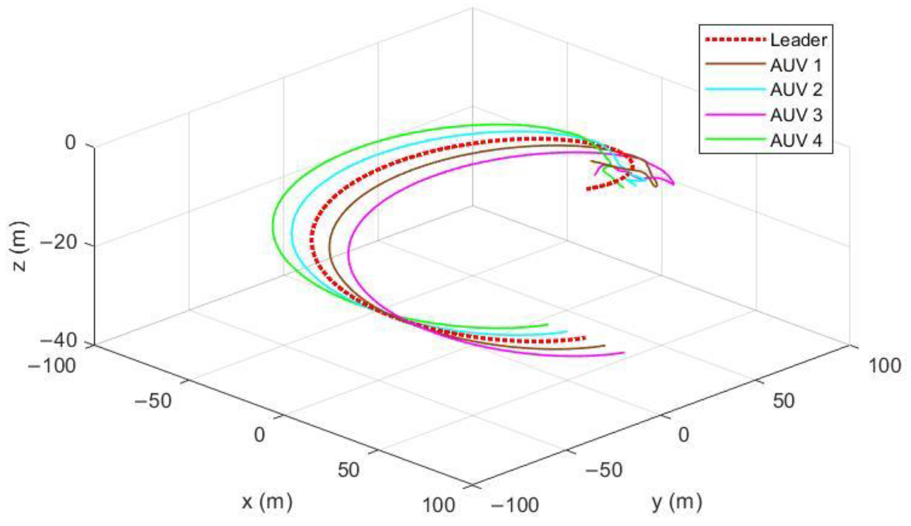
Figure 4 and Figure 5 show the three-dimensional and two-dimensional tracks of the AUV formation, respectively. It can be seen that the tracks of the AUV formation have gradually changed from the disorder at the beginning to a regular spiral dive formation, and maintained a distance of 10 m from one another. Videos S1 and S2 in supplementary materials demonstrate this process.

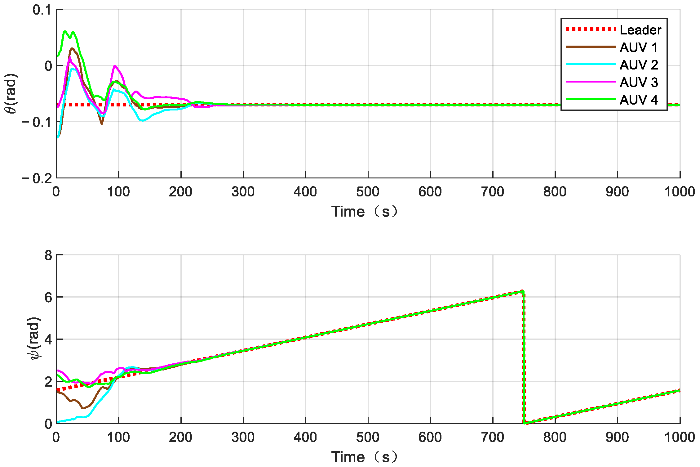
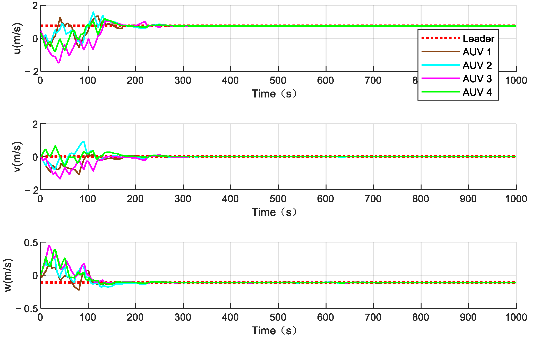
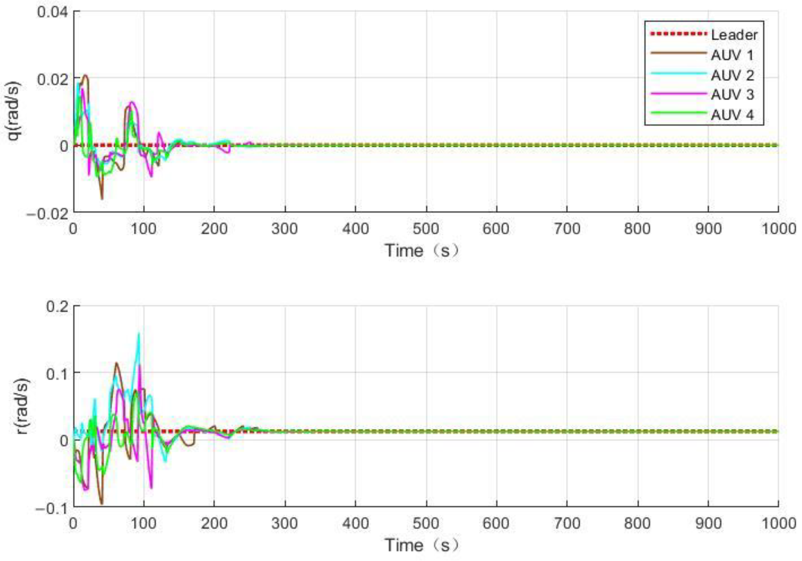
Figure 6, Figure 7, Figure 8 and Figure 9 show the position and speed of the AUV formation. It can be seen that the formation can stably converge in about 200 s and track the desired path at a speed of 1.5 m/s. Although the speed fluctuates in the initial state, the fluctuation range does not exceed 1 m/s, and the frequency is between 10 and 20 s, which is completely within the tolerance range of the AUVs.

Figure 10 and Figure 11 show the acceleration changes of the followers. Since the acceleration of the leader is zero, it can be seen that the final acceleration of the followers also converges to zero. Figure 12 and Figure 13 show the five control inputs of the second-order model, which are converted into the control inputs of the actual nonlinear model, which effectively converge to zero within 200 s. Figure 12 and Figure 13 have a high degree of consistency with Figure 10 and Figure 11.

Figure 14 shows the thrust along the x-direction. It can be seen from the figure that in the switching topology before 800 s, although the desired formation has been formed, due to the existence of the switching topology, positional shifts may occur at intervals. After 800 s, the topology is fixed, and the control input is much smoother than before 800 s; furthermore, no small adjustment occurs, which is consistent with the expected state. Figure 15 shows the nonlinear model control inputs for several other directions. Figure 16 shows the rudder angle of the AUV. The thrust and rudder angle of the AUV can converge in about 300 s. Because the maximum thrust of this AUV is 1000 N, and the maximum rudder angle is 35°, the input is actually saturated, which is consistent with the actual engineering situation, but is also an important factor to limit the convergence time of the AUV.

To verify the performance of the designed PD controller, the following simulations were performed using the controller in [13] as the input for the follower second-order integral model. The initial states and delay parameters of the AUV formation were the same as the values in Figure 6, Figure 7, Figure 8 and Figure 9, and the state of the Markov transformation topology was also the same as that in the Figure 2. The simulation results were as follows:

Figure 17, Figure 18, Figure 19 and Figure 20 show the position and velocity states of the AUV formation using the controller in [13], corresponding to Figure 6, Figure 7, Figure 8 and Figure 9, respectively. It can be seen that each state of the formation can also converge stably. However, it can be seen from the comparison that the convergence time of the controller in [13] is about 100 s slower, and the input amplitude of the controller is also larger than that of the controller in this article. As can be seen from Figure 19, the velocity in the v-direction becomes smoother after 800 s due to the fixed topology.

It can be seen from the above simulation that each member can complete the process of gathering with other members in any initial state, and the joint topology ensures that all members of the formation can receive the movement state information of the formation, ensuring that the formation can still achieve stable formation coordination control when the communication channel is unstable, and at the same time increasing the autonomy of the formation. Each vehicle can converge within 200 s, move forward at a constant speed of 1.5 m/s, and maintain the formation, which exceeds the 300 s in [13], and is smoother and more stable than the formation process in [13]. The thrust and rudder angle are kept within the bearing range of the AUV, which can be practically applied to the AUV. During the convergence process of the speed state of each submersible vehicle, the oscillation of equal amplitude—or even the region where the local oscillation increases—is due to the changes in the reference object and state caused by the transformation of the topology, along with the changes of additional nonlinear factors caused by the change in speed.

The data in the previous paragraph show that this control method can be applied to actual systems. Under such factors as the limited bandwidth of underwater acoustic communication, the instability of the channel, and the noise of the communication channel, the submarine formation can maintain the stability of the formation through Markov transformation of the communication topology and the formation coordination controller. Changing the communication topology also leads to constant changes in the reference state of each member of the submarine formation, increasing the state fluctuation of the self-regulation process. However, the joint topology ensures that all members of the formation can receive the movement state information of the formation, ensuring that the formation can still achieve stable formation coordination control when the communication channel is unstable, and at the same time increasing the autonomy of the formation. The PD controller is a highly reliable controller, which is completely suitable for the actual AUV formation. In this paper, in the form of LMI, on the premise of giving the size of the preset delay and the speed of change, the range of the controller gain is calculated, saving time and manpower required for parameter adjustment, and also improving the safety of AUV formations in practical applications.

5. Conclusions

This paper mainly studies the coordinated control problem of AUV formations under the interference of underwater acoustic communication interruption and communication delay. Firstly, a three-dimensional nonlinear AUV model was linearized via the method of accurate feedback linearization, and the simplified second-order integral model was obtained. The PD controller was designed to solve the problem under the condition of time-varying delay and transformation topology, and LMI matrix inequality was given to make the controller stable. Finally, a simulation example under the constraints of communication was designed to compare and verify the impacts of communication interruption on the formation and the performance of the controller.