
Prediction of Emission Characteristics of Generator Engine with Selective Catalytic Reduction Using Artificial Intelligence

 , , and
Abstract
:1. Introduction

| Authors | Research Content | Field |
|---|---|---|
| [30] | -Predicted the exhaust gas temperature and compared it with that from four different algorithms, namely, the ANN, random forest, SVM, and gradient boosting regression trees. | Not clearly stated |
| [23] | -Studied the effects of the model parameters and the training sample size on the prediction accuracy of the SVM regression model for an HCNG engine. | Vehicle |
| [24] | -Reviewed engine modeling based on statistical and ML methodologies through response surface and ANN techniques for various alternative fuels in both SI and CI engines. | Not clearly stated |
| [25] | -Built an ANN to predict the engine performance and emission characteristics for different injection timings, using waste cooking oil as a biodiesel blended with diesel. | Not clearly stated |
| [26] | -Analyzed the performance and the emissions of a four-stroke SI engine operating on ethanol–gasoline blends with the aid of ANN. | Vehicle |
| [27] | -Investigated ANN to predict the SI engine performance and exhaust emissions for methanol and gasoline. | Vehicle |
| [28] | -Modeled an ANN to predict CO2, CO/CO2 ratio, flue gas temperature, and gross efficiency in three-phase, 415 V, DG sets of different capacities operated at different loads, speeds, and torques. | Industry |
| [29] | -Investigated ANN and SVM based on Taguchi orthogonal array owing to the availability of limited experimental data of CRDI-assisted G/E for emissions prediction. | Maritime |
| [31] | -Established a NOx emissions prediction model of a diesel engine for both steady and transient operating states with an ensemble method based on principal component analysis, genetic algorithm, and SVM. | Vehicle |
| [32] | -Utilized an ANN algorithm with engine speed and load as the model inputs, and fuel consumption and emission as the model outputs. | Vehicle |
| -Compared experimentally measured data and model predictions for forecasting engine efficiency and emissions. | ||
| [33] | -Modeled performance and emission parameters of single-cylinder four-stroke CRDI engine coupled with EGR by GEP and compared the results with those from an ANN model. | Not clearly stated |
| [34] | -Explored the potential of ANN to predict the performance and emissions with load, fuel injection pressure, EGR, and fuel injected per cycle as input data for a single-cylinder four-stroke CRDI engine under varying EGR strategies. | Not clearly stated |
2. Materials and Methods
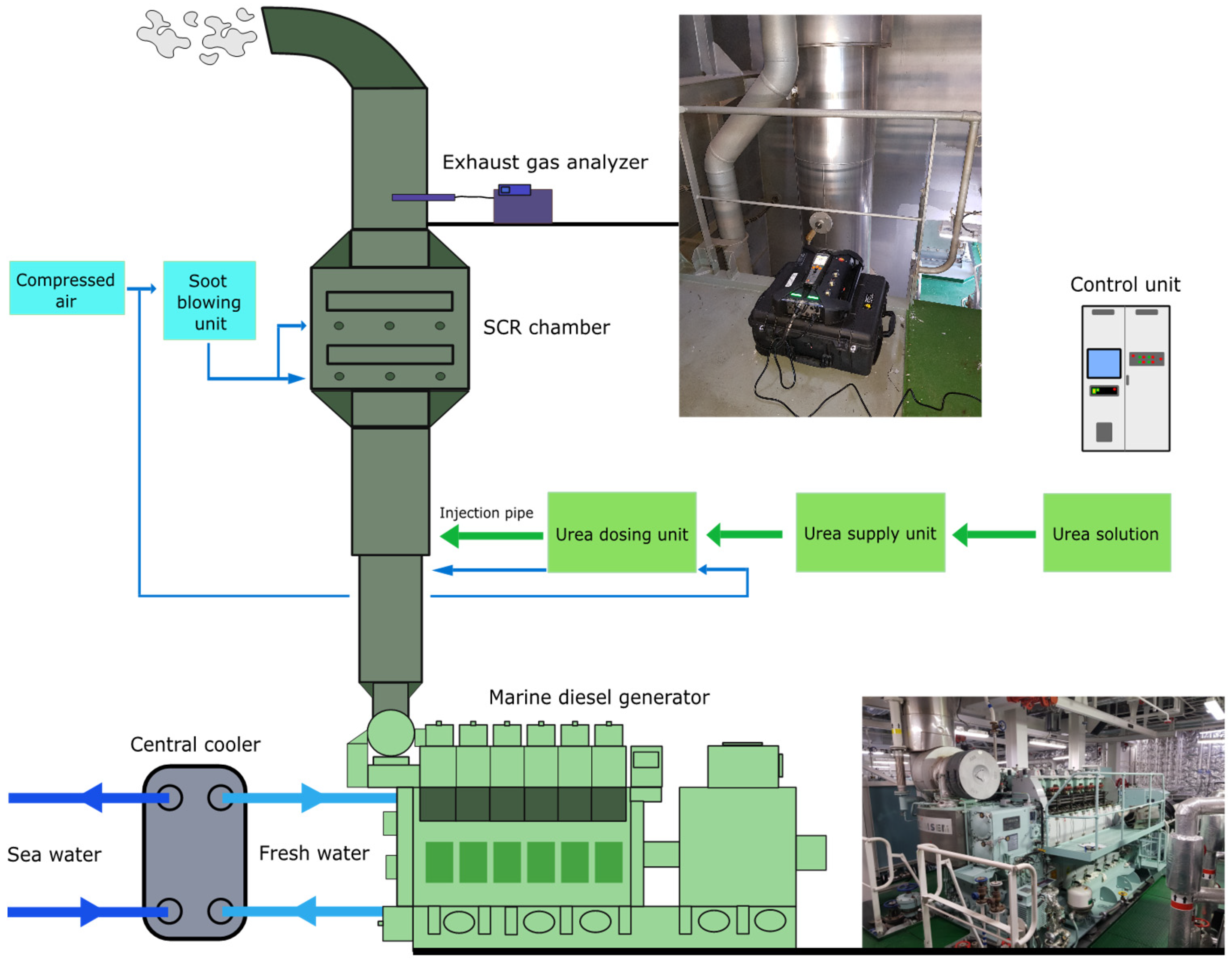
2.1. Description of Machinery and System
2.1.1. G/E and Cooling System
2.1.2. SCR
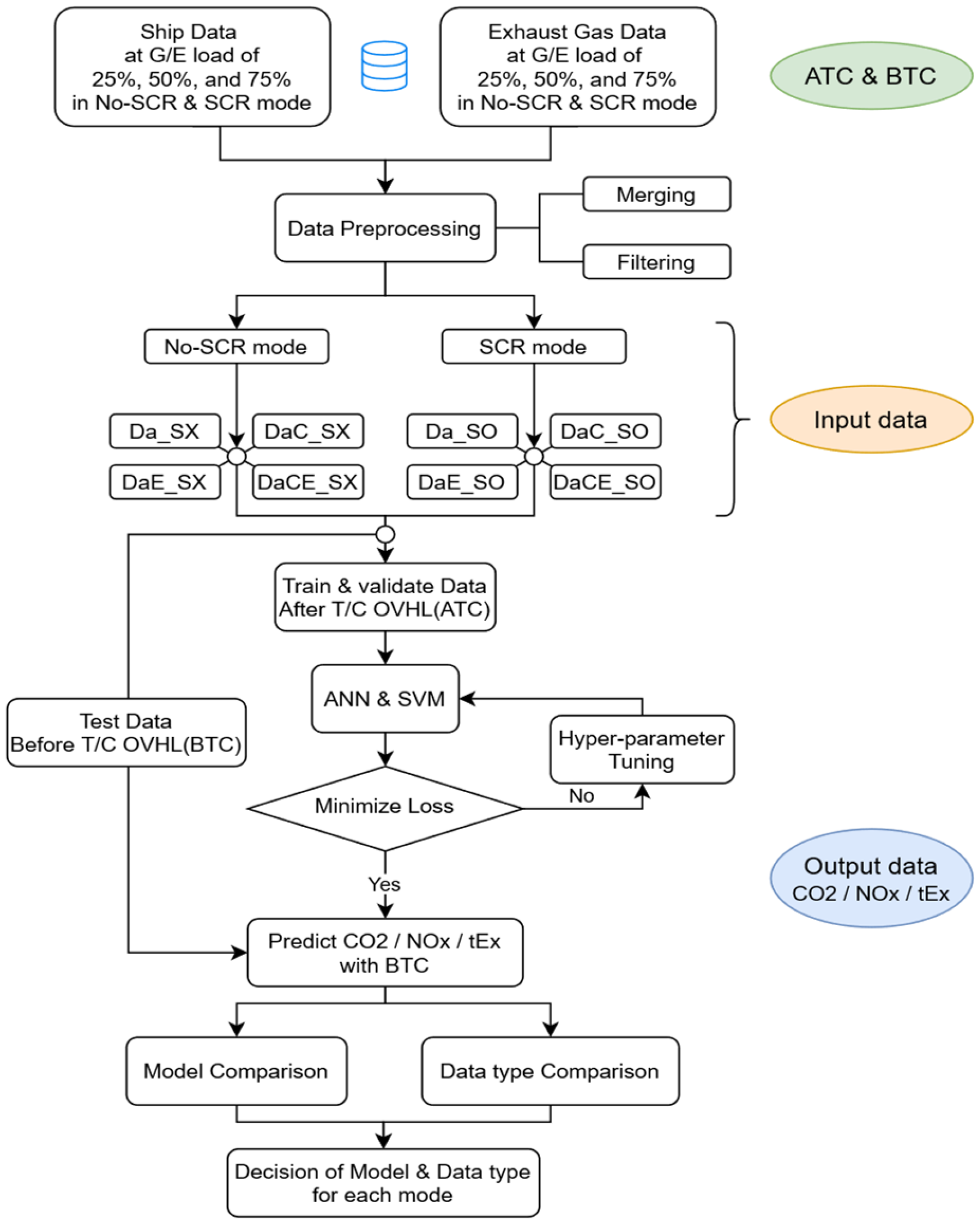
2.2. Description of Workflow
2.2.1. Overview of the Training Sequence
2.2.2. Data Acquisition
2.2.3. Data Preprocessing and Dataset Generation
3. Theory/Modeling
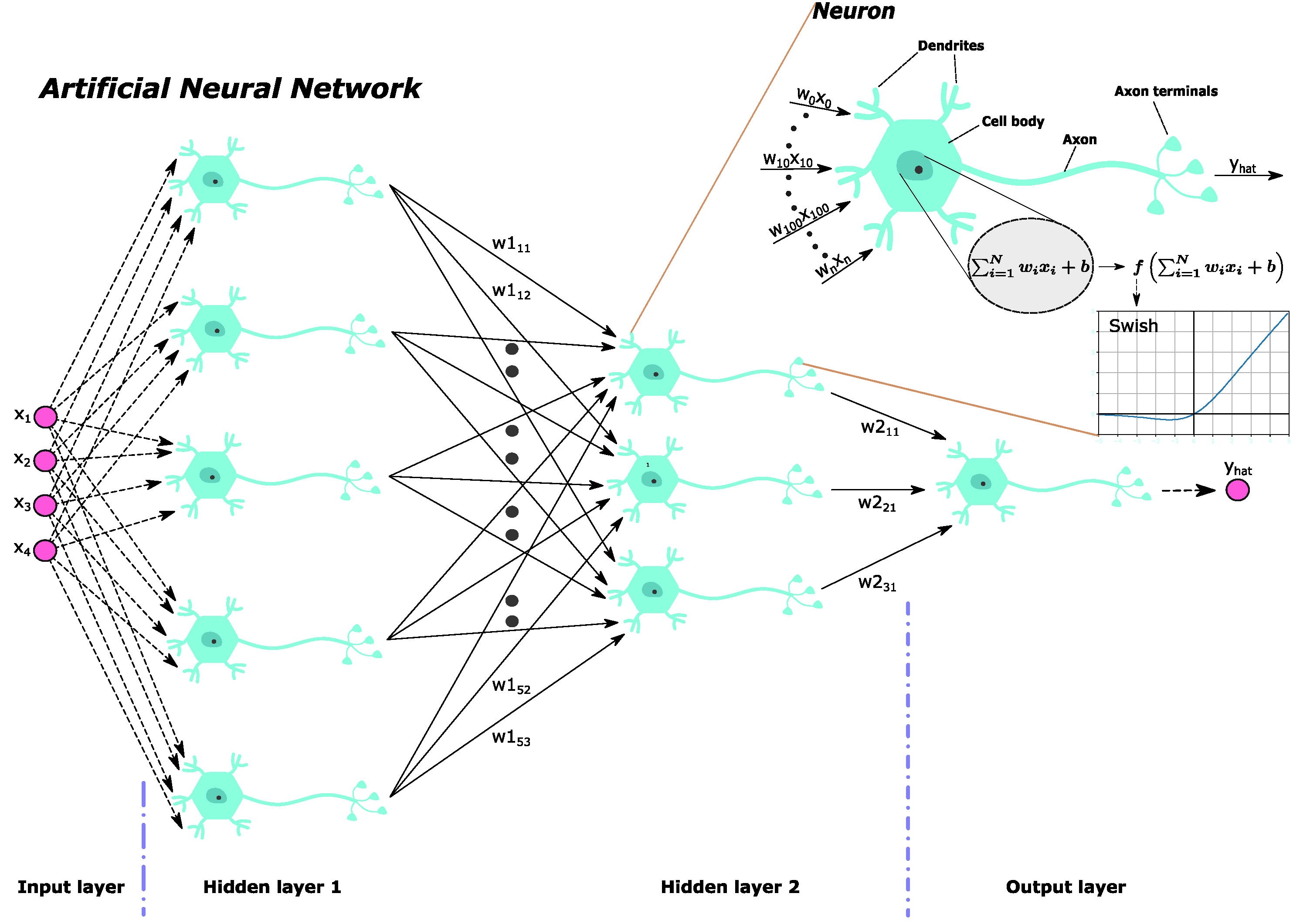
3.1. Artificial Neural Network
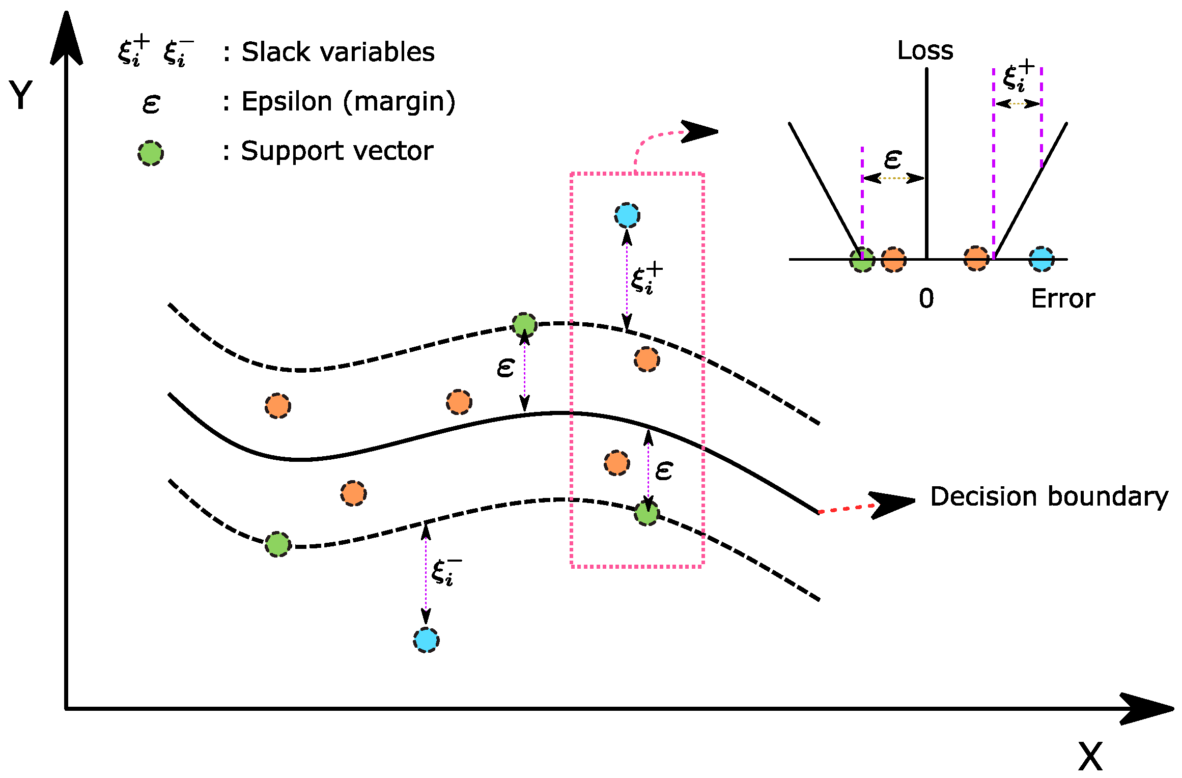
3.2. SVM
3.3. Performance Measurement Metrics
4. Results and Discussion
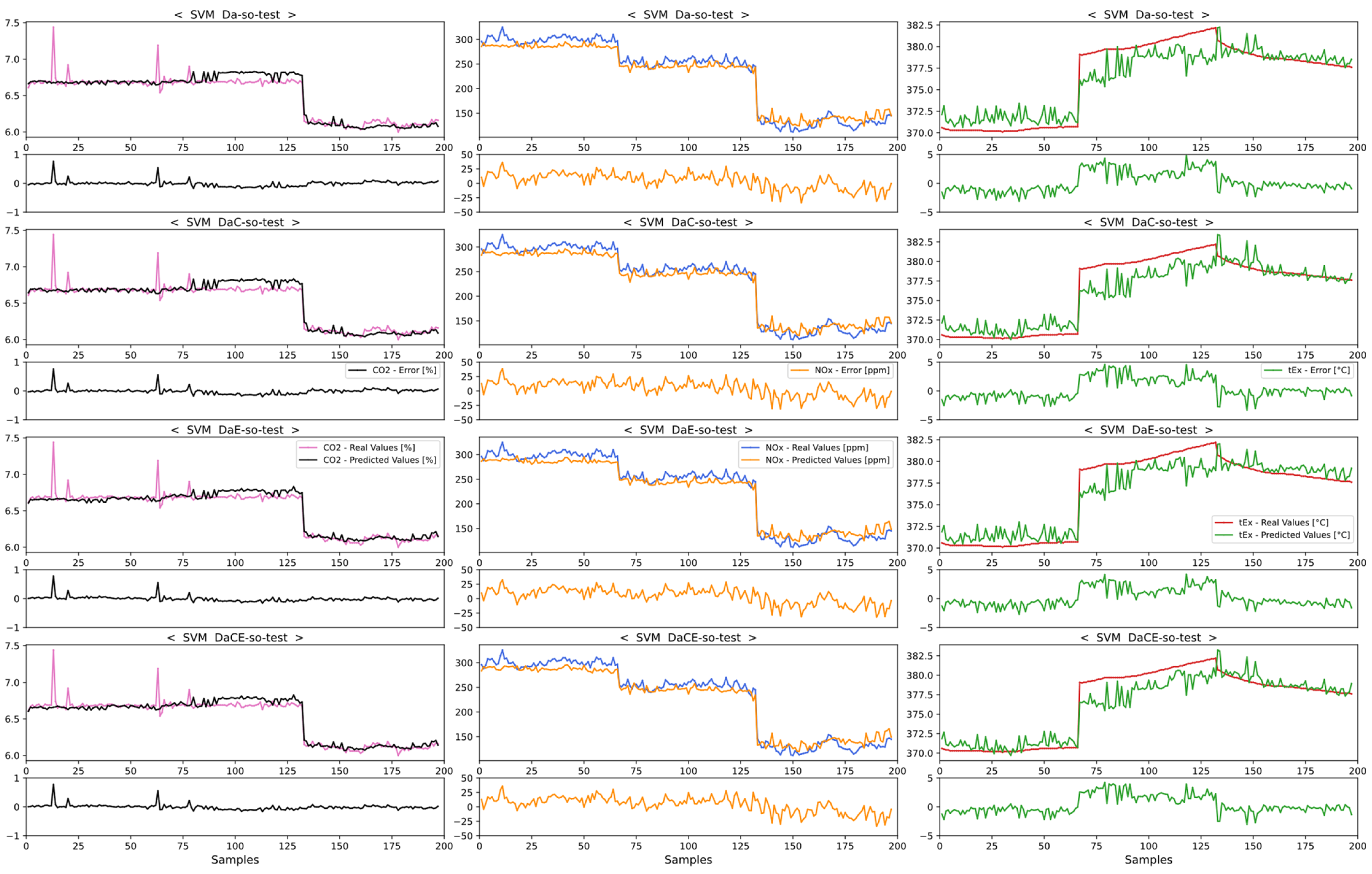
4.1. Comparison of Emission Predictions of ANN and SVM Models for the No-SCR Mode
4.1.1. Comparison of Dataset Types for the No-SCR Mode
4.1.2. Comparison of Model Performances with the No-SCR Mode
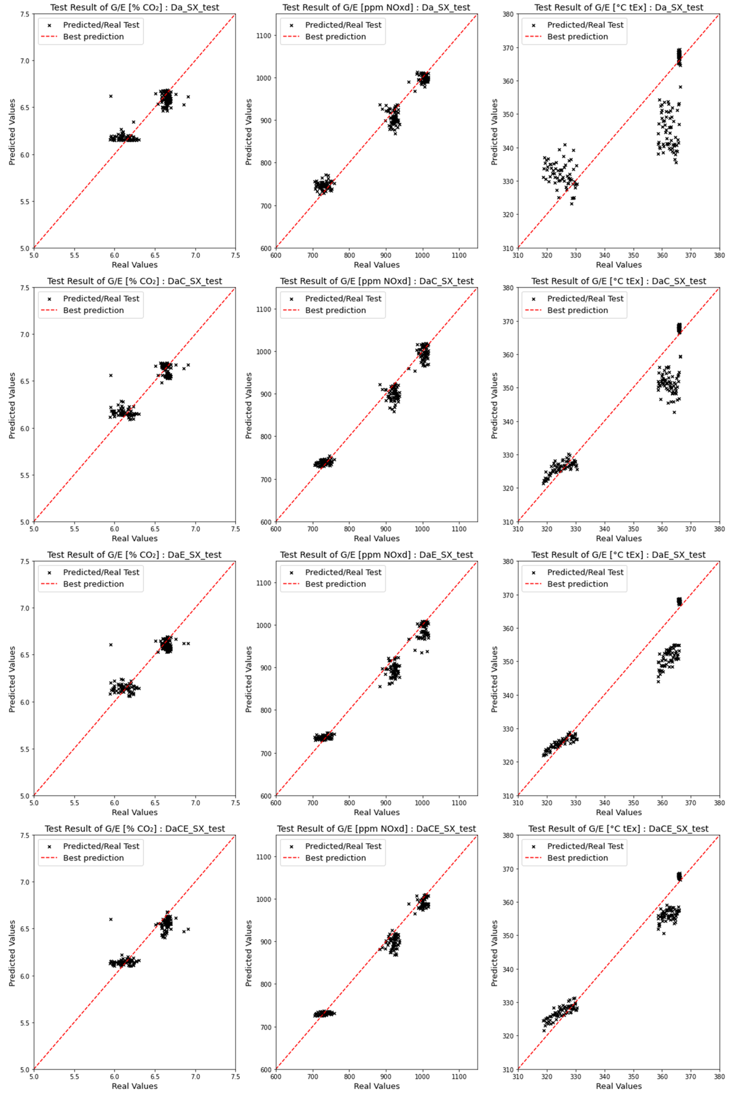
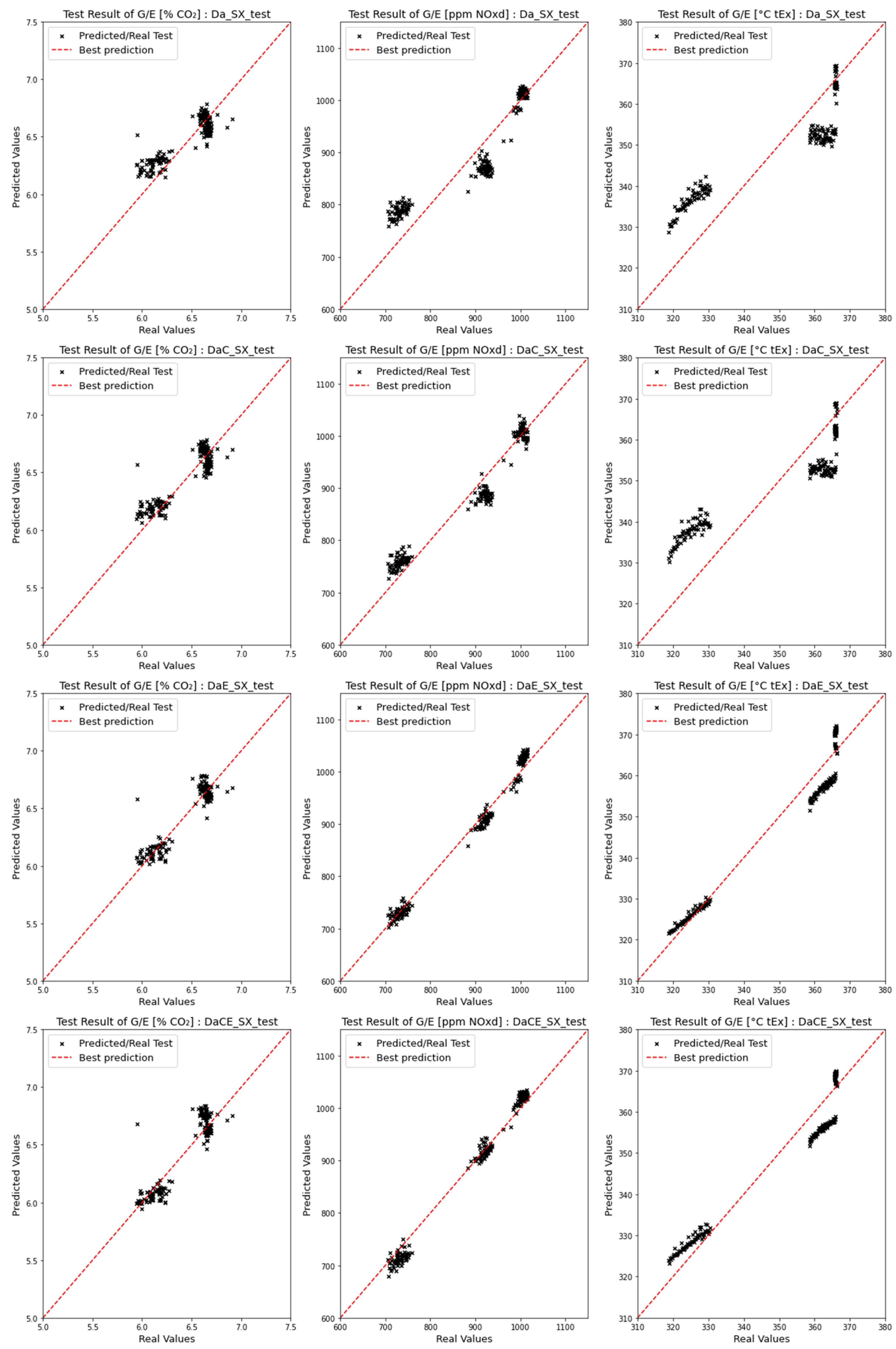
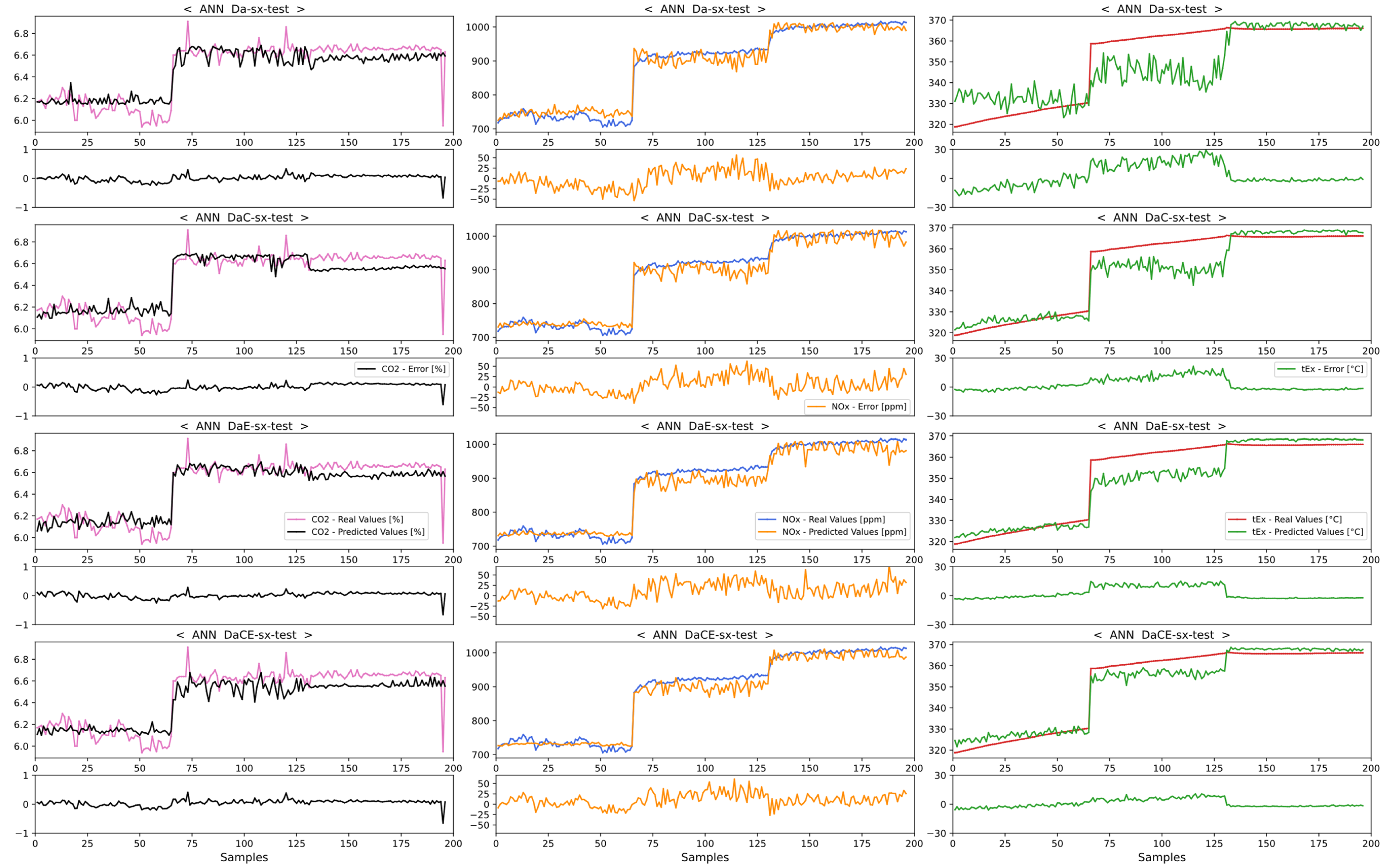
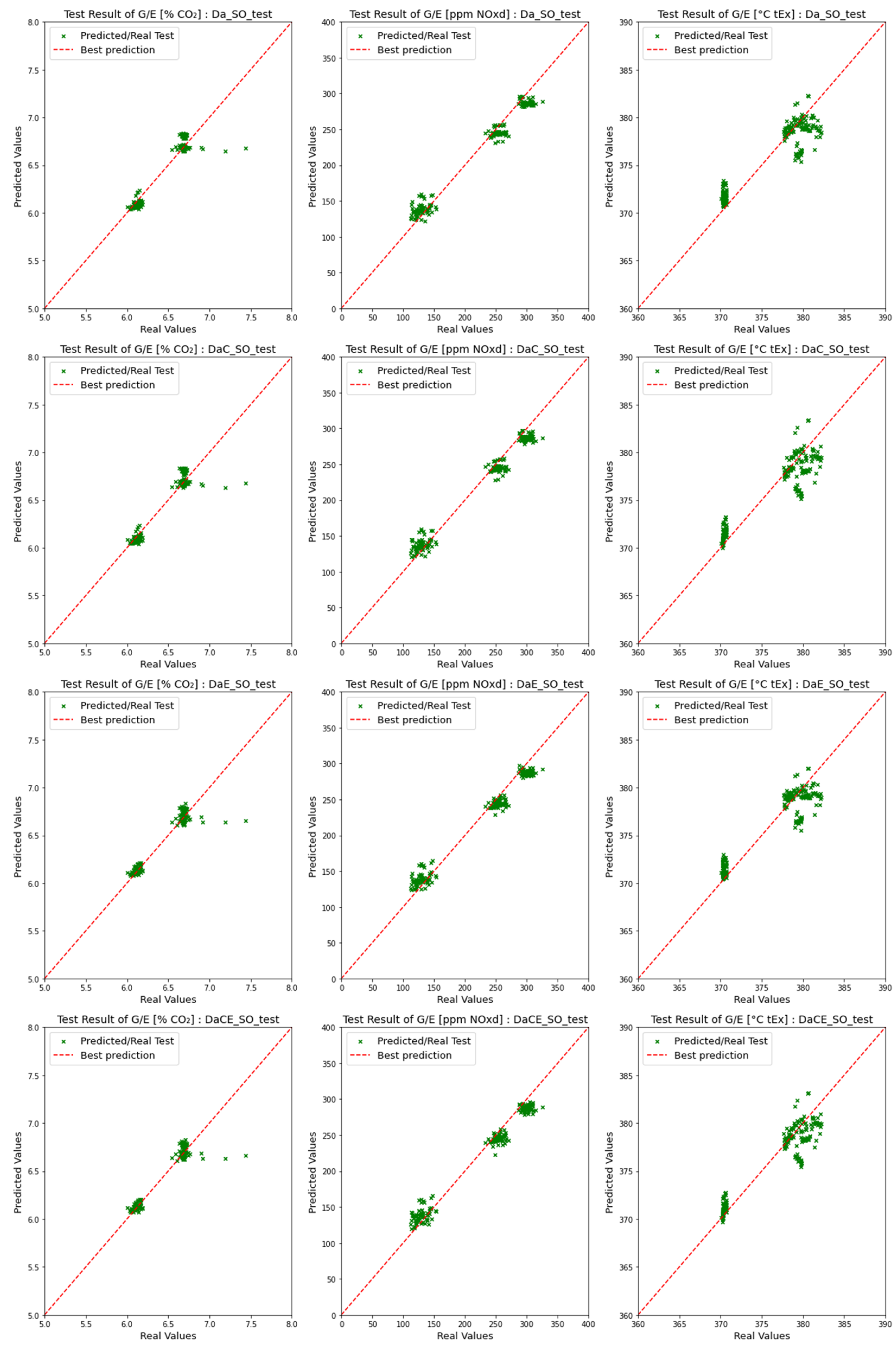
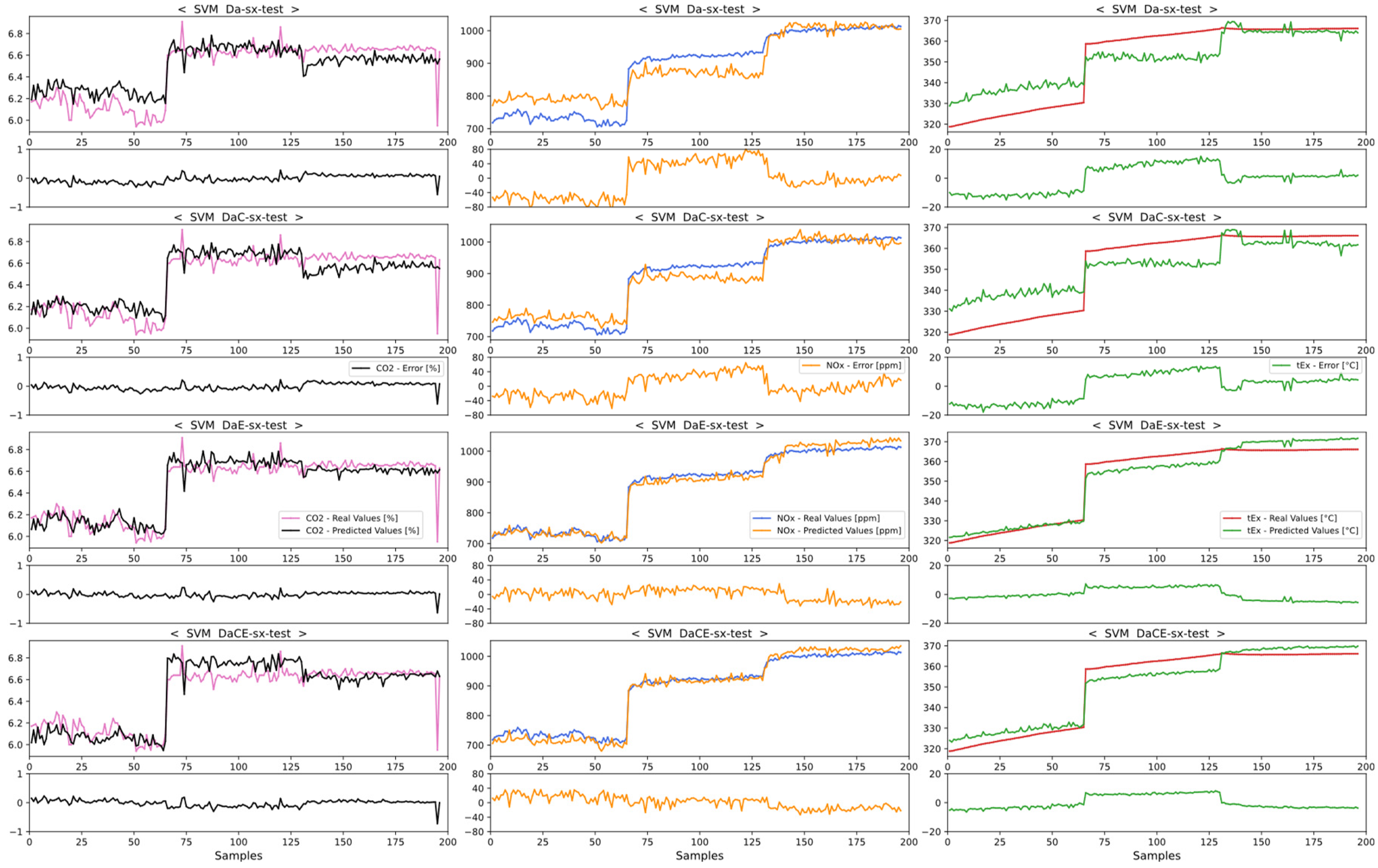
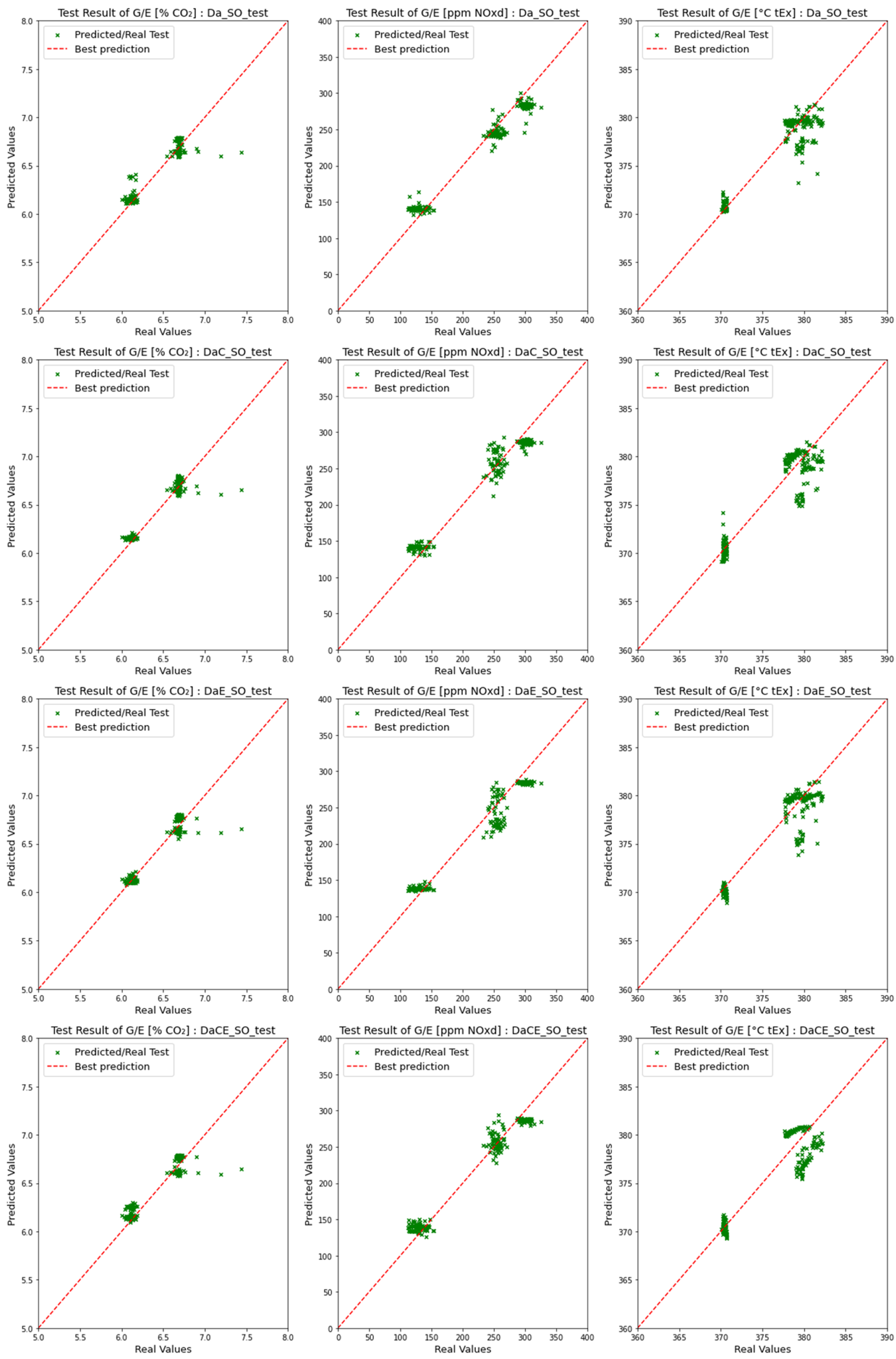
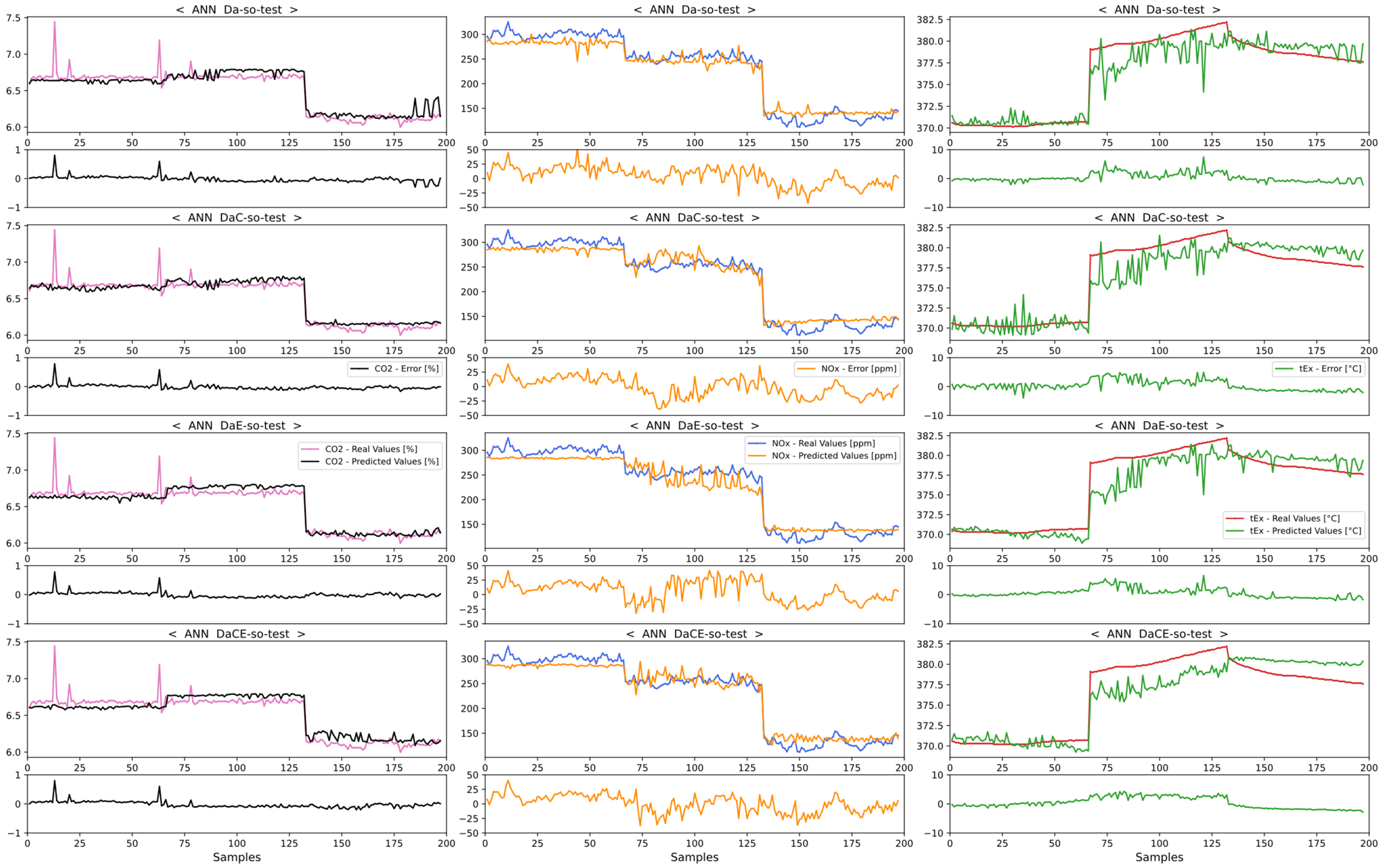
4.2. Comparison of Emission Predictions of ANN and SVM Models with the SCR Mode
4.2.1. Comparison of Dataset Type with the SCR Mode
4.2.2. Comparison of Model Performance in the SCR Mode
5. Conclusions
Author Contributions
Funding
Institutional Review Board Statement
Informed Consent Statement
Data Availability Statement
Conflicts of Interest
Nomenclature
| ATC | After turbocharger overhaul data | R2 | Coefficient of determination |
| BN | Biological neuron | RBF | Gaussian radial basis function |
| BNN | Biological neural network | ReLU | Rectified linear unit |
| BTC | Before turbocharger overhaul data | RMSE | Root-mean-squared error |
| CFW | Cooling freshwater | rpm | Revolutions per minute |
| CI | Compression ignition | SI | Spark ignition |
| CRDI | Common rail direct injection | SVC | Support vector classification |
| DNN | Deep neural network | SVR | Support vector regression |
| F.O | Fuel oil | T/C | Turbocharger |
| GEP | Gene expression programming | tEx | Funnel exhaust gas temperature |
| HCNG | Hydrogen-enriched compressed natural gas | XOR | Exclusive or |
| L.O | Lube oil | Pearson correlation coefficient (Pearson r) | |
| L.T | Low temperature | Actual values | |
| MAE | Mean absolute error | Average of actual values | |
| MAPE | Mean absolute percentage error | Predicted values | |
| MLP | Multiple layer perceptron | Average of predicted values |
References
- UNCTAD. Review of Maritime Transport 2021; UNCTAD: Geneva, Switzerland, 2021. [Google Scholar]
- IMO. Fourth IMO GHG Study 2020 Full Report; IMO: London, UK, 2021. [Google Scholar]
- Chen, J.; Fei, Y.; Wan, Z. The Relationship between the Development of Global Maritime Fleets and GHG Emission from Shipping. J. Environ. Manag. 2019, 242, 31–39. [Google Scholar] [CrossRef] [PubMed]
- Boningari, T.; Smirniotis, P.G. Impact of Nitrogen Oxides on the Environment and Human Health: Mn-Based Materials for the NOx Abatement. Curr. Opin. Chem. Eng. 2016, 13, 133–141. [Google Scholar] [CrossRef]
- Viana, M.; Hammingh, P.; Colette, A.; Querol, X.; Degraeuwe, B.; de Vlieger, I.; van Aardenne, J. Impact of Maritime Transport Emissions on Coastal Air Quality in Europe. Atmos. Environ. 2014, 90, 96–105. [Google Scholar] [CrossRef]
- ABS. ABS Advisory on Nox Tier Iii Compliance; ABS: Houston, TX, USA, 2020. [Google Scholar]
- Ni, P.; Wang, X.; Li, H. A Review on Regulations, Current Status, Effects and Reduction Strategies of Emissions for Marine Diesel Engines. Fuel 2020, 279, 118477. [Google Scholar] [CrossRef]
- Liu, J.; Wang, H. Machine Learning Assisted Modeling of Mixing Timescale for LES/PDF of High-Karlovitz Turbulent Premixed Combustion. Combust. Flame 2022, 238, 111895. [Google Scholar] [CrossRef]
- Adams, D.; Oh, D.H.; Kim, D.W.; Lee, C.H.; Oh, M. Prediction of SOx–NOx Emission from a Coal-Fired CFB Power Plant with Machine Learning: Plant Data Learned by Deep Neural Network and Least Square Support Vector Machine. J. Clean. Prod. 2020, 270, 122310. [Google Scholar] [CrossRef]
- Wang, X.; Liu, W.; Wang, Y.; Yang, G. A Hybrid NOx Emission Prediction Model Based on CEEMDAN and AM-LSTM. Fuel 2021, 310, 122486. [Google Scholar] [CrossRef]
- Zhai, Y.; Ding, X.; Jin, X.; Zhao, L. Adaptive LSSVM Based Iterative Prediction Method for NOx Concentration Prediction in Coal-Fired Power Plant Considering System Delay. Appl. Soft Comput. J. 2020, 89, 106070. [Google Scholar] [CrossRef]
- Tan, Y.; Zhang, J.; Tian, H.; Jiang, D.; Guo, L.; Wang, G.; Lin, Y. Multi-Label Classification for Simultaneous Fault Diagnosis of Marine Machinery: A Comparative Study. Ocean Eng. 2021, 239, 109723. [Google Scholar] [CrossRef]
- Quintanilha, I.M.; Elias, V.R.M.; da Silva, F.B.; Fonini, P.A.M.; da Silva, E.A.B.; Netto, S.L.; Apolinário, J.A.; de Campos, M.L.R.; Martins, W.A.; Wold, L.E.; et al. A Fault Detector/Classifier for Closed-Ring Power Generators Using Machine Learning. Reliab. Eng. Syst. Saf. 2021, 212, 107614. [Google Scholar] [CrossRef]
- Wang, X.; Cai, Y.; Li, A.; Zhang, W.; Yue, Y.; Ming, A. Intelligent Fault Diagnosis of Diesel Engine via Adaptive VMD-Rihaczek Distribution and Graph Regularized Bi-Directional NMF. Meas. J. Int. Meas. Confed. 2021, 172, 108823. [Google Scholar] [CrossRef]
- Castresana, J.; Gabiña, G.; Martin, L.; Uriondo, Z. Comparative Performance and Emissions Assessments of a Single-Cylinder Diesel Engine Using Artificial Neural Network and Thermodynamic Simulation. Appl. Therm. Eng. 2021, 185, 116343. [Google Scholar] [CrossRef]
- Tuan Hoang, A.; Nižetić, S.; Chyuan Ong, H.; Tarelko, W.; Viet Pham, V.; Hieu Le, T.; Quang Chau, M.; Phuong Nguyen, X. A Review on Application of Artificial Neural Network (ANN) for Performance and Emission Characteristics of Diesel Engine Fueled with Biodiesel-Based Fuels. Sustain. Energy Technol. Assess. 2021, 47, 101416. [Google Scholar] [CrossRef]
- Ouyang, T.; Huang, G.; Su, Z.; Xu, J.; Zhou, F.; Chen, N. Design and Optimisation of an Advanced Waste Heat Cascade Utilisation System for a Large Marine Diesel Engine. J. Clean. Prod. 2020, 273, 123057. [Google Scholar] [CrossRef]
- Zhou, H.; Yang, W.; Sun, L.; Jing, X.; Li, G.; Cao, L. Reliability Optimization of Process Parameters for Marine Diesel Engine Block Hole System Machining Using Improved PSO. Sci. Rep. 2021, 11, 21983. [Google Scholar] [CrossRef]
- Asalapuram, V.S.; Khan, I.; Rao, K. A Novel Architecture for Condition Based Machinery Health Monitoring on Marine Vessels Using Deep Learning and Edge Computing. In Proceedings of the 2019 22nd IEEE International Symposium on Measurement and Control in Robotics: Robotics for the Benefit of Humanity (ISMCR 2019), Houston, TX, USA, 19–21 September 2019. [Google Scholar]
- Lazakis, I.; Gkerekos, C.; Theotokatos, G. Investigating an SVM-Driven, One-Class Approach to Estimating Ship Systems Condition. Ships Offshore Struct. 2019, 14, 432–441. [Google Scholar] [CrossRef]
- Tang, R.; Li, X.; Lai, J. A Novel Optimal Energy-Management Strategy for a Maritime Hybrid Energy System Based on Large-Scale Global Optimization. Appl. Energy 2018, 228, 254–264. [Google Scholar] [CrossRef]
- Uyanık, T.; Karatuğ, Ç.; Arslanoğlu, Y. Machine Learning Approach to Ship Fuel Consumption: A Case of Container Vessel. Transp. Res. Part D Transp. Environ. 2020, 84, 102389. [Google Scholar] [CrossRef]
- Duan, H.; Huang, Y.; Mehra, R.K.; Song, P.; Ma, F. Study on Influencing Factors of Prediction Accuracy of Support Vector Machine (SVM) Model for NOx Emission of a Hydrogen Enriched Compressed Natural Gas Engine. Fuel 2018, 234, 954–964. [Google Scholar] [CrossRef]
- Yusri, I.M.; Abdul Majeed, A.P.P.; Mamat, R.; Ghazali, M.F.; Awad, O.I.; Azmi, W.H. A Review on the Application of Response Surface Method and Artificial Neural Network in Engine Performance and Exhaust Emissions Characteristics in Alternative Fuel. Renew. Sustain. Energy Rev. 2018, 90, 665–686. [Google Scholar] [CrossRef]
- Shivakumar; Srinivasa Pai, P.; Shrinivasa Rao, B.R. Artificial Neural Network Based Prediction of Performance and Emission Characteristics of a Variable Compression Ratio CI Engine Using WCO as a Biodiesel at Different Injection Timings. Appl. Energy 2011, 88, 2344–2354. [Google Scholar] [CrossRef]
- Najafi, G.; Ghobadian, B.; Tavakoli, T.; Buttsworth, D.R.; Yusaf, T.F.; Faizollahnejad, M. Performance and Exhaust Emissions of a Gasoline Engine with Ethanol Blended Gasoline Fuels Using Artificial Neural Network. Appl. Energy 2009, 86, 630–639. [Google Scholar] [CrossRef]
- Çay, Y.; Korkmaz, I.; Çiçek, A.; Kara, F. Prediction of Engine Performance and Exhaust Emissions for Gasoline and Methanol Using Artificial Neural Network. Energy 2013, 50, 177–186. [Google Scholar] [CrossRef]
- Ganesan, P.; Rajakarunakaran, S.; Thirugnanasambandam, M.; Devaraj, D. Artificial Neural Network Model to Predict the Diesel Electric Generator Performance and Exhaust Emissions. Energy 2015, 83, 115–124. [Google Scholar] [CrossRef]
- Niu, X.; Yang, C.; Wang, H.; Wang, Y. Investigation of ANN and SVM Based on Limited Samples for Performance and Emissions Prediction of a CRDI-Assisted Marine Diesel Engine. Appl. Therm. Eng. 2017, 111, 1353–1364. [Google Scholar] [CrossRef]
- Liu, J.; Huang, Q.; Ulishney, C.; Dumitrescu, C.E. Machine Learning Assisted Prediction of Exhaust Gas Temperature of a Heavy-Duty Natural Gas Spark Ignition Engine. Appl. Energy 2021, 300, 117413. [Google Scholar] [CrossRef]
- Liu, B.; Hu, J.; Yan, F.; Turkson, R.F.; Lin, F. A Novel Optimal Support Vector Machine Ensemble Model for NOX Emissions Prediction of a Diesel Engine. Meas. J. Int. Meas. Confed. 2016, 92, 183–192. [Google Scholar] [CrossRef]
- Fu, J.; Yang, R.; Li, X.; Sun, X.; Li, Y.; Liu, Z.; Zhang, Y.; Sunden, B. Application of Artificial Neural Network to Forecast Engine Performance and Emissions of a Spark Ignition Engine. Appl. Therm. Eng. 2022, 201, 117749. [Google Scholar] [CrossRef]
- Roy, S.; Ghosh, A.; Das, A.K.; Banerjee, R. Development and Validation of a GEP Model to Predict the Performance and Exhaust Emission Parameters of a CRDI Assisted Single Cylinder Diesel Engine Coupled with EGR. Appl. Energy 2015, 140, 52–64. [Google Scholar] [CrossRef]
- Roy, S.; Banerjee, R.; Bose, P.K. Performance and Exhaust Emissions Prediction of a CRDI Assisted Single Cylinder Diesel Engine Coupled with EGR Using Artificial Neural Network. Appl. Energy 2014, 119, 330–340. [Google Scholar] [CrossRef]
- Sekar, R.R. Trends in Diesel Engine Charge Air Cooling. SAE Tech. Pap. 1982, 91, 820284–820688. [Google Scholar]
- Kim, J.H.; Kim, Y.; Lu, W. Prediction of Ice Resistance for Ice-Going Ships in Level Ice Using Artificial Neural Network Technique. Ocean Eng. 2020, 217, 108031. [Google Scholar] [CrossRef]
- McCulloch, W.S.; Pitts, W. A Logical Calculus of the Ideas Immanent in Nervous Activity. Bull. Math. Biophys. 1943, 5, 115–133. [Google Scholar] [CrossRef]
- Rosenblatt, F. The Perceptron: A Probabilistic Model for Information Storage and Organization in the Brain. Psychol. Rev. 1958, 65, 386–408. [Google Scholar] [CrossRef]
- Minsky, M.; Papert, S. Perceptrons; MIT Press: Cambridge, MA, USA, 1969. [Google Scholar]
- Rumelhart, D.E.; Hinton, G.E.; Williams, R.J. Learning Internal Representations by Error Propagation. In Readings in Cognitive Science: A Perspective from Psychology and Artificial Intelligence; Elsevier: Amsterdam, The Netherlands, 2013. [Google Scholar]
- Ramachandran, P.; Zoph, B.; Le, Q.V. Swish: A Self-Gated Activation Function. In Proceedings of the 6th International Conference on Learning Representations (ICLR 2018), Vancouver, BC, Canada, 30 April–3 May 2018. [Google Scholar]
- Glorot, X.; Bengio, Y. Understanding the Difficulty of Training Deep Feedforward Neural Networks. Proc. J. Mach. Learn. Res. 2010, 9, 249–256. [Google Scholar]
- He, K.; Zhang, X.; Ren, S.; Sun, J. Delving Deep into Rectifiers: Surpassing Human-Level Performance on Imagenet Classification. In Proceedings of the 2015 IEEE International Conference on Computer Vision (ICCV), Santiago, Chile, 7–13 December 2015; pp. 1026–1034. [Google Scholar] [CrossRef]
- Dozat, T. Incorporating Nesterov Momentum into Adam. In Proceedings of the ICLR 2016-Workshop Track, San Juan, Puerto Rico, 2–4 May 2016. [Google Scholar]
- Srivastava, N.; Hinton, G.; Krizhevsky, A.; Sutskever, I.; Salakhutdinov, R. Dropout: A Simple Way to Prevent Neural Networks from Overfitting. J. Mach. Learn. Res. 2014, 15, 1929–1958. [Google Scholar]
- Boser, B.E.; Guyon, I.M.; Vapnik, V.N. Training Algorithm for Optimal Margin Classifiers. In Proceedings of the Fifth Annual ACM Workshop on Computational Learning Theory, Pittsburgh, PA, USA, 27–29 July 1992. [Google Scholar]
- Guyon, I.; Boser, B.; Vapnik, V. Automatic Capacity Tuning of Very Large VC-Dimension Classifiers. Adv. Neural Inf. Process. Syst. 1993, 5, 147–155. [Google Scholar]
- Cortes, C.; Vapnik, V. Support-Vector Networks. Mach. Learn. 1995, 20, 273–297. [Google Scholar] [CrossRef]
- Schölkopf, B.; Burges, C.; Vapnik, V. Extracting Support Data for a given Task. In Proceedings of the 1st International Conference on Knowledge Discovery & Data Mining, Montreal, QC, Canada, 20–21 August 1995. [Google Scholar]
- Schölkopf, B.; Burges, C.; Vapnik, V. Incorporating Invariances in Support Vector Learning Machines. In Proceedings of the Lecture Notes in Computer Science (Including Subseries Lecture Notes in Artificial Intelligence and Lecture Notes in Bioinformatics), Bochum, Germany, 16–19 July 1996; Springer: Berlin/Heidelberg, Germany, 1996; Volume 1112 LNCS. [Google Scholar]
- Vapnik, V.; Golowich, S.E.; Smola, A. Support Vector Method for Function Approximation, Regression Estimation, and Signal Processing. Adv. Neural Inf. Process. Syst. 1996, 9, 281–287. [Google Scholar]
- Chi, M.; Feng, R.; Bruzzone, L. Classification of Hyperspectral Remote-Sensing Data with Primal SVM for Small-Sized Training Dataset Problem. Adv. Space Res. 2008, 41, 1793–1799. [Google Scholar] [CrossRef]
- Lee, K.; Chung, Y.; Byun, H. SVM-Based Face Verification with Feature Set of Small Size. Electron. Lett. 2002, 38, 787–789. [Google Scholar] [CrossRef]
- Pal, M.; Foody, G.M. Evaluation of SVM, RVM and SMLR for Accurate Image Classification with Limited Ground Data. IEEE J. Sel. Top. Appl. Earth Obs. Remote Sens. 2012, 5, 1344–1355. [Google Scholar] [CrossRef]
- Géron, A. Hands-On Machine Learning with Scikit-Learn, Keras and TensorFlow: Concepts, Tools, and Techniques to Build Intelligent Systems; O’Reilly Media, Inc.: Sebastopol, CA, USA, 2019. [Google Scholar]
- Noble, W.S. What Is a Support Vector Machine? Nat. Biotechnol. 2006, 24, 1565–1567. [Google Scholar] [CrossRef]
- Drucker, H.; Surges, C.J.C.; Kaufman, L.; Smola, A.; Vapnik, V. Support Vector Regression Machines. Adv. Neural Inf. Process. Syst. 1996, 9, 155–161. [Google Scholar]
- Smola, A.J.; Schölkopf, B. A Tutorial on Support Vector Regression. Stat. Comput. 2004, 14, 199–222. [Google Scholar] [CrossRef]


| Type of Engine | 4-Stroke, Vertical, Direct Injection Single-Acting, and Trunk Piston Type with T/C and Intercooler |
|---|---|
| Cylinder configuration | Inline |
| Number of cylinders | 6 |
| Rated speed | 900 rpm |
| Power per cylinder | 200 kW |
| Cylinder bore | 210 mm |
| Piston stroke | 320 mm |
| Swept volume per cylinder | 11.1 dm3 |
| Mean piston speed | 9.6 m/s |
| Mean effective pressure | 24.1 bar |
| Compression ratio | 17:1 |
| Cylinder firing order | 1–4–2–6–3–5 |
| NOx emission value after the SCR | 2.31 g/kWh |
| Pressure drop across the SCR | ≤150 mmAq |
| Ammonia slip | ≤10 ppm |
| Sulfur content of the fuel oil for SCR operation | ≤0.1% |
| Maximum allowable exhaust gas temperature | ≤400 °C |
| API gravity, 60 °F | 35.6 |
| Specific gravity, 15/4 °C | 0.8464 |
| Flash point | 66.0 °C |
| Sulfur | 0.0340 wt.% |
| Kinematic viscosity | 2.8940 mm2/s |
| Net heat of combustion | 10,220 kcal/kg |
| Gross heat of combustion | 10,891 kcal/kg |
| Flue gas CO2 | ±2% ppm |
| Flue gas NOx | ±2% ppm |
| Exhaust gas temperature | ±0.4 °C (−100 to +200.0 °C) |
| ±1.0 °C (200 to +1370.0 °C) |
| Parameter | Range |
|---|---|
| Common data for all datasets | |
| LO inlet temperature (°C) | 63.98–66.96 |
| Cylinder exhaust gas outlet temperature—average (°C) | 386.07–440.86 |
| FO inlet temperature (°C) | 14.99–19.98 |
| T/C exhaust gas inlet temperature—average (°C) | 422.95–530.89 |
| LO inlet pressure (kg/cm2) | 4.65–4.89 |
| T/C exhaust gas outlet temperature (°C) | 357.9–408.89 |
| FO inlet pressure (kg/cm2) | 6–6.2 |
| Exhaust gas compensation temperature (°C) | 24.96–36 |
| LO filter inlet pressure (kg/cm2) | 5.1–5.3 |
| Charge air outlet temperature (°C) | 36–38 |
| FO filter inlet pressure (kg/cm2) | 6–6.6 |
| Charge air inlet pressure (kg/cm2) | 0.5–2.4 |
| T/C LO inlet pressure (kg/cm2) | 3–3.5 |
| T/C rpm pick-up (rpm) | 22,603.18–40,771.68 |
| Engine rpm pick-up (rpm) | 897–901.98 |
| Additional data for DaC | |
| LT CFW outlet temperature (°C) | 34.97–40.98 |
| LT CFW temperature difference (°C) | 0–5.03 |
| Central CFW cooler temperature difference (°C) | 0.47–1.11 |
| Additional data for DaE | |
| Alternator winding phase temperature-average (°C) | 37.75–65.64 |
| G/E generator current (A) | 336–1186 |
| G/E generator power (kW) | 242–791.7 |
| G/E current phase-average (A) | 331–1176.33 |
| G/E bus net used power (kW) | 341–864 |
| G/E non-drive-end bearing temperature (°C) | 39.18–54.09 |
| Additional data for SCR mode | |
| G/E load to G/E SCR (%) | 23.05–75.32 |
| Urea injection (l/h) | 4.7–14.68 |
| Prediction data | |
| CO2 (%) | 5.48–7.44 |
| NOx (ppm) | 51–1016 |
| tEx (°C) | 158.1–382.2 |
| Hyperparameter | Value |
|---|---|
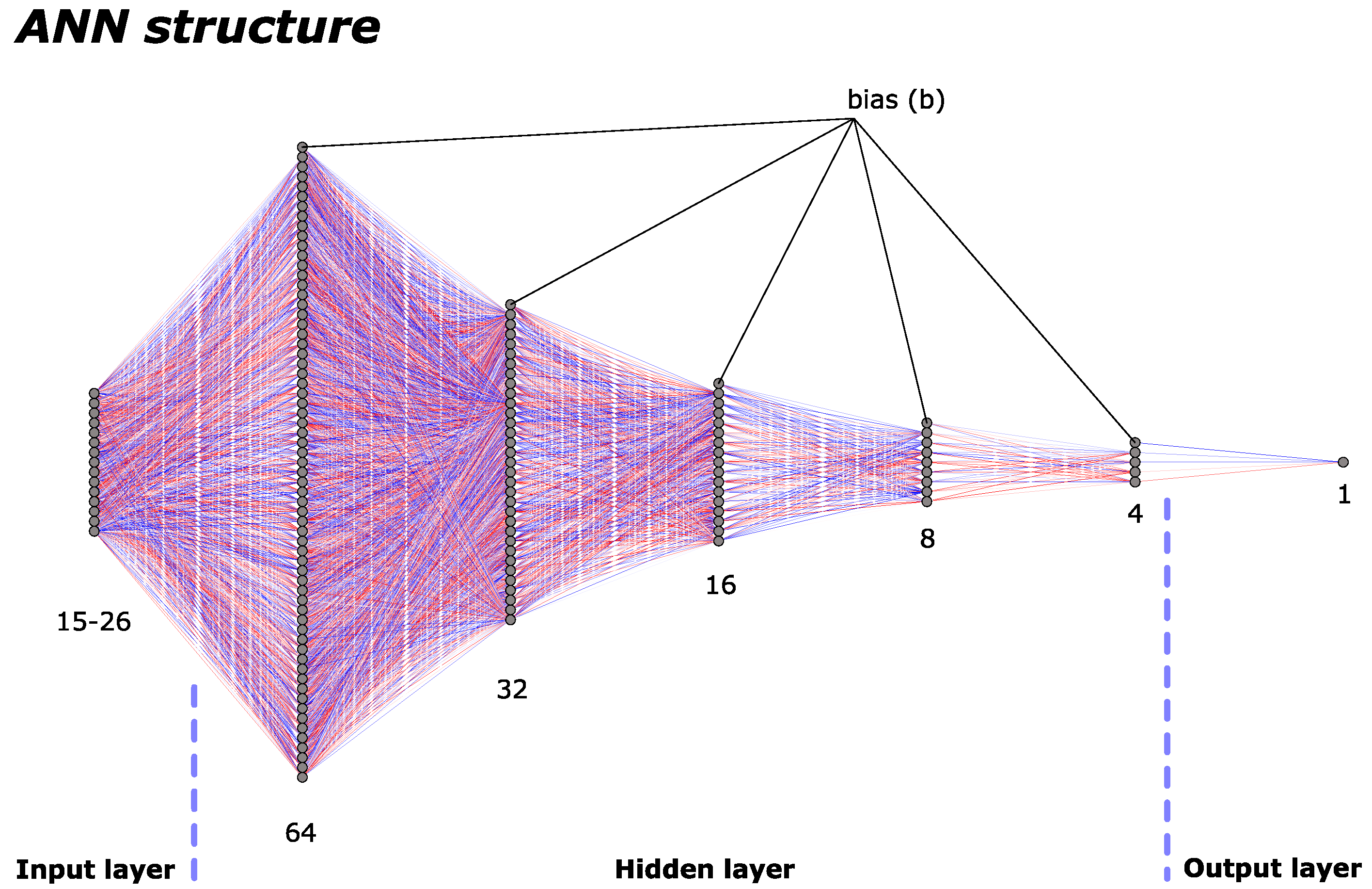
| ANN structure | 64–32–16–8–4–1 |
| Activation function | Swish |
| Kernel initializer | He-uniform |
| Optimizer | Nadam |
| Learning rate for the optimizer | 0.0001 |
| Dropout rate | 10% |
| Patience for early stopping | 300 |
| Epochs | 3000 |
| Batch size | 16 |
| Da-sx | DaC-sx | DaE-sx | DaCE-sx | ||||||||||
| CO2 (%) | NOx (ppm) | tEx (°C) | CO2 (%) | NOx (ppm) | tEx (°C) | CO2 (%) | NOx (ppm) | tEx (°C) | CO2 (%) | NOx (ppm) | tEx (°C) | ||
| (a) | RMSE | 0.0461 | 13.5937 | 5.5857 | 0.0460 | 12.9778 | 5.1007 | 0.0425 | 11.8056 | 5.2933 | 0.0449 | 12.3552 | 4.0531 |
| MAE | 0.0338 | 10.9727 | 4.0019 | 0.0335 | 10.2915 | 3.7966 | 0.0313 | 9.6654 | 3.6559 | 0.0325 | 9.9308 | 2.9179 | |
| MAPE | 0.5474 | 1.3560 | 1.8322 | 0.5434 | 1.2845 | 1.7303 | 0.5071 | 1.1913 | 1.7301 | 0.5259 | 1.2404 | 1.3278 | |
| R2 | 0.9424 | 0.9853 | 0.9918 | 0.9428 | 0.9860 | 0.9923 | 0.9510 | 0.9891 | 0.9915 | 0.9453 | 0.9878 | 0.9955 | |
| Pearson r | 0.9735 | 0.9950 | 0.9977 | 0.9740 | 0.9960 | 0.9980 | 0.9769 | 0.9961 | 0.9986 | 0.9755 | 0.9966 | 0.9989 | |
| Da-sx-test | DaC-sx-test | DaE-sx-test | DaCE-sx-test | ||||||||||
| CO2 (%) | NOx (ppm) | tEx (°C) | CO2 (%) | NOx (ppm) | tEx (°C) | CO2 (%) | NOx (ppm) | tEx (°C) | CO2 (%) | NOx (ppm) | tEx (°C) | ||
| (b) | RMSE | 0.1208 | 25.8067 | 6.7677 | 0.1148 | 26.8612 | 7.0220 | 0.1010 | 21.3484 | 5.1222 | 0.1093 | 20.2085 | 5.5835 |
| MAE | 0.0915 | 20.1967 | 5.2798 | 0.0883 | 20.5117 | 5.2452 | 0.0756 | 16.1402 | 4.1195 | 0.0841 | 16.0501 | 4.4798 | |
| MAPE | 1.4360 | 2.3328 | 1.5056 | 1.3834 | 2.3573 | 1.4881 | 1.1810 | 1.8805 | 1.1692 | 1.3139 | 1.8724 | 1.2706 | |
| R2 | 0.7846 | 0.9477 | 0.8583 | 0.8075 | 0.9413 | 0.8491 | 0.8498 | 0.9637 | 0.9155 | 0.8245 | 0.9653 | 0.9042 | |
| Pearson r | 0.9090 | 0.9795 | 0.9327 | 0.9213 | 0.9773 | 0.9340 | 0.9335 | 0.9858 | 0.9621 | 0.9266 | 0.9866 | 0.9550 | |
| (c) | RMSE | 0.1100 | 20.6742 | 11.8977 | 0.1083 | 20.7300 | 7.1590 | 0.0991 | 23.8558 | 6.7880 | 0.1162 | 19.1140 | 4.2768 |
| MAE | 0.0835 | 16.5848 | 8.9862 | 0.0872 | 16.2398 | 5.2717 | 0.0742 | 18.9137 | 5.1237 | 0.0929 | 14.9196 | 3.5232 | |
| MAPE | 1.3052 | 1.9477 | 2.5613 | 1.3618 | 1.8357 | 1.4758 | 1.1608 | 2.1030 | 1.4325 | 1.4376 | 1.6747 | 0.9975 | |
| R2 | 0.8242 | 0.9673 | 0.5905 | 0.8294 | 0.9671 | 0.8518 | 0.8573 | 0.9564 | 0.8667 | 0.8036 | 0.9720 | 0.9471 | |
| Pearson r | 0.9229 | 0.9858 | 0.7856 | 0.9162 | 0.9858 | 0.9342 | 0.9326 | 0.9865 | 0.9417 | 0.9335 | 0.9910 | 0.9752 | |
| Da-sx | DaC-sx | DaE-sx | DaCE-sx | ||||||||||
| CO2 (%) | NOx (ppm) | tEx (°C) | CO2 (%) | NOx (ppm) | tEx (°C) | CO2 (%) | NOx (ppm) | tEx (°C) | CO2 (%) | NOx (ppm) | tEx (°C) | ||
| (a) | RMSE | 0.0356 | 8.9050 | 2.2663 | 0.0336 | 6.8926 | 2.1422 | 0.0343 | 5.9282 | 0.6333 | 0.0324 | 6.0193 | 0.4150 |
| MAE | 0.0274 | 6.3848 | 1.6711 | 0.0272 | 5.0855 | 1.4682 | 0.0266 | 4.7832 | 0.3586 | 0.0264 | 5.0455 | 0.3143 | |
| MAPE | 0.4421 | 0.7546 | 0.6191 | 0.4366 | 0.5960 | 0.5583 | 0.4283 | 0.5672 | 0.1548 | 0.4234 | 0.6001 | 0.1324 | |
| R2 | 0.9657 | 0.9939 | 0.9987 | 0.9695 | 0.9963 | 0.9988 | 0.9682 | 0.9973 | 0.9999 | 0.9716 | 0.9972 | 1.0000 | |
| Pearson r | 0.9829 | 0.9970 | 0.9994 | 0.9851 | 0.9982 | 0.9994 | 0.9854 | 0.9987 | 1.0000 | 0.9877 | 0.9986 | 1.0000 | |
| Da-sx-test | DaC-sx-test | DaE-sx-test | DaCE-sx-test | ||||||||||
| CO2 (%) | NOx (ppm) | tEx (°C) | CO2 (%) | NOx (ppm) | tEx (°C) | CO2 (%) | NOx (ppm) | tEx (°C) | CO2 (%) | NOx (ppm) | tEx (°C) | ||
| (b) | RMSE | 0.1312 | 45.9671 | 8.9578 | 0.1136 | 28.7961 | 9.5169 | 0.0901 | 15.6995 | 4.1195 | 0.1137 | 17.1088 | 4.5839 |
| MAE | 0.1073 | 39.2833 | 7.6497 | 0.0936 | 24.9758 | 8.4966 | 0.0659 | 13.5417 | 3.5823 | 0.0836 | 14.5928 | 4.1775 | |
| MAPE | 1.6889 | 4.7777 | 2.2293 | 1.4584 | 2.9362 | 2.4750 | 1.0243 | 1.4900 | 0.9989 | 1.2924 | 1.7120 | 1.1871 | |
| R2 | 0.7499 | 0.8382 | 0.7679 | 0.8124 | 0.9365 | 0.7380 | 0.8819 | 0.9811 | 0.9509 | 0.8119 | 0.9776 | 0.9392 | |
| Pearson r | 0.8995 | 0.9243 | 0.9199 | 0.9058 | 0.9711 | 0.9276 | 0.9399 | 0.9920 | 0.9754 | 0.9303 | 0.9962 | 0.9712 | |
| Da-so | DaC-so | DaE-so | DaCE-so | ||||||||||
| CO2 (%) | NOx (ppm) | tEx (°C) | CO2 (%) | NOx (ppm) | tEx (°C) | CO2 (%) | NOx (ppm) | tEx (°C) | CO2 (%) | NOx (ppm) | tEx (°C) | ||
| (a) | RMSE | 0.0498 | 13.3101 | 0.7196 | 0.0481 | 13.8279 | 0.6893 | 0.0478 | 13.0547 | 0.3538 | 0.0471 | 13.7466 | 0.3843 |
| MAE | 0.0351 | 9.6977 | 0.5599 | 0.0345 | 10.0285 | 0.5240 | 0.0346 | 9.4762 | 0.2760 | 0.0342 | 9.8260 | 0.3080 | |
| MAPE | 0.5633 | 8.6440 | 0.1502 | 0.5539 | 8.6388 | 0.1407 | 0.5545 | 8.4854 | 0.0738 | 0.5486 | 8.7009 | 0.0825 | |
| R2 | 0.9479 | 0.9699 | 0.9701 | 0.9514 | 0.9675 | 0.9725 | 0.9519 | 0.9710 | 0.9928 | 0.9534 | 0.9679 | 0.9910 | |
| Pearson r | 0.9757 | 0.9867 | 0.9880 | 0.9772 | 0.9848 | 0.9909 | 0.9773 | 0.9877 | 0.9972 | 0.9780 | 0.9857 | 0.9972 | |
| Da-so-test | DaC-so-test | DaE-so-test | DaCE-so-test | ||||||||||
| CO2 (%) | NOx (ppm) | tEx (°C) | CO2 (%) | NOx (ppm) | tEx (°C) | CO2 (%) | NOx (ppm) | tEx (°C) | CO2 (%) | NOx (ppm) | tEx (°C) | ||
| (b) | RMSE | 0.1036 | 18.5344 | 1.7806 | 0.1015 | 20.2399 | 1.7621 | 0.1017 | 19.6393 | 1.8163 | 0.1047 | 19.0223 | 1.8988 |
| MAE | 0.0698 | 15.1720 | 1.2828 | 0.0682 | 16.1593 | 1.4040 | 0.0678 | 16.4335 | 1.4341 | 0.0707 | 15.2021 | 1.5524 | |
| MAPE | 1.0647 | 7.6687 | 0.3393 | 1.0362 | 8.1386 | 0.3716 | 1.0283 | 8.1405 | 0.3793 | 1.0766 | 7.6966 | 0.4103 | |
| R2 | 0.8669 | 0.9315 | 0.8339 | 0.8725 | 0.9202 | 0.8407 | 0.8713 | 0.9245 | 0.8322 | 0.8641 | 0.9286 | 0.8166 | |
| Pearson r | 0.9350 | 0.9768 | 0.9197 | 0.9361 | 0.9674 | 0.9205 | 0.9348 | 0.9752 | 0.9179 | 0.9322 | 0.9699 | 0.9086 | |
| (c) | RMSE | 0.1093 | 16.7953 | 1.5430 | 0.0954 | 16.3705 | 1.8551 | 0.0998 | 18.9179 | 1.7513 | 0.1138 | 15.1043 | 1.9636 |
| MAE | 0.0713 | 14.0085 | 1.0606 | 0.0590 | 13.8268 | 1.4716 | 0.0671 | 16.3756 | 1.2498 | 0.0848 | 12.5964 | 1.6660 | |
| MAPE | 1.0901 | 6.9846 | 0.2800 | 0.8975 | 6.9991 | 0.3892 | 1.0114 | 7.6940 | 0.3303 | 1.2954 | 6.3993 | 0.4401 | |
| R2 | 0.8526 | 0.9462 | 0.8795 | 0.8877 | 0.9489 | 0.8258 | 0.8772 | 0.9318 | 0.8448 | 0.8404 | 0.9565 | 0.8049 | |
| Pearson r | 0.9262 | 0.9867 | 0.9411 | 0.9447 | 0.9796 | 0.9155 | 0.9378 | 0.9764 | 0.9291 | 0.9207 | 0.9828 | 0.9031 | |
| Da-so | DaC-so | DaE-so | DaCE-so | ||||||||||
| CO2 (%) | NOx (ppm) | tEx (°C) | CO2 (%) | NOx (ppm) | tEx (°C) | CO2 (%) | NOx (ppm) | tEx (°C) | CO2 (%) | NOx (ppm) | tEx (°C) | ||
| (a) | RMSE | 0.0401 | 11.3561 | 1.0949 | 0.0402 | 11.2468 | 1.0645 | 0.0387 | 10.9078 | 0.9494 | 0.0381 | 10.8215 | 0.9516 |
| MAE | 0.0308 | 8.4896 | 0.7926 | 0.0307 | 8.4305 | 0.6722 | 0.0286 | 8.2835 | 0.7048 | 0.0284 | 8.1028 | 0.6140 | |
| MAPE | 0.4979 | 7.6329 | 0.2114 | 0.4959 | 7.5758 | 0.1791 | 0.4628 | 7.4243 | 0.1881 | 0.4593 | 7.3156 | 0.1636 | |
| R2 | 0.9648 | 0.9776 | 0.9267 | 0.9646 | 0.9780 | 0.9307 | 0.9672 | 0.9793 | 0.9449 | 0.9681 | 0.9797 | 0.9446 | |
| Pearson r | 0.9829 | 0.9889 | 0.9647 | 0.9829 | 0.9891 | 0.9670 | 0.9842 | 0.9898 | 0.9733 | 0.9845 | 0.9899 | 0.9736 | |
| Da-so-test | DaC-so-test | DaE-so-test | DaCE-so-test | ||||||||||
| CO2 (%) | NOx (ppm) | tEx (°C) | CO2 (%) | NOx (ppm) | tEx (°C) | CO2 (%) | NOx (ppm) | tEx (°C) | CO2 (%) | NOx (ppm) | tEx (°C) | ||
| (b) | RMSE | 0.0987 | 13.9492 | 1.7759 | 0.0987 | 13.7728 | 1.7947 | 0.0911 | 13.9251 | 1.5729 | 0.0912 | 13.6775 | 1.5688 |
| MAE | 0.0597 | 11.7822 | 1.4015 | 0.0581 | 11.5351 | 1.3697 | 0.0516 | 11.8302 | 1.2459 | 0.0508 | 11.4612 | 1.1570 | |
| MAPE | 0.9014 | 5.8510 | 0.3717 | 0.8757 | 5.7186 | 0.3627 | 0.7772 | 5.9312 | 0.3301 | 0.7636 | 5.7718 | 0.3061 | |
| R2 | 0.8797 | 0.9629 | 0.8404 | 0.8799 | 0.9638 | 0.8370 | 0.8975 | 0.9630 | 0.8748 | 0.8975 | 0.9643 | 0.8754 | |
| Pearson r | 0.9471 | 0.9909 | 0.9309 | 0.9458 | 0.9904 | 0.9271 | 0.9481 | 0.9916 | 0.9429 | 0.9481 | 0.9912 | 0.9431 | |
Publisher’s Note: MDPI stays neutral with regard to jurisdictional claims in published maps and institutional affiliations. |
© 2022 by the authors. Licensee MDPI, Basel, Switzerland. This article is an open access article distributed under the terms and conditions of the Creative Commons Attribution (CC BY) license (https://creativecommons.org/licenses/by/4.0/).
Share and Cite
Park, M.-H.; Lee, C.-M.; Nyongesa, A.J.; Jang, H.-J.; Choi, J.-H.; Hur, J.-J.; Lee, W.-J. Prediction of Emission Characteristics of Generator Engine with Selective Catalytic Reduction Using Artificial Intelligence. J. Mar. Sci. Eng. 2022, 10, 1118. https://doi.org/10.3390/jmse10081118
Park M-H, Lee C-M, Nyongesa AJ, Jang H-J, Choi J-H, Hur J-J, Lee W-J. Prediction of Emission Characteristics of Generator Engine with Selective Catalytic Reduction Using Artificial Intelligence. Journal of Marine Science and Engineering. 2022; 10(8):1118. https://doi.org/10.3390/jmse10081118
Chicago/Turabian StylePark, Min-Ho, Chang-Min Lee, Antony John Nyongesa, Hee-Joo Jang, Jae-Hyuk Choi, Jae-Jung Hur, and Won-Ju Lee. 2022. "Prediction of Emission Characteristics of Generator Engine with Selective Catalytic Reduction Using Artificial Intelligence" Journal of Marine Science and Engineering 10, no. 8: 1118. https://doi.org/10.3390/jmse10081118
APA StylePark, M.-H., Lee, C.-M., Nyongesa, A. J., Jang, H.-J., Choi, J.-H., Hur, J.-J., & Lee, W.-J. (2022). Prediction of Emission Characteristics of Generator Engine with Selective Catalytic Reduction Using Artificial Intelligence. Journal of Marine Science and Engineering, 10(8), 1118. https://doi.org/10.3390/jmse10081118