
Coupling a Parametric Wave Solver into a Hydrodynamic Circulation Model to Improve Efficiency of Nested Estuarine Storm Surge Predictions


Abstract
:1. Introduction
1.1. Wind-Wave Hydrodynamics
1.2. Modeling Solutions
2. Background
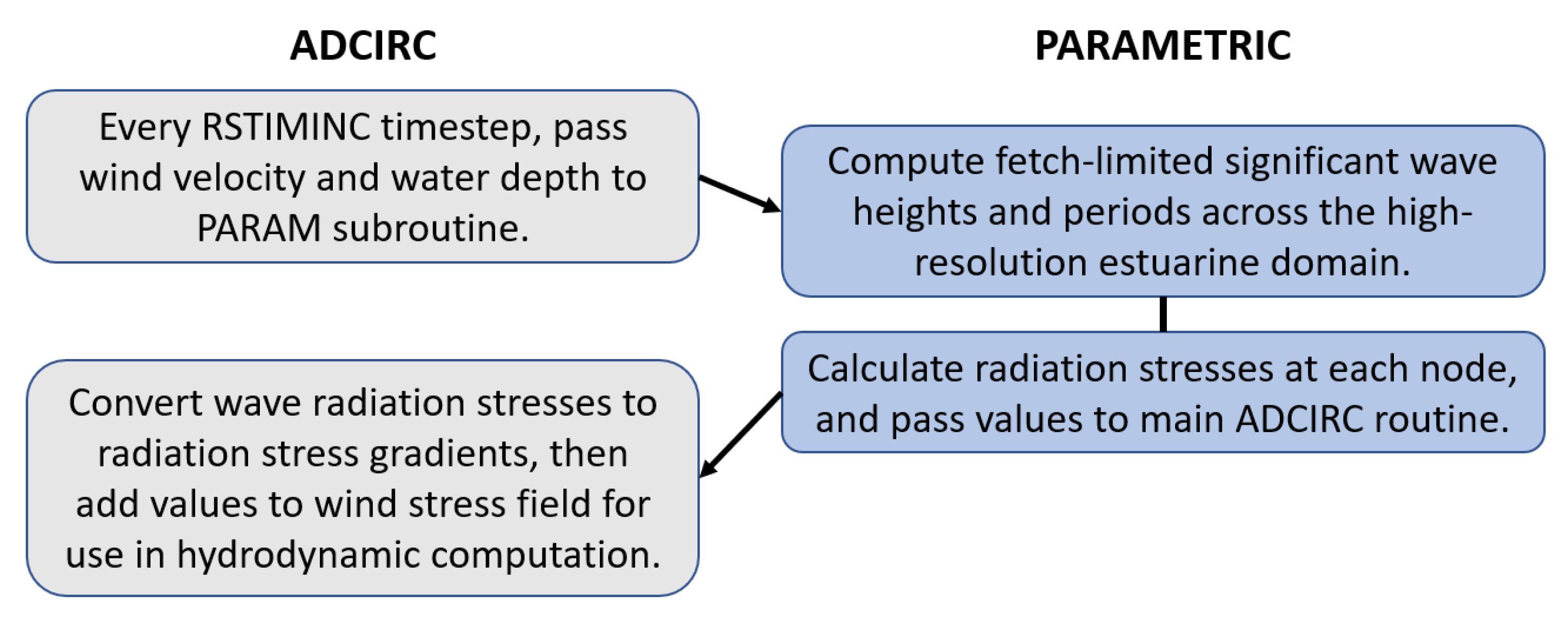
2.1. Parametric Wave Solver
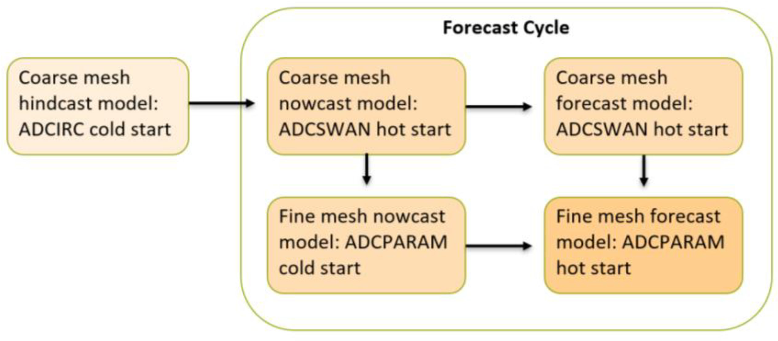
2.2. Multistage Mini-Ensemble Modeling System (MMEMS)
3. Methodology
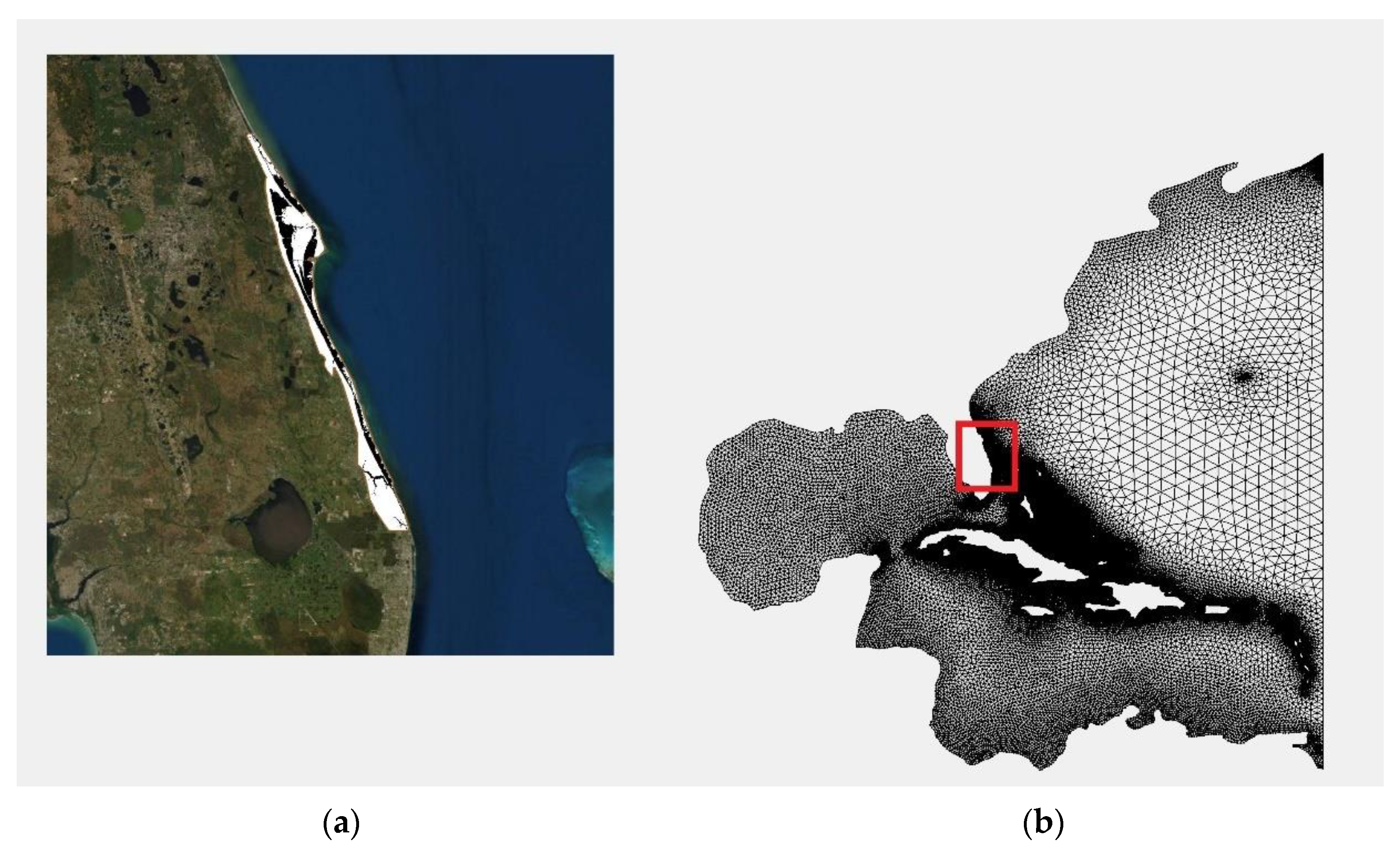
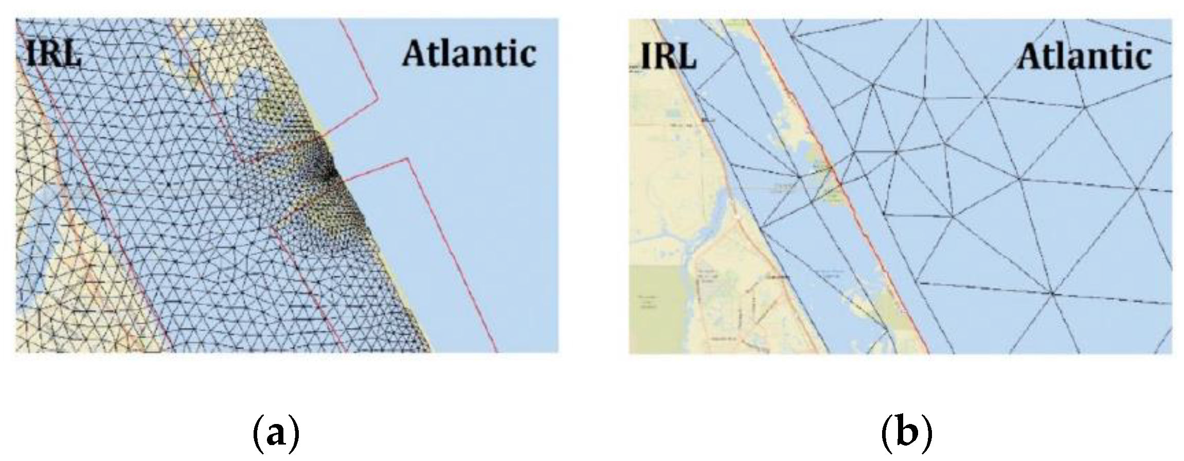
3.1. Model Setup
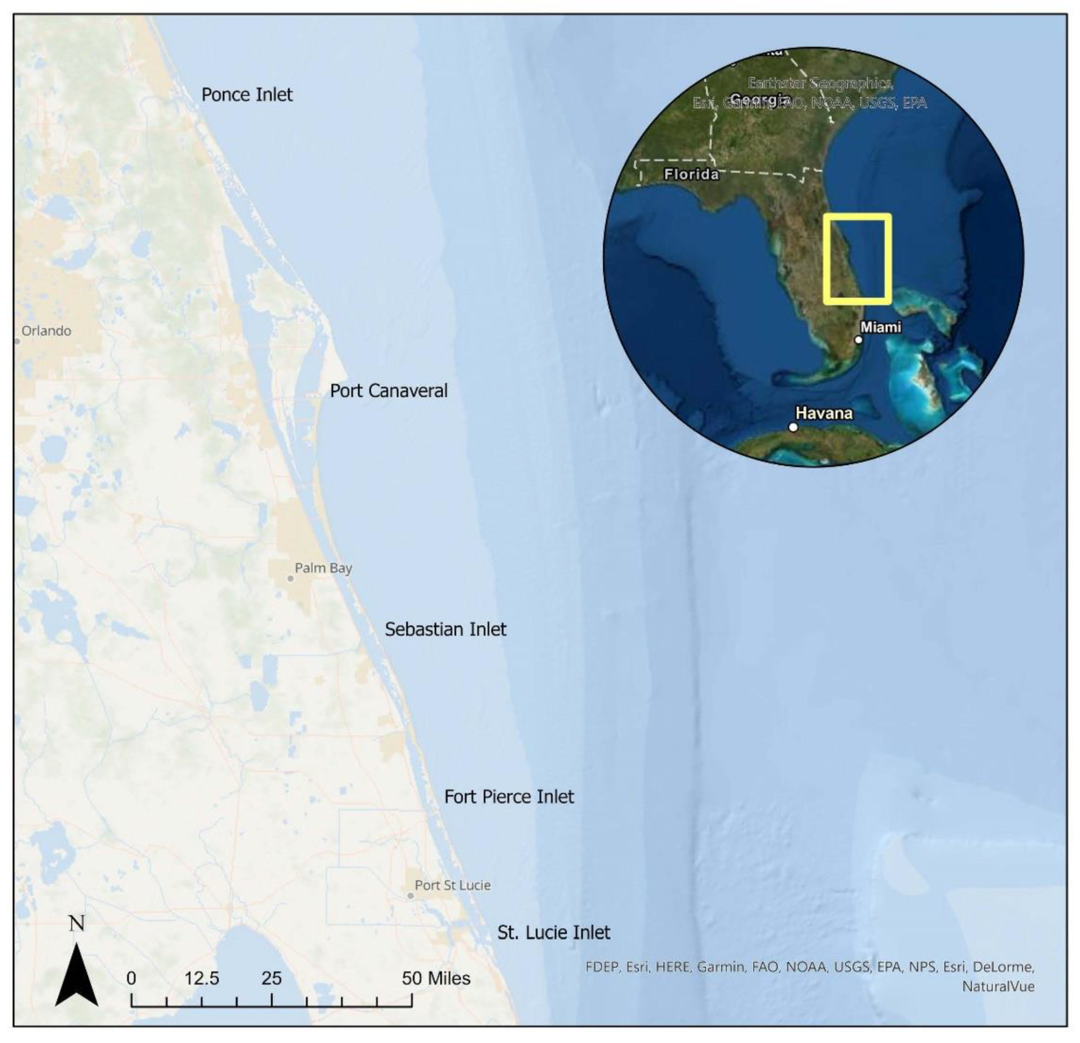
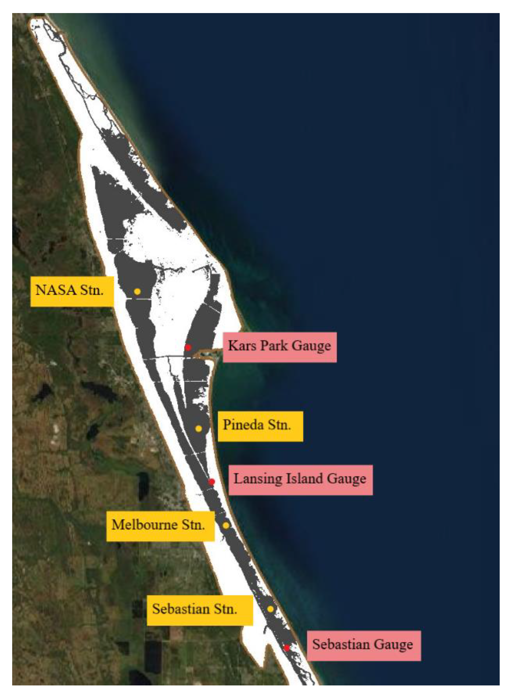
3.2. In-Situ Measurements
4. Results
4.1. Model Runtime
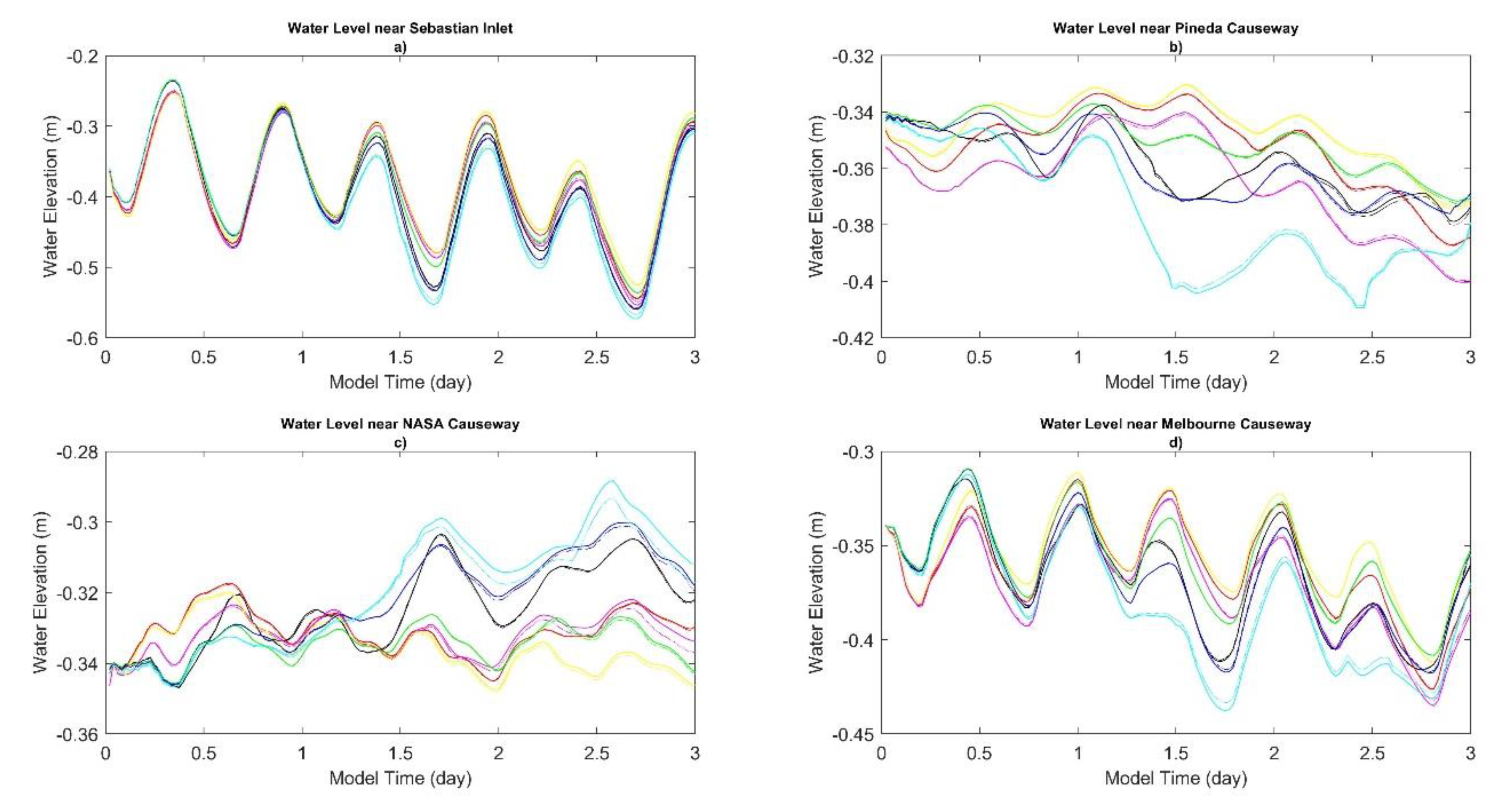
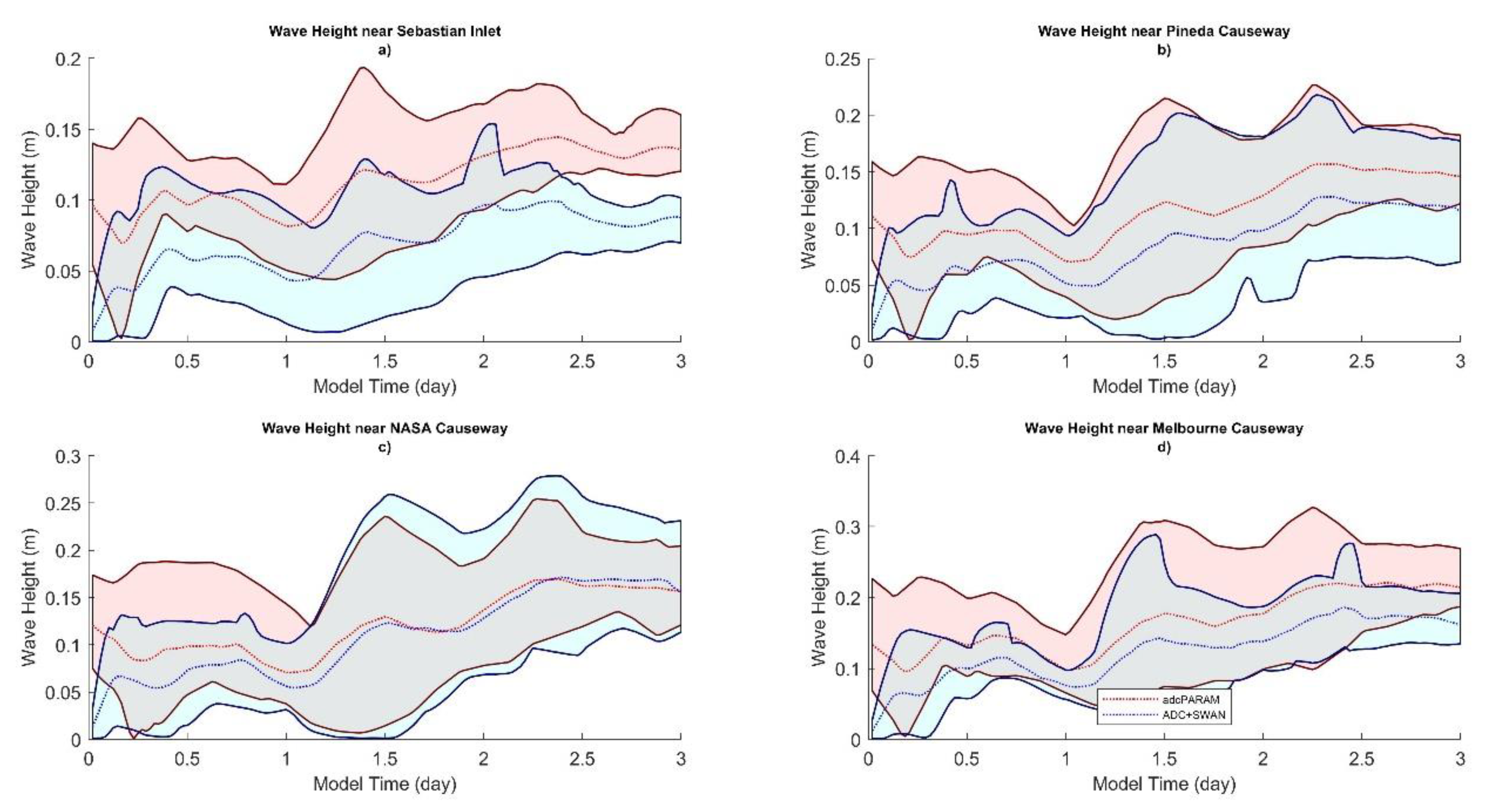
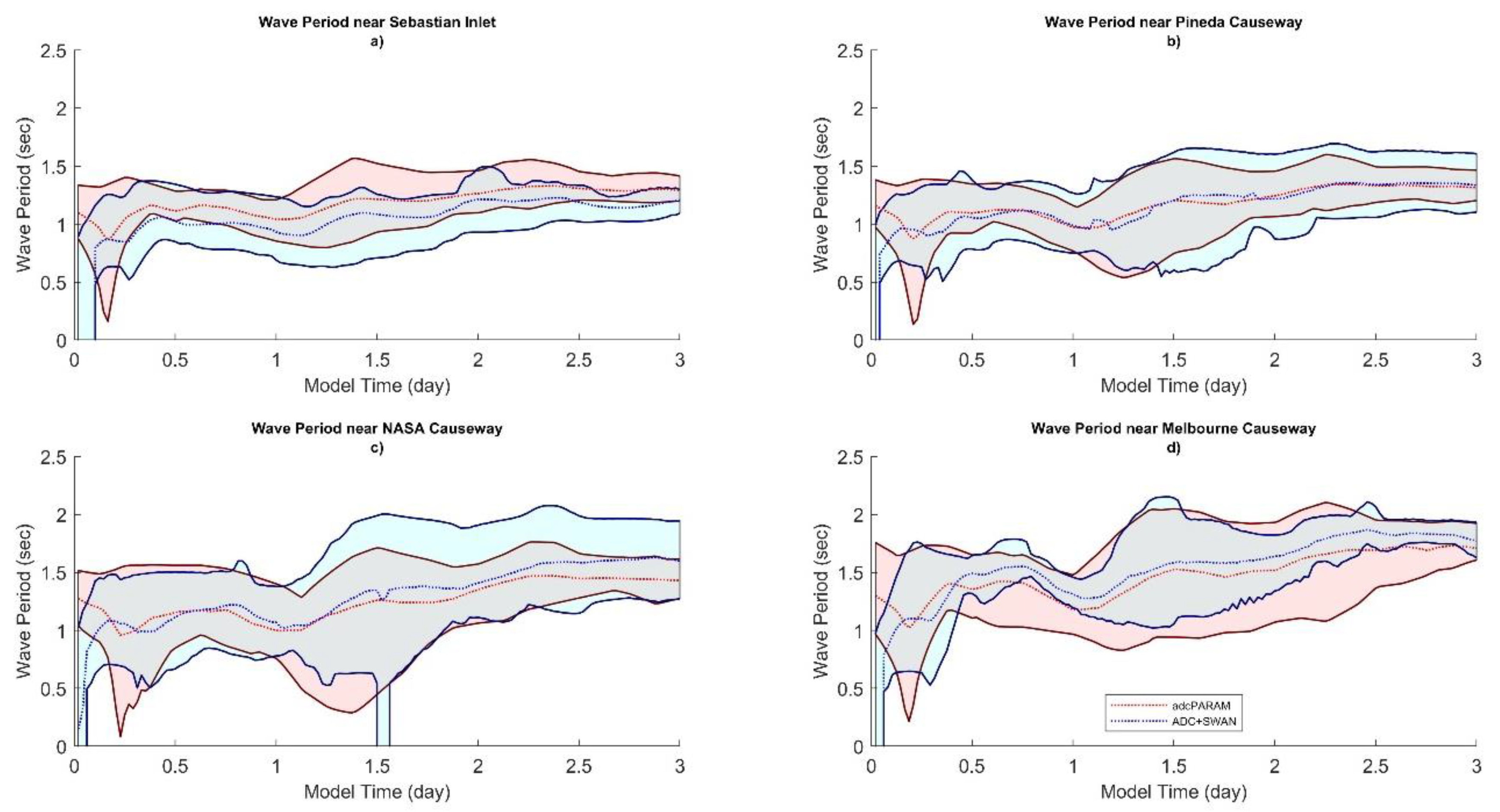
4.2. Model Output
5. Discussion
6. Conclusions
Author Contributions
Funding
Institutional Review Board Statement
Informed Consent Statement
Data Availability Statement
Conflicts of Interest
Appendix A


References
- Roelvink, J.A.; Reniers, A.J.H.M. A Guide to Modeling Coastal Morphology; World Scientific: Singapore, 2011. [Google Scholar]
- Hoffmann, K.A. Computational Fluid Dynamics; Engineering Education System: Wichita, KS, USA, 2004. [Google Scholar]
- Bender, M.A.; Knutson, T.R.; Tuleya, R.E.; Sirutis, J.J.; Vecchi, G.A.; Garner, S.T.; Held, I.M. Modeled Impact of Anthropogenic Warming on the Frequency of Intense Atlantic Hurricanes. Science 2010, 327, 454–458. [Google Scholar] [CrossRef] [PubMed]
- Knauss, J.A.; Garfield, N. Introduction to Physical Oceanography; Waveland Press: Long Grove, IL, USA, 2017. [Google Scholar]
- Ardhuin, F.; Alejandro, O. Wind Waves. New Front. Oper. Oceanogr. 2018, 393–422. [Google Scholar]
- CERC. Shore Protection Manual; Department of the Army, U.S. Army Corps of Engineers: Washington, DC, USA, 1984. [Google Scholar]
- Munk, W.H. Origin And Generation Of Waves. Coast. Eng. Proc. 1950, 1, 1. [Google Scholar] [CrossRef]
- Oh, J.-E.; Jeong, W.-M.; Chang, Y.S.; Oh, S.-H. On the Separation Period Discriminating Gravity and Infragravity Waves off Gyeongpo Beach, Korea. J. Mar. Sci. Eng. 2020, 8, 167. [Google Scholar] [CrossRef]
- Weaver, R.; Slinn, D.N.; Smith, J.M. Effect of Wave Forcing on Storm Surge. Coast. Eng. 2005, 4, 1532–1538. [Google Scholar] [CrossRef]
- Lesnik, J.R. Wave Setup on a Sloping Beach; U.S. Army Coastal Engineering Research Center: Springfield, VA, USA, 1977; p. 77. [Google Scholar]
- Luettich, R.A.; Westerink, J.J.; Scheffner, N.W. ADCIRC: An Advanced Three-Dimensional Circulation Model for Shelves, Coasts, and Estuaries, Report 1: Theory and Methodology of ADCIRC-2DDI and ADCIRC-3DL; Coastal Engineering Research Center Department of the Army Waterways Experiment Station, Corps of Engineers: Vicksburg, Mississippi, 1992. [Google Scholar]
- Roelvink, J.A.; Van Banning, G.K.F.M. Design and development of DELFT3D and application to coastal mor-phodynamics. Oceanogr. Lit. Rev. 1995, 11, 925. [Google Scholar]
- Glahn, B.; Taylor, A.; Kurkowski, N.; Shaffer, W.A. The role of the SLOSH model in National Weather Service storm surge forecasting. Natl. Weather Dig. 2009, 33, 3–14. [Google Scholar]
- Reed, C.W.; Brown, M.E.; Sánchez, A.; Wu, W.; Buttolph, A.M. The Coastal Modeling System Flow Model (CMS-Flow): Past and Present. J. Coast. Res. 2011, 59, 1–6. [Google Scholar] [CrossRef]
- Chen, C.; Liu, H.; Beardsley, R.C. An unstructured grid, finite-volume, three-dimensional, primitive equations ocean model: Application to coastal ocean and estuaries. J. Atmos. Ocean. Technol. 2003, 20, 159–186. [Google Scholar] [CrossRef]
- Shchepetkin, A.F.; McWilliams, J.C. The regional oceanic modeling system (ROMS): A split-explicit, free-surface, topography-following-coordinate oceanic model. Ocean Model. 2005, 9, 347–404. [Google Scholar] [CrossRef]
- Sheng, Y.P. Evolution of a Three-Dimensional Curvilinear-Grid Hydrodynamic Model for Estuaries, Lakes and Coastal Waters: CH3D. In Estuarine and Coastal Modeling; ASCE: Reston, VA, USA, 1990; pp. 40–49. [Google Scholar]
- Sheng, Y.P.; Davis, J.R.; Figueiredo, R.; Liu, B.; Liu, H.; Luettich, R.; Paramygin, V.A.; Weaver, R.; Weisberg, R.; Xie, L.; et al. A Regional Testbed for Storm Surge and Coastal Inundation Models—An Overview. Estuar. Coast. Model. 2013, 2011, 476–495. [Google Scholar] [CrossRef]
- Dietrich, J.C.; Tanaka, S.; Westerink, J.J.; Dawson, C.N.; Luettich, R.A., Jr.; Zijlema, M.; Holthuijsen, L.H.; Smith, J.M.; Westerink, L.G.; Westerink, H.J. Performance of the Unstructured-Mesh, SWAN + ADCIRC Model in Computing Hurricane Waves and Surge. J. Sci. Comput. 2012, 52, 468–497. [Google Scholar] [CrossRef]
- Longuet-Higgins, M.; Stewart, R. Radiation stresses in water waves; a physical discussion, with applications. Deep Sea Res. Oceanogr. Abstr. 1964, 11, 529–562. [Google Scholar] [CrossRef]
- Booij, N.; Ris, R.C.; Holthuijsen, L.H. A third-generation wave model for coastal regions: 1. Model description and validation. J. Geophys. Res. Ocean. 1999, 104, 7649–7666. [Google Scholar] [CrossRef]
- Hoque, A.; Perrie, W.; Solomon, S.M. Application of SWAN model for storm generated wave simulation in the Canadian Beaufort Sea. J. Ocean Eng. Sci. 2020, 5, 19–34. [Google Scholar] [CrossRef]
- Massel, S.R. Ocean Surface Waves: Their Physics and Prediction; World Scientific: Singapore, 1996; Volume 11. [Google Scholar]
- Komen, G.J.; Hasselmann, K. On the Existence of a Fully Developed Wind-Sea Spectrum. J. Phys. Oceanogr. 1984, 14, 1271–1285. [Google Scholar] [CrossRef]
- Hasselmann, S.; Hasselmann, K.; Allender, J.H.; Barnett, T.P. Computations and parameterization of the nonlinear energy transfer in a gravity-wave spectrum. Part II: Parameterization of the nonlinear energy transfer for application in wave models. J. Phys. Oceanogr. 1985, 15, 1378–1391. [Google Scholar] [CrossRef]
- Gonçalves, M.; Rusu, E.; Soares, C. Assessment of wind and wave simulations for an enclosed sea using satellite data. In Maritime Engineering and Technology; CRC Press: Boca Raton, FL, USA, 2012. [Google Scholar] [CrossRef]
- Massey, T.C.; Anderson, M.E.; Smith, J.M.; Gomez, J.M.; Jones, R. STWAVE: Steady-State Spectral Wave Model User’s Manual for STWAVE, Version 6.0; Coastal and Hydraulics Laboratory U.S. Army Engineer Research and Development Center: Vicksburg, MS, USA, 2011. [Google Scholar]
- Taeb, P.; Weaver, R.J. An operational coastal forecasting tool for performing ensemble modeling. Estuar. Coast. Shelf Sci. 2019, 217, 237–249. [Google Scholar] [CrossRef]
- Tolman, H.L. A third-generation model for wind waves on slowly varying, unsteady, and inhomogeneous depths and currents. J. Phys. Oceanogr. 1991, 21, 782–797. [Google Scholar] [CrossRef]
- Bretschneider, C.L. Revised Wave Forecasting Relationships. Coast. Eng. Proc. 1951, 1, 1. [Google Scholar] [CrossRef]
- Bretschneider, C.L. Modification of Wave Spectra on The Continental Shelf and in the Surf Zone. Coast. Eng. Proc. 1962, 1, 2. [Google Scholar] [CrossRef]
- U.S. Army Corps of Engineers. Coastal Engineering Manual; U.S. Army Corps of Engineers: Washington, DC, USA, 2002. [Google Scholar]
- Malhotra, A.; Fonseca, M.S. WEMo (Wave Exposure Model): Formulation, Procedures and Validation; NOAA Technocal Memorandum/NOS/NCCOS: Silver Spring, MD, USA, 2007. [Google Scholar]
- Hughes, S.A. TMA Shallow-Water Spectrum: Description and Application, Technical Report; CERC (US Army Engineer Waterways Experiment Station Coastal Engineering Research): Vicksburg, MS, USA, 1984. [Google Scholar]
- Boyd, S.C.; Weaver, R.J. Replacing a third-generation wave model with a fetch based parametric solver in coastal estuaries. Estuar. Coast. Shelf Sci. 2021, 251, 107192. [Google Scholar] [CrossRef]
- Dean, R.G.; Dalrymple, R.A. Water Wave Mechanics for Engineers and Scientists; World Scientific: Singapore, 1992; Volume 2. [Google Scholar]
- Putnam, J.A.; Johson, J.W. The dissipation of wave energy by bottom friction. Trans. Am. Geophys. Union 1949, 30, 67–74. [Google Scholar] [CrossRef]
- Holthuijsen, L.H.; Booji, N.; Haagsma, J.G.; Kieftenburg, A.T.M.M.; Ris, R.C.; van der Westhuysen, A.J.; Zijlema, M. SWAN Cycle III Version 40.41 User’s Manual; Delft University of Technology Press: Delft, The Netherlands, 2004. [Google Scholar]
- Mukai, A.Y.; Westerink, J.J.; Luettich, R.A., Jr.; Mark, D. Eastcoast 2001, a Tidal Constituent Database for Western North Atlantic, Gulf of Mexico, and Caribbean Sea; US Army Corps of Engineers Engineer Research and Development Center: Vicksburg, MS, USA, 2002. [Google Scholar]
- Fleming, J.G.; Fulcher, C.W.; Luettich, R.A.; Estrade, B.D.; Allen, G.D.; Winer, H.S. A Real Time Storm Surge Forecasting System Using ADCIRC. In Estuarine and Coastal Modeling; American Society of Civil Engineers: Reston, VA, USA, 2008; pp. 893–912. [Google Scholar]
- Dietrich, J.C.; Dawson, C.N.; Proft, J.M.; Howard, M.T.; Wells, G.; Fleming, J.G.; Luettich, R.A.; Westerink, J.J.; Cobell, Z.; Vitse, M.; et al. Real-Time Forecasting and Visualization of Hurricane Waves and Storm Surge Using SWAN + ADCIRC and FigureGen. In Computational Challenges in the Geosciences; Springer: New York, NY, USA, 2013; pp. 49–70. [Google Scholar] [CrossRef]
- Rogers, E.; DiMego, G.; Black, T.; Ek, M.; Ferrier, B.; Gayno, G.; Janjic, Z.; Lin, Y.; Pyle, M.; Wong, V.; et al. The NCEP North American mesoscale modeling system: Recent changes and future plans. In Proceedings of the 23rd Conference on Weather Analysis and Forecasting/19th Conference on Numerical Weather Prediction, Omaha, NE, USA; 2009. [Google Scholar]
- Toth, Z.; Kalnay, E. Ensemble Forecasting at NCEP and the Breeding Method. Mon. Weather Rev. 1997, 125, 3297–3319. [Google Scholar] [CrossRef]
- McQueen, J.; Du, J.; Zhou, B.; DiMego, G.; Juang, H.; Ferrier, B.; Manikin, G.; Rogers, E.; Black, T.; Toth, Z. Overview of the NOAA/NWS/NCEP Short Range Ensemble Forecast (SREF) System; NOAA NWS: Silver Spring, MD, USA, 2004. [Google Scholar]
- Luettich, R.A.; Westerink, J.J. Implementation of the Wave Radiation Stress Gradient as a Forcing for the ADCIRC Hydrodynamic Model: Upgrades and Documentation for ADCIRC Version 34.12; Coastal Engineering Research Center Department of the Army Waterways Experiment Station, Corps of Engineers: Vicksburg, MS, USA, 1999. [Google Scholar]
- National Hurricane Center. 2021 Tropical Cyclone Advisory Archive. 2021. Available online: https://www.nhc.noaa.gov/archive/2021/ (accessed on 8 August 2022).
- Onset Computer Corporation. Hobo and StowAway Data Loggers. 2021. Available online: http://www.onsetcomp.com (accessed on 8 August 2022).
- Aquaveo. SMS User Manual (v11.1) Surface-Water Modeling System. 2013. Available online: https://www.aquaveo.com/software/sms-surface-water-modeling-system-introduction (accessed on 8 August 2022).
- Weaver, R.J.; Taeb, P.; Lazarus, S.; Splitt, M.; Holman, B.P.; Colvin, J. Sensitivity of modeled estuarine circulation to spatial and temporal resolution of input meteorological forcing of a cold frontal passage. Estuar. Coast. Shelf Sci. 2016, 183, 28–40. [Google Scholar] [CrossRef]
- Hasselmann, K.; Barnett, T.P.; Bouws, E.; Carlson, H.; Cartwright, D.E.; Enke, K.; Ewing, J.A.; Gienapp, A.; Hasselmann, D.E.; Kruseman, P.; et al. Measurements of Wind-Wave Growth and Swell Decay during the Joint North Sea Wave Project (JONSWAP); Deutsches Hydrographisches Institut: Hamburg, Germany, 1973. [Google Scholar]
- Mitsuyasu, H.; Tasai, F.; Suhara, T.; Mizuno, S.; Ohkusu, M.; Honda, T.; Rikiishi, K. Observation of the Power Spectrum of Ocean Waves Using a Cloverleaf Buoy. J. Phys. Oceanogr. 1980, 10, 286–296. [Google Scholar] [CrossRef]
- Reid, R.O.; Bretschneider, C.L. Surface Waves and Offshore Structures: The Design Wave in Deep or Shallow Water, Storm Tide, and Forces on Vertical Piles and Large Submerged Objects: A Technical Report. 10. A. & M; College of Texas: Tyler, TX, USA, 1953. [Google Scholar]


| Estuarine Model | Average Wall Time (min) |
|---|---|
| ADCIRC + SWAN | 180 |
| ADCIRC + PARAM | 88 |
| Model | Overall Wall Time (min) |
|---|---|
| ADCIRC + SWAN MMEMS | 2176 |
| ADCIRC + PARAM MMEMS | 1443 |
| Bias | NMAE | |
|---|---|---|
| Water Elevation (mm) | −0.189 | 0.23% |
| Wave Height (m) | −0.0303 | 51.53% |
| Wave Period (s) | 0.0631 | 10.44% |
Publisher’s Note: MDPI stays neutral with regard to jurisdictional claims in published maps and institutional affiliations. |
© 2022 by the authors. Licensee MDPI, Basel, Switzerland. This article is an open access article distributed under the terms and conditions of the Creative Commons Attribution (CC BY) license (https://creativecommons.org/licenses/by/4.0/).
Share and Cite
Lodge, C.T.; Weaver, R.J. Coupling a Parametric Wave Solver into a Hydrodynamic Circulation Model to Improve Efficiency of Nested Estuarine Storm Surge Predictions. J. Mar. Sci. Eng. 2022, 10, 1117. https://doi.org/10.3390/jmse10081117
Lodge CT, Weaver RJ. Coupling a Parametric Wave Solver into a Hydrodynamic Circulation Model to Improve Efficiency of Nested Estuarine Storm Surge Predictions. Journal of Marine Science and Engineering. 2022; 10(8):1117. https://doi.org/10.3390/jmse10081117
Chicago/Turabian StyleLodge, Caleb T., and Robert J. Weaver. 2022. "Coupling a Parametric Wave Solver into a Hydrodynamic Circulation Model to Improve Efficiency of Nested Estuarine Storm Surge Predictions" Journal of Marine Science and Engineering 10, no. 8: 1117. https://doi.org/10.3390/jmse10081117
APA StyleLodge, C. T., & Weaver, R. J. (2022). Coupling a Parametric Wave Solver into a Hydrodynamic Circulation Model to Improve Efficiency of Nested Estuarine Storm Surge Predictions. Journal of Marine Science and Engineering, 10(8), 1117. https://doi.org/10.3390/jmse10081117