Abstract
This manuscript describes methods for evaluating the efficacy of five satellite-based Chlorophyll-a algorithms in Chesapeake Bay, spanning three separate sensors: Ocean Land Color Imager (OLCI), Visible Infrared Imaging Radiometer Suite (VIIRS), and MODerate Resolution Imaging Spectroradiometer (MODIS). The algorithms were compared using in situ Chlorophyll-a measurements from 38 separate stations, provided through the Chesapeake Bay Program (CBP). These stations span nearly the entire 300 km length of the optically complex Chesapeake Bay, the largest estuary in the United States. Overall accuracy was examined for the entire dataset, in addition to assessing the differences related to the distance from the turbidity maximum to the north by grouping the results into the upper bay, middle bay, or lower bay. The mean bias and the Mean Absolute Error (MAE) as well as the median bias and Median Absolute Error (MedAE) were conducted for comparison. A two-band algorithm, that is based on the red-edge portion of the electromagnetic spectrum (RE10), when applied to OLCI imagery, exhibited the lowest overall MedAE of 36% at all stations. As a result, it is recommended that the RE10 algorithm be applied to OLCI and provided as an operational product through NOAA’s CoastWatch program. The paper will conclude with results from a brief climatological analysis using the OLCI RE10 algorithm.
1. Introduction
Chlorophyll-a (chla) is the dominant photosynthetic pigment within the phytoplankton community, which is the base of the marine food-web. By determining the concentration of chla, a reasonable approximation of overall biomass can be achieved. From this point, various modeling approaches have been undertaken to estimate primary production both in Chesapeake Bay [1] and elsewhere [2]. Chla is also an important parameter for modeling various other biophysical factors such as the size of hypoxic zones, areas that can support submerged aquatic vegetation (SAV), and to set total maximum daily load (TMDL) thresholds [3,4,5]. Furthermore, chla concentrations can also be used to determine site selection for aquaculture facilities [6]. Remote sensing, and specifically satellite-derived remote sensing, provides an effective synoptic approach to measuring the chla biomass within a system, which in turn can be used as a proxy for eutrophication. As chla is a critical component to assessing water quality within a system, high temporal frequency and spatial resolution satellite chla could provide more information than traditional field sampling to assess ecological and management implications [7]. There have been tremendous efforts towards algorithmic development for accurate coastal chla using satellite-based ocean color sensors. These ocean color sensors started in the 1970s with the Coastal Zone Color Scanner (CZCS), continued into the 1990s with the Sea-viewing Wide Field-of-view Sensor (SeaWiFS), then into the 2000s with Moderate Resolution Imaging Spectroradiometer (MODIS) and Medium Resolution Imaging Spectrometer (MERIS), and into the 2010s with the Visible Infrared Imaging Radiometer Suite (VIIRS) and the Ocean Land Color Imager (OLCI), among others.
Aquatic environments are characterized into two main categories based on their optical properties: Case 1 and Case 2 waters [8]. Case 1 waters are defined as waters where the optical properties are dominated by phytoplankton and their degradation products, while Case 2 waters are defined as waters where the optical properties are also influenced by other materials. In general, Case 1 waters are found offshore and standard chla algorithms reliably estimate the chla concentration. However, chla concentrations are not as easily estimated in Case 2 waters, primarily due to the confounding effects from colored dissolved organic matter (CDOM) and from total suspended sediments (TSS) and their associated pigments. In this paper we will discuss the performance of five algorithms, spanning three separate sensors, in determining the chla concentrations in the Case 2 waters of Chesapeake Bay located on the east coast of North America. The paper will layout a framework to determine the efficacy of evaluating algorithms with coincident field data in an effort to deliver the best-quality algorithm to a national satellite observing system.
1.1. Algorithms
Perhaps the most widely used global ocean color chla algorithms are a suite of biophysically based blue/green ratio algorithms known as the Ocean Color (OCx) algorithms. OCx includes the OC2, OC3, and OC4 algorithms, among others, which use either two, three, or four bands respectively, with one band in the green portion of the electromagnetic spectrum and the remaining bands in the blue portion. They are based on a ratio of the reflectance of blue light to green light, which in turn is based on the fact that chla and associated carotenoid pigments strongly absorb blue light in the electromagnetic spectrum, but not green light. The OC3 and OC4 algorithms are so-called band switching algorithms, which use multiple blue bands, switching to longer wavelengths as the absorption increases. These algorithms were primarily developed for Case 1 waters where phytoplankton and their degradation products dominate the optics of the water [8,9]. In Case 1 waters, the largest difference in absorption of chla occurs between the blue bands (highest chla absorption) and the green band (location of the lowest chla absorption), and therefore the higher the difference in the blue and green remote sensing reflectance (Rrs) peaks, the higher the chla concentration and thus the more phytoplankton that are in the water. These algorithms are generally most critical in clear waters where chla concentrations and signal-to-noise ratios will be lowest. OCx algorithms using additional bands are currently being developed for the newer generation of hyperspectral sensors such as the Plankton, Aerosol, Cloud ocean Ecosystem sensor [10].
Here, we will test the efficacy of four different OCx algorithms. The first to be considered is the OC4 algorithm from the OLCI sensor. The next three OCx algorithms to be tested are operationally produced by the National Oceanic and Atmospheric Administration’s CoastWatch program [11]. The first of the CoastWatch suite of algorithms is the MODIS-Wang algorithm, which is based on OC3 spectrally adjusted for the MODIS bands [12]. The next is the MODIS-Werdell algorithm developed by Werdell et al. (2009) [13], which is based on the OC3 algorithm from MODIS, and was regionally tuned for improved retrieval of chla concentrations in Chesapeake Bay. The final OCx algorithm to be considered is the VIIRS-SciQual algorithm of Wang et al. (2017) [14], which is based on OC3, adjusting the algorithm for the VIIRS spectral bands.
There have been various algorithms that were developed for Case 2 waters. Generally, Case 2 chla algorithms use bands located at or near the red area of the electromagnetic spectrum (so called “red-edge” algorithms). Chla has two absorption peaks, with the primary absorption peak located in the blue region of the spectrum, with a large absorption dip in the green region, followed by a smaller secondary absorption peak in the red portion of the spectrum [15]. There are advantages and disadvantages to using these algorithms as opposed to the OCx suite of algorithms. CDOM and detrital pigments (those associated with non-algal particles) absorb blue light strongly. Case 2 water is typically high in CDOM and TSS and as such will overestimate chla when high concentrations of these materials are present. Case 1 waters typically have extremely low levels of CDOM, TSS, or particulate organic material (POM), and this potential overestimation is not an issue. However, red and near-infrared (NIR) bands strongly absorb water. At a wavelength of 665 nm, less than 10% of the light in pure water originates from deeper than 2.5 m [16]. Adding additional light-absorbing material into the water (phytoplankton, CDOM, TSS, etc.) will only shoal the optical depth. As a result, chla present deeper than 2.5 m will provide only a small portion of the signal in algorithms that utilize red bands. One such algorithm that uses the red-edge band is the aforementioned Red Edge 2010 (RE10) algorithm [17]. The efficacy of the RE10 algorithm and the previously described four OCx-based algorithms will be tested on their abilities to estimate in situ chla data provided by the CBP [18].
1.2. Study Area
Chesapeake Bay (Figure 1) is the largest estuary in the United States and one of the largest estuaries in the world. It is a classic example of a drowned river valley type of estuary, with approximately half of the freshwater component coming from the Susquehanna River, at the head of the bay. There are a number of other smaller rivers that flow into Chesapeake Bay, including the Potomac (providing ~18% of freshwater flow) and the James River (providing ~14% of freshwater flow) [19]. The bay is approximately 300 km long and 4.5 km at its narrowest point and 50 km at its widest point. The mean depth of the bay is 7 m, with ~24% being less than 2 m deep. There is a deep channel down the center, with wide shallow shoals on either side of the channel. The Chesapeake Bay lies within the US states of Maryland and Virginia, but the massive 166,000 km2 watershed extends into four additional states (Delaware, West Virginia, Pennsylvania, and New York) and the District of Columbia. The bay has experienced drastic eutrophication in the last 100 years caused primarily by increased anthropogenic pressures [20]. This eutrophication has been exacerbated by the 99% loss of the eastern oyster, Crassostrea virginica, a keystone species which effectively filters water, thereby reducing chla concentrations as well as optical complexity [21].
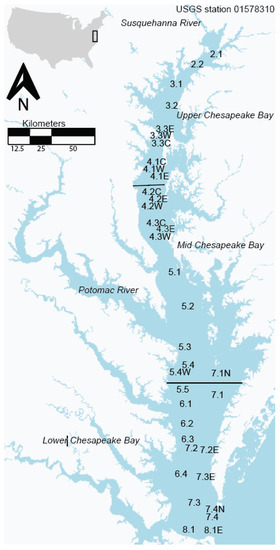
Figure 1.
Map of the study area, showing each monitoring station from the Chesapeake Bay Program used in this study. The map is based on a 300-m OLCI image, the same spatial resolution used from the RE10 algorithm.
2. Materials and Methods
2.1. Field Methods
Field data were acquired from the CBP. Chla and pheophytin were determined using acetone extraction from a ground filter and then the chla was calculated from readings of optical density at several wavelengths using a spectrophotometer [18].
2.2. Satellite Sensors
Imagery from three different sensors onboard several different spacecrafts was examined in this analysis. Daily OLCI images collected onboard the Copernicus Sentinel-3A and 3B satellite data from the European Organization for the Exploitation of Meteorological Satellites (EUMETSAT) were processed by NOAA’s National Centers for Coastal Ocean Science. Daily OLCI imagery was processed at its native resolution (300 m pixel) and additional processing (including invalid pixel flags) was conducted as outlined by Wolny et al. [22] for Chesapeake Bay and described in Wynne et al. [23]. The map in Figure 1 provides a sense of the spatial resolution of the OLCI sensor. The OLCI sensor operates on two separate spacecraft: Sentinel-3A (launched February 2016) and Sentinel-3B (launched April 2018). There are plans to launch OLCI sensors on two other spacecraft: Sentinel-3C (projected 2024 launch) and Sentinel-3D (projected 2028 launch). Daily imagery from both Sentinel-3A and Sentinel-3B from April 2016 through April 2021 was used in this study.
Chla derived from OLCI was compared with operational Visible Infrared Radiometer Suite (VIIRS) products, collected onboard the Suomi spacecraft daily at a native resolution of 700 m. These data were provided by NOAA’s CoastWatch program for the period of June 2016–December 2019. An additional comparison was made with operational chla products from the Moderate Resolution Imaging Spectroradiometer (MODIS), which were collected daily onboard the Aqua spacecraft, processed with a native resolution of 1000 m, and provided by CoastWatch for the same period.
2.3. Chla Algorithms
Five separate algorithms were examined for accuracy. Each algorithm will be presented along with field data matchups from the CBP. The first two algorithms were applied to OLCI data and will be referred to as the RE10 algorithm [17] and the OLCI-OC4 algorithm [9], respectively. The OLCI-OC4 algorithm was retrieved from remote sensing reflectances (Rrs) obtained from l2gen in SeaDAS (NASA REF). RE10 was calculated with dimensionless water reflectances using an assumption of coarse-mode maritime aerosol, with dark water at 885 nm, spectrally flat f/Q, and applying them to a bio-optical ratio algorithm that provides compensation for residual errors [24] (Stumpf and Pennock, 1989). This atmospheric correction method is applied because it retrieves more pixels, especially in tributaries, within Chesapeake Bay. Ioannou et al. (2014) [25] noted that a significant issue with utilizing algorithms that use NIR bands is related to imperfect atmospheric corrections. However, a ratio algorithm has relatively small residual aerosol error, particularly with bands that are relatively close, such as 665 nm and 709 nm [26]. On the other hand, because the OLCI-OC4 algorithm uses blue bands, it requires variable aerosol models, necessitating the l2gen SeaDAS atmospheric corrections.
Gilerson et al. (2010) [17] derived two separate but related chla algorithms, a 2-band algorithm and a 3-band algorithm, but subsequent work [27,28] indicated that the simpler 2-band algorithm performs as well or better. We implement a modified version of Gilerson et al. (2010) [17] applied to OLCI where:
Taking aw(665) = 0.4245 m−1 and aw(709) = 0.7864 m−1 and p = 0.89, Equation (1) can be rewritten as:
where R2 is the ratio of dimensionless water reflectance where the red band, λ1 = 665 nm, and the NIR band, λ2 = 709 nm, are atmospherically corrected with an assumption of a coarse-mode maritime aerosol, with dark water at 885 nm such that:
where is the top-of-atmosphere (TOA) reflectance. The final chla equation was regionally adjusted by substituting the original offset coefficient of 19.30 in Gilerson et al. (2010) [17] with a new offset coefficient of 14.30 [23], such that:
The OLCI-OC4, or OC4ME, is a Maximum Band Ratio (MBR), polynomial-based semi-analytical algorithm based on Apparent Optical Properties (AOP) and is expressed in Equation (5):
is the ratio of irradiance–reflectance of band i among the blue bands centered at 443, 490, and 510 nm over that of the green band, j, centered at 560 nm. Ax is the chlorophyll-a and x is the order of the polynomial (e.g., 1st through 4th). The band for the numerator is selected so that the ratio is maximized [29].
The datasets for the additional three algorithms were provided directly from the NOAA CoastWatch program. These data are run operationally: the MODIS images are from the Aqua spacecraft and provided in near-real time, whereas the VIIRS-SciQual images are from the Suomi-NPP spacecraft and delayed by 14 days for science-quality accuracy. The MODIS-Wang algorithm uses a SWIR-NIR atmospheric correction [12]. This atmospheric correction negates the “black-pixel” assumption, that states that water is spectrally black for NIR wavelengths, which is typical of Case 1 waters but is not necessarily true in Case 2 waters [30]. Ideally, the SWIR correction generates more accurate chla retrievals for Case 2 waters than the NIR correction, so the MODIS-Wang approach uses a single OC3 algorithm with a combined SWIR-NIR atmospheric correction that distinguishes between the two water types. The MODIS-Werdell algorithm uses a NIR atmospheric correction but regionally tunes the OC3 algorithm with coefficients calculated from Chesapeake Bay in-situ chla measurements [13]. This regional tuning reduces the high chla bias typical of OC3 retrievals in Case 2 waters. The final algorithm, the VIIRS-SciQual, uses an atmospheric correction developed by [31] Jiang and Wang (2014), which is an iterative NIR approach combining the methods of [32] Bailey et al. (2010), MUMM [33], and Wang et al. [34], referred to as the BMW atmospheric correction. Jiang and Wang [31] found this approach offered more accurate results compared to other NIR approaches. Furthermore, the delayed mode post-processing for science quality introduces additional calibration for the Suomi-NPP VIIRS blue band for increased chla accuracy, among other science quality enhancements [14].
The OLCI satellite data were screened prior to use and a pixel was not used for further analysis unless it retrieved all pixels within a 3 × 3 (900 m) box around the station of interest, and the satellite overpass coincided within ±3 h from the sample collection time [35]. The RE10 is insensitive to chla < 1 µg L−1, so a sample was rejected for the OLCI TOA algorithms unless the chla was > 1 µg L−1 and the Rayleigh-corrected surface reflectance at 885 nm (ρ885) was greater than 0.5 (dimensionless). If a station met these criteria, the median value of the 3 × 3 box was calculated and reported as the satellite-based chla concentration. In addition, all available pixels that met the quality flag were selected at each station and plotted against the field chla to show the stability of the algorithm over time. Again, the median of the nine closest pixels to each of the 38 stations was selected.
For MODIS data, pixels were first gridded to a 1 km spatial resolution Mercator grid on a per-overpass basis, using only the pixel closest to each grid cell’s center location. Gridded overpasses were then combined by grid cell into a daily composite on the same Mercator grid, this time using the pixel with the smallest nadir angle, since there may be at most two spacecraft overpasses per day over Chesapeake Bay. Data were extracted from the daily gridded data for a 3 × 3 grid-cell box (3 km) around each station of interest and median chla was calculated if the 3 × 3 box contained all nine values. Medians for the day of sample collection were used, yielding coincident matchups with the CBP field data within 12 h. For VIIRS, the same procedure was used, except on a 750 m spatial resolution grid for the gridded daily overpasses and daily composites.
The chla image products from OLCI, MODIS, and VIIRS were compared in their native resolutions, as the purpose of this analysis was to demonstrate operational applicability of the imagery. A 3 × 3 pixel box was extracted in all cases to screen for any cloud contamination, glint, or other erroneous pixels, even though this led to a difference in the footprint that is being compared with field data. It was important for this study to compare the operational products as is, with the RE10 products from OLCI to demonstrate their preference for operational use in Chesapeake Bay, given differences in atmospheric correction, spatial resolution, and a shift to the red-NIR wavelengths.
Overall, 38 stations from the CBP were selected, as shown in Figure 1. The stations represent a wide range of values spanning from the head of the bay to the near oceanic waters near the bay mouth, including the estuarine turbidity maximum (ETM) [36].
2.4. Comparative Analysis
The daily spectrophotometric chla from the CBP (henceforth called field chla) was used to determine the efficacy of the remotely sensed chla concentrations derived from the five different algorithms. The only field chla values that were used were surface values. The daily matchups were made for each individual station as well as cumulatively for three specified regions (upper bay, middle bay, and lower bay), as well as all of the stations together to provide a bay-wide result.
2.5. Error Metrics
To determine the accuracy of the individual algorithms, the multiplicative mean bias, the Mean Absolute Error (MAE), the median bias, and the Median Absolute Error (MedAE) were calculated. These metrics were selected following recommendations outlined by Seegers et al. (2018) [37] to evaluate whether the RE10 algorithm performed better in Chesapeake Bay than available operational chla products currently delivered through CoastWatch. These same methods (bias and MAE) were also successfully adapted to OLCI intercalibration techniques by Wynne et al. (2021) [38], using these same ρs values. Both the median and mean absolute errors and biases were chosen in an effort to address how the errors between the algorithms and stations are distributed. The median error captures the typical error, while the mean error will reflect whether a method tends to have outlier errors. Given the screening methods used for the image matchups (Section 2.2), we would assume that these outliers are likely valid data points. The bias (mean bias and median bias) quantifies the systematic error or the difference between the modeled value (M) (in this case, the satellite chla) and the observed or reference value (O) (in this case, the field chla data). As the analysis used log-transformed data, the mean multiplicative bias was determined in Equation (6):
where M is the modeled chla (satellite chla), O is the observed (field chla), and n is the sample size (number of matchups available). The closer the multiplicative bias is to a value of 1, the less algorithmic bias exists, leading to better model accuracy. For example, a bias of 1.2 indicates a model that overestimates by ~20%, and a mean bias of 0.8 indicates a model that underestimates by ~20% (this is approximate). Seegers et al. [37] noted there is not a simple direct match between multiplicative bias and percentage error. A consistent bias (i.e., a bias that is present in the vast majority of modeled-to-observed data pairs) can be easily corrected by introducing a multiplicative correction factor. The median multiplicative bias captures the central tendency of the data, the mean multiplicative bias, if it deviates substantially from the median, captures whether the samples with large errors are unevenly distributed. The MAE captures the error magnitude, highlighting the absolute error between the observed and modeled quantities. The MAE is defined in Equation (7) as:
The MAE equation uses the same variables as the bias equation (Equation (4)). The MAE is multiplicative, therefore, a MAE value of 1.2 indicates that the error is about 0.2 × the observed value (or ~20%). Multiplicative error metrics are most appropriate for distributions that have errors that are proportional to magnitude, such as the case here. The median bias and the Median Absolute Error (MedAE) were calculated in the same fashion as the mean bias and the MAE, except for replacing the mean values with the median values in Equations (4) and (5).
3. Results
3.1. Matchup between RE10 and OC4 Using the Field Data
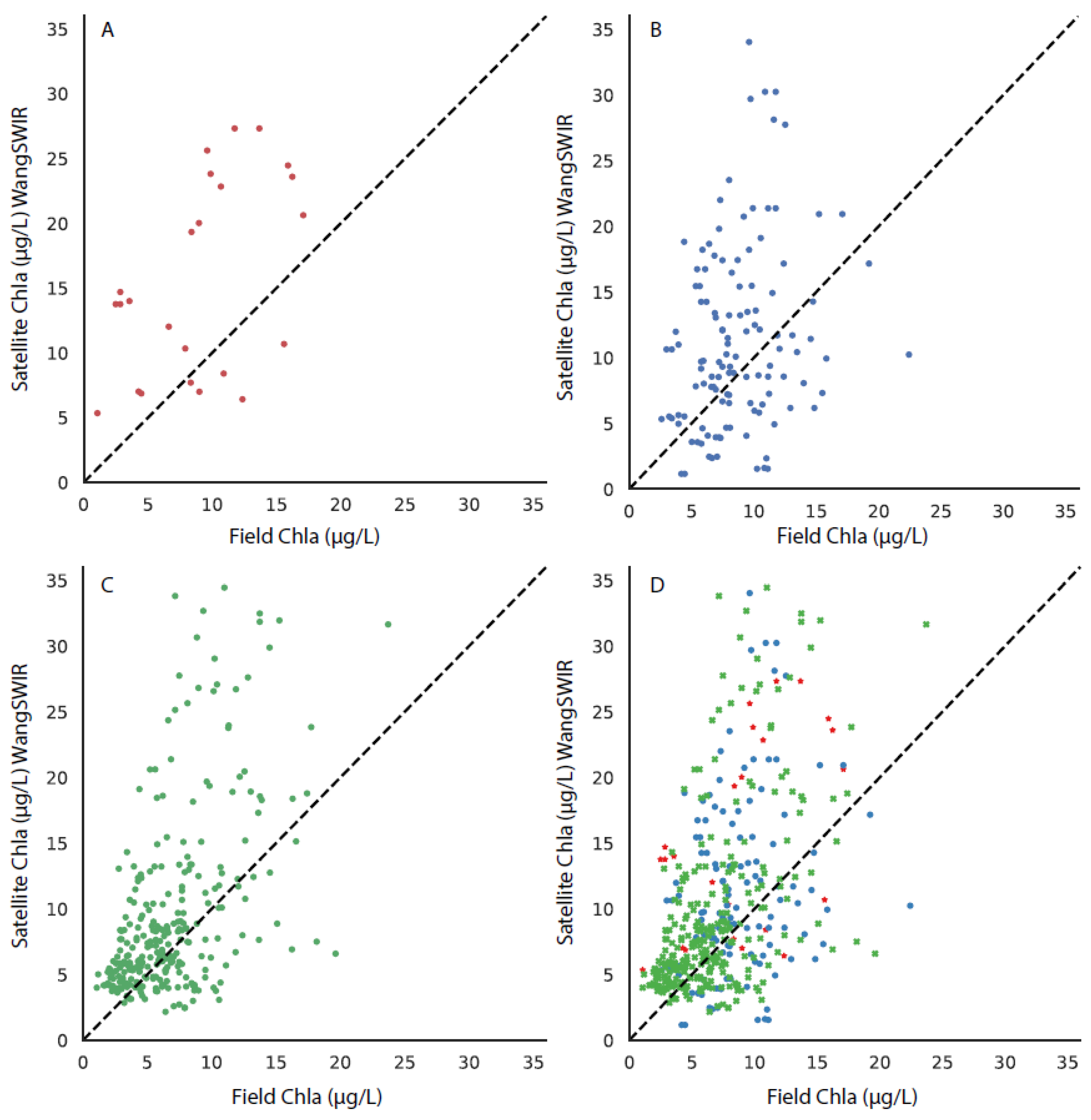
The matchup between the OLCI RE10 chla, OLCI-OC4 chla, and the field chla are shown in Figure 2 and Figure 3. Panel A in both figures shows the relationship with the stations in the upper bay, panel B shows the relationship in the stations in the middle bay, panel C shows the relationship in the lower bay, and panel D shows the relationship with all of the stations. The RE10 algorithm (Figure 2) outperforms the OLCI-OC4 (Figure 3) as there is a more equal distribution around the 1:1 line. There is a tighter 1:1 correlation in the more southerly stations, which is expected given the greater distance from the influence of the Susquehanna River and the ETM to the north.
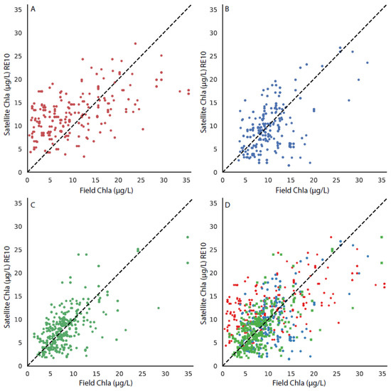
Figure 2.
The matchup between the field chla and the OLCI-RE10 algorithm, with the 1:1 line shown in each subplot for stations in (A) the upper bay, (B) the middle bay, (C) the lower bay, and (D) all stations, with the upper, middle, and lower bays differentiated by symbol color and style.
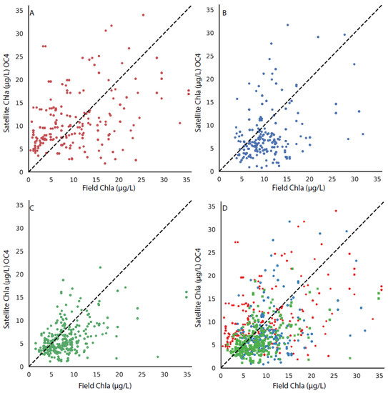
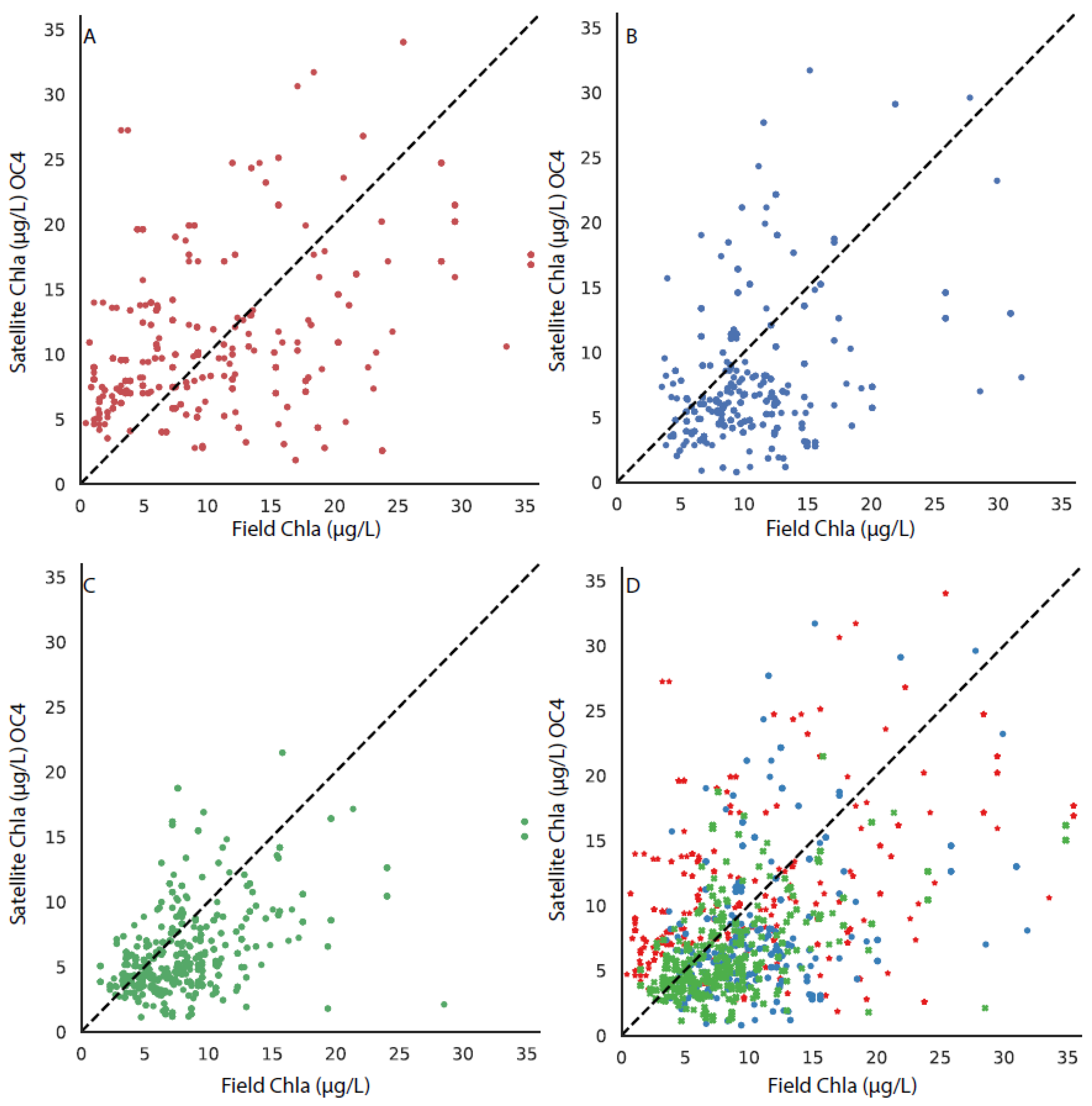
Figure 3.
The matchup between the field chla and the OLCI-OC4 algorithm, with the 1:1 line shown in each subplot for stations in (A) the upper bay, (B) the middle bay, (C) the lower bay, and (D) all stations, with the upper, middle, and lower bays differentiated by symbol color and style.
3.2. Error Metrics between RE10 and OC4
The MAE, MedAE, and their respective biases are described in Section 2.4 and shown in Table 1. Overall, the RE10 bias hovered around 1.04 showing no bias relative to an underestimation of chla when using the OLCI-OC4 algorithm (0.77–0.79). Likewise, the MAE and the MedAE are lower in the RE10 relative to the OLCI-OC4, indicating that there is less error in the RE10 when compared to field estimates of chla. The MedAE indicates an error of approximately 36% when all stations are considered.

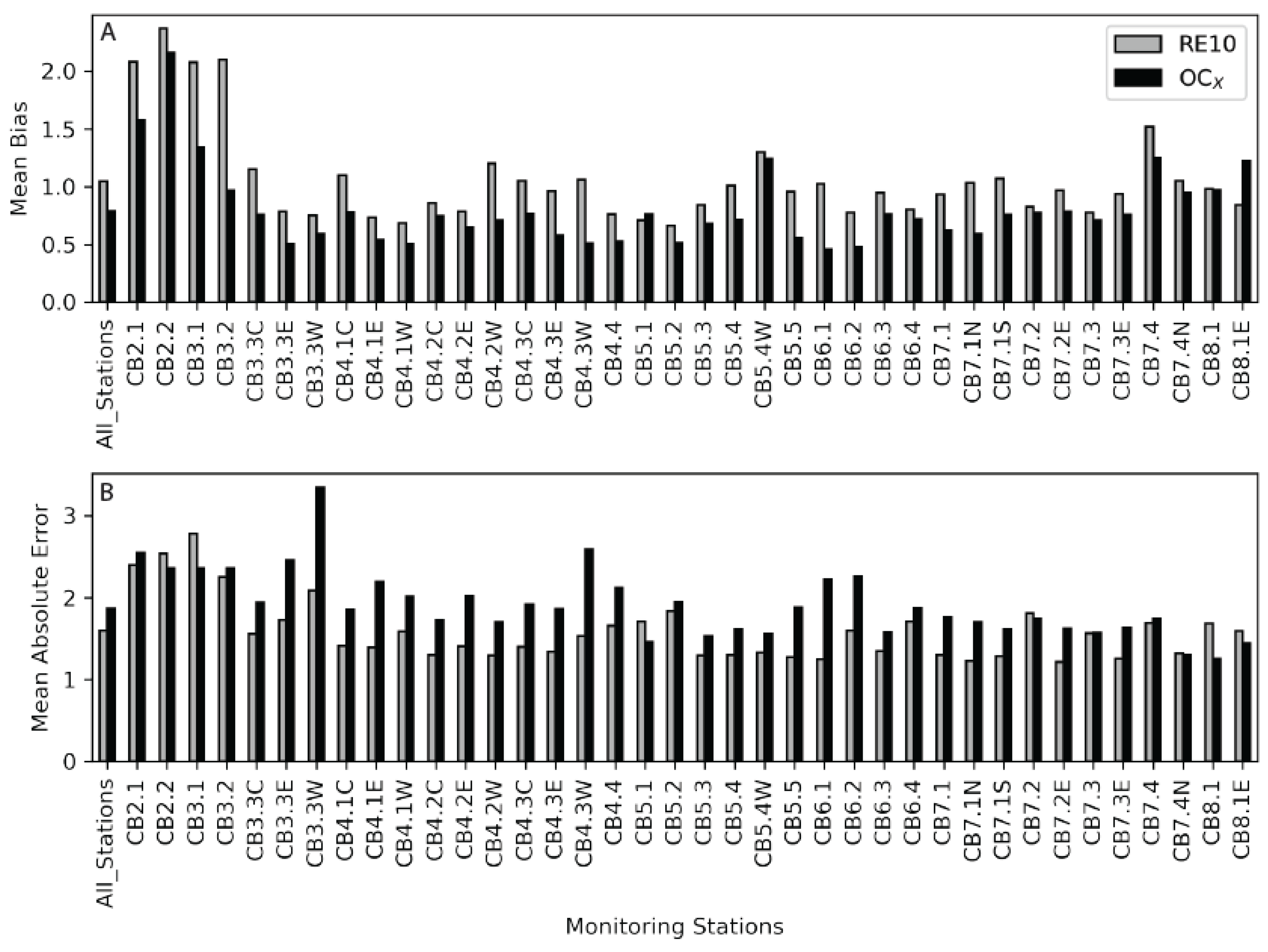
These error estimates vary by station and were plotted to better understand the variability when comparing the upper, middle, and lower regions of the bay (Figure 4 and Figure 5). Stations were plotted from the north (left of the barplot) to south (right of the barplot) and indicated more variability and error in the northern stations. The Median Absolute Error is slightly lower relative to the Mean Absolute Error for both the RE10 and the OLCI-OC4, but both follow similar trends. Differences are related to variability in chla concentration and other factors affecting the water’s optical condition by location. The vast majority of the stations have a lower MAE for the RE10 algorithm relative to the OC4. In 30 stations, the RE10 had a lower MAE error, whereas the OC4 had the lowest MAE in 7 stations, with 1 station (7.3) exhibiting essentially identical error between the two methods. The RE10 algorithm had a lower MAE for 81% of the stations. In 30 stations, the RE10 had a lower MedAE error, whereas the OC4 had the lowest MedAE in 8 stations, indicating that the RE10 algorithm had lower MedAE for 79% of the stations.
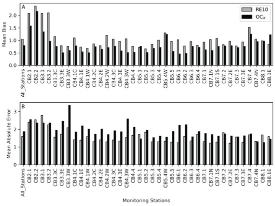
Figure 4.
(A) Mean bias from the field data and the OLCI-RE10 (gray) and the OLCI-OC4 (black) imagery for each station from the Chesapeake Bay Program. The stations run from left to right and represent a transect from the head of the bay to the mouth (Figure 1). Values closer to 1 indicate less bias. (B) The Mean Absolute Error (MAE) is presented in the same fashion as the mean bias.
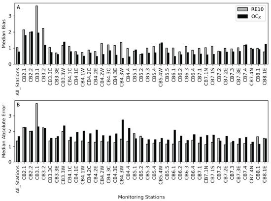
Figure 5.
(A) Median bias from the field data and the OLCI-RE10 (gray) and the OLCI-OC4 (black) imagery for each station from the Chesapeake Bay Program. The stations run from left to right and represent a transect from the head of the bay to the mouth of the bay (Figure 1). Values closer to 1 indicate less bias. (B) The Median Absolute Error (MedAE) is presented in the same fashion as the median bias.
The maximum error for the RE10 algorithm occurs in station 3.1 (Figure 1), which roughly coincides with the location of Chesapeake Bay’s ETM [39]. The ETM is an area of optical complexity and any resultant remotely sensed data should be analyzed with caution in this vicinity. Previous findings by Testa et al. [40] reinforce these results, as they noted a strong influence of CDOM and total suspended sediments (TSS) in low-salinity regions, but a larger role of phytoplankton-associated organic material in meso- and polyhaline regions on water clarity. Station 3.2 is the dividing line where the upper bay transitions to the mid-bay region and is where summer r-values go from ~0.3 to 0.6 between annual and monthly temporal trends. This further illustrates that the optical variability is relatively high north of station 3.2 (Figure 1).
3.3. Matchup in the CoastWatch Suite of OC3 Algorithms
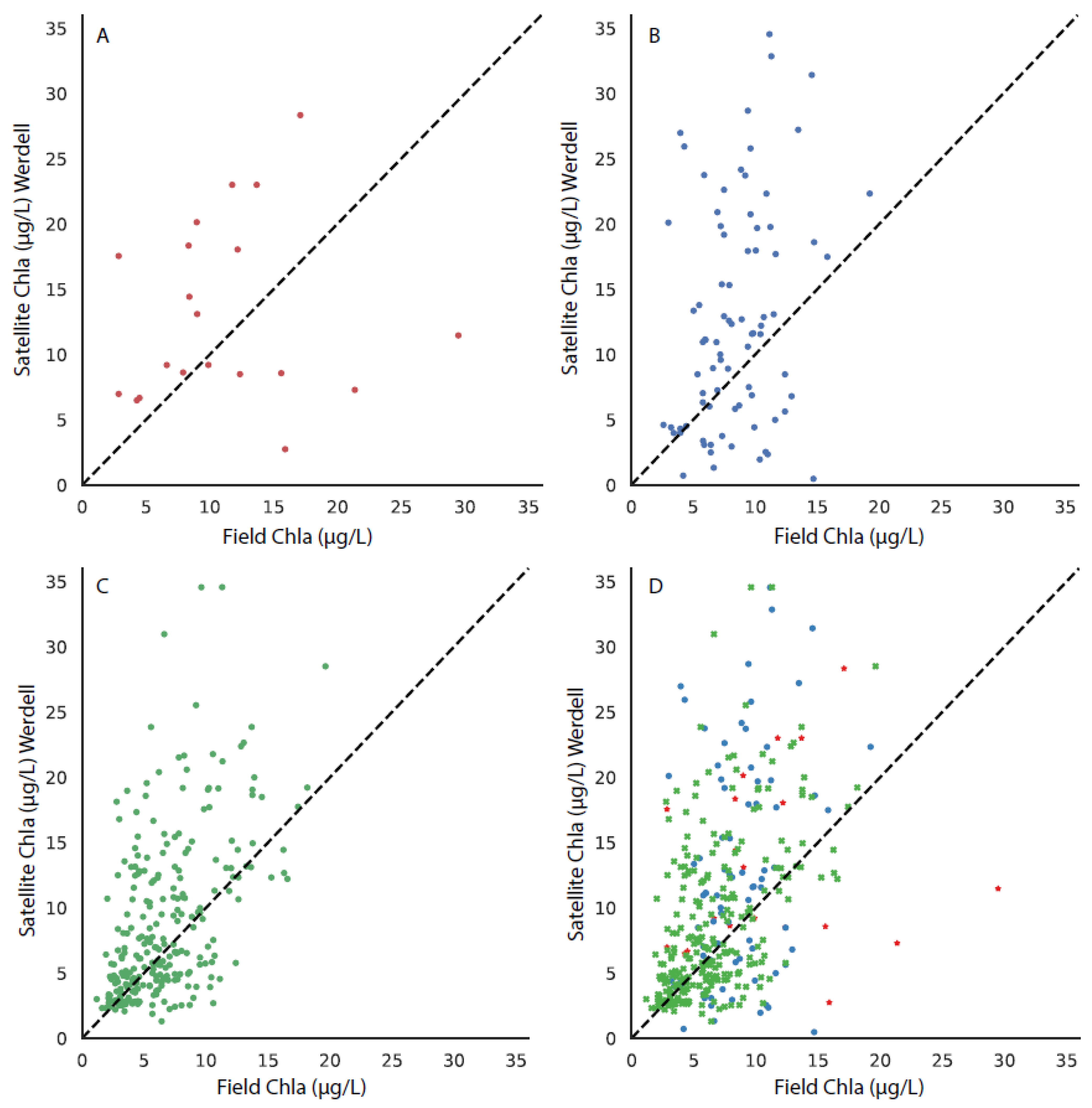
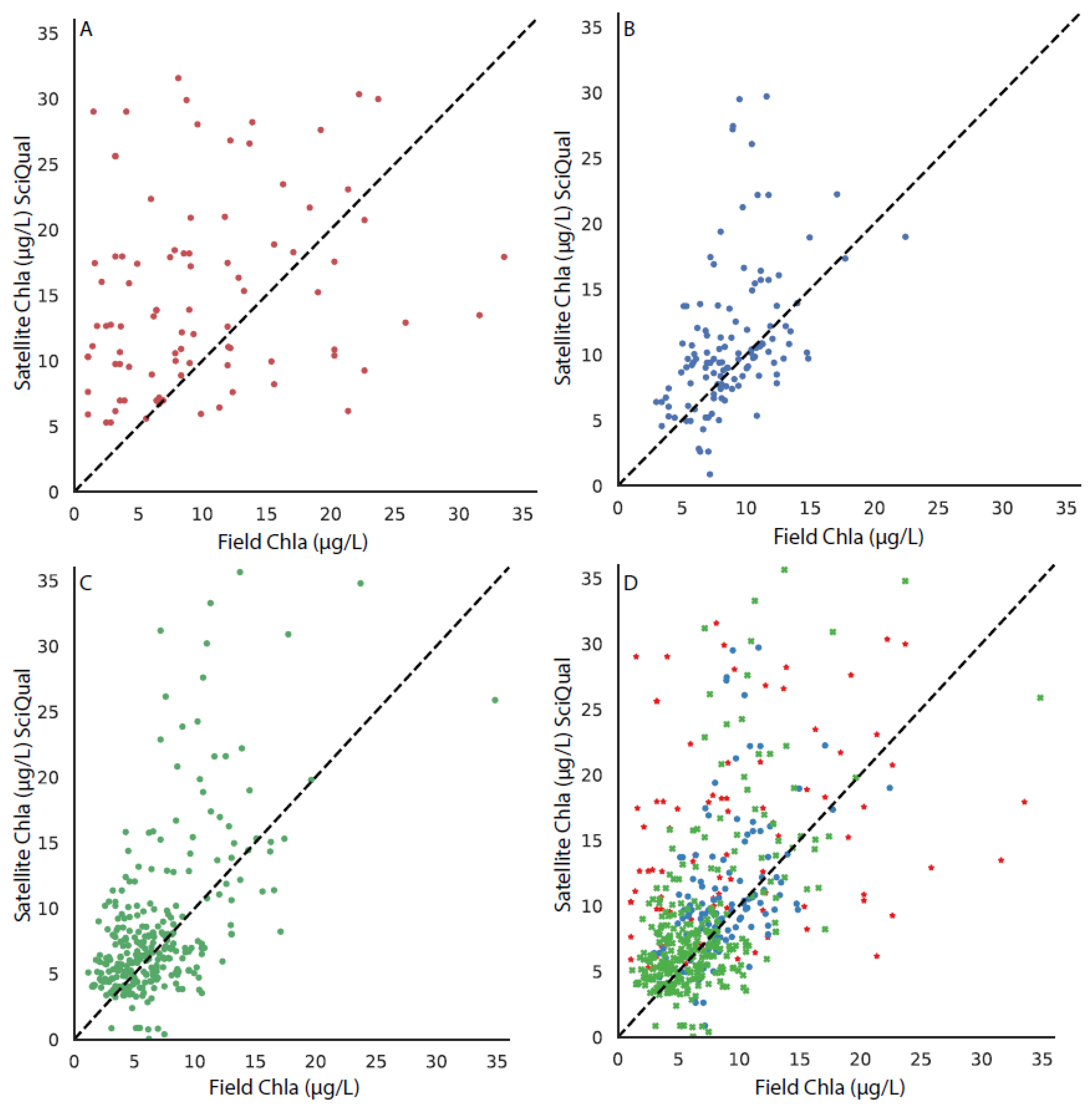
Matchups were performed with the field chla data from the CBP to each of the three CoastWatch suite of OC3 algorithms. The results from the comparison can be seen in Figure 6 (MODIS-Wang), Figure 7 (MODIS-Werdell), and Figure 8 (VIIRS-SciQual). There were fewer coincident field and satellite samples for all three algorithms than the OLCI algorithms (RE10 and OC4). This was partially as a result of the removal of pixels due to a failed atmospheric correction and failures of the OC3 algorithms in areas of high phytoplankton biomass, turbidity, and CDOM. In addition, the influence of clouds and other artifacts has a greater effect in removing pixels for nine 1 km (or 750 m) pixels than for nine 300 m pixels. The results indicate that all three of the CoastWatch algorithms overpredicted the field chla as there were far more points above the one-to-one line in all cases (Figure 6, Figure 7 and Figure 8).
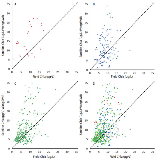
Figure 6.
The matchup between the field chla and the MODIS-Wang algorithm, with the 1:1 line shown in each subplot for stations in (A) the upper bay, (B) the middle bay, (C) the lower bay, and (D) all stations, with the upper, middle, and lower bays differentiated by symbol color and style.
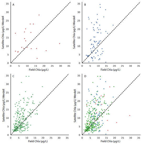
Figure 7.
The matchup between the field chla and the MODIS-Werdell algorithm, with the 1:1 line shown in each subplot for stations in (A) the upper bay, (B) the middle bay, (C) the lower bay, and (D) all stations, with the upper, middle, and lower bays differentiated by symbol color and style.
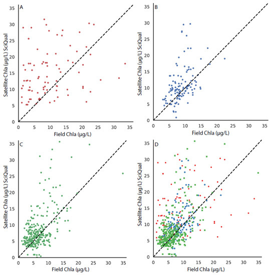
Figure 8.
The matchup between the field chla and the VIIRS-SciQual algorithm, with the 1:1 line shown in each subplot for stations in (A) the upper bay, (B) the middle bay, (C) the lower bay, and (D) all stations, with the upper, middle, and lower bays differentiated by symbol color and style.
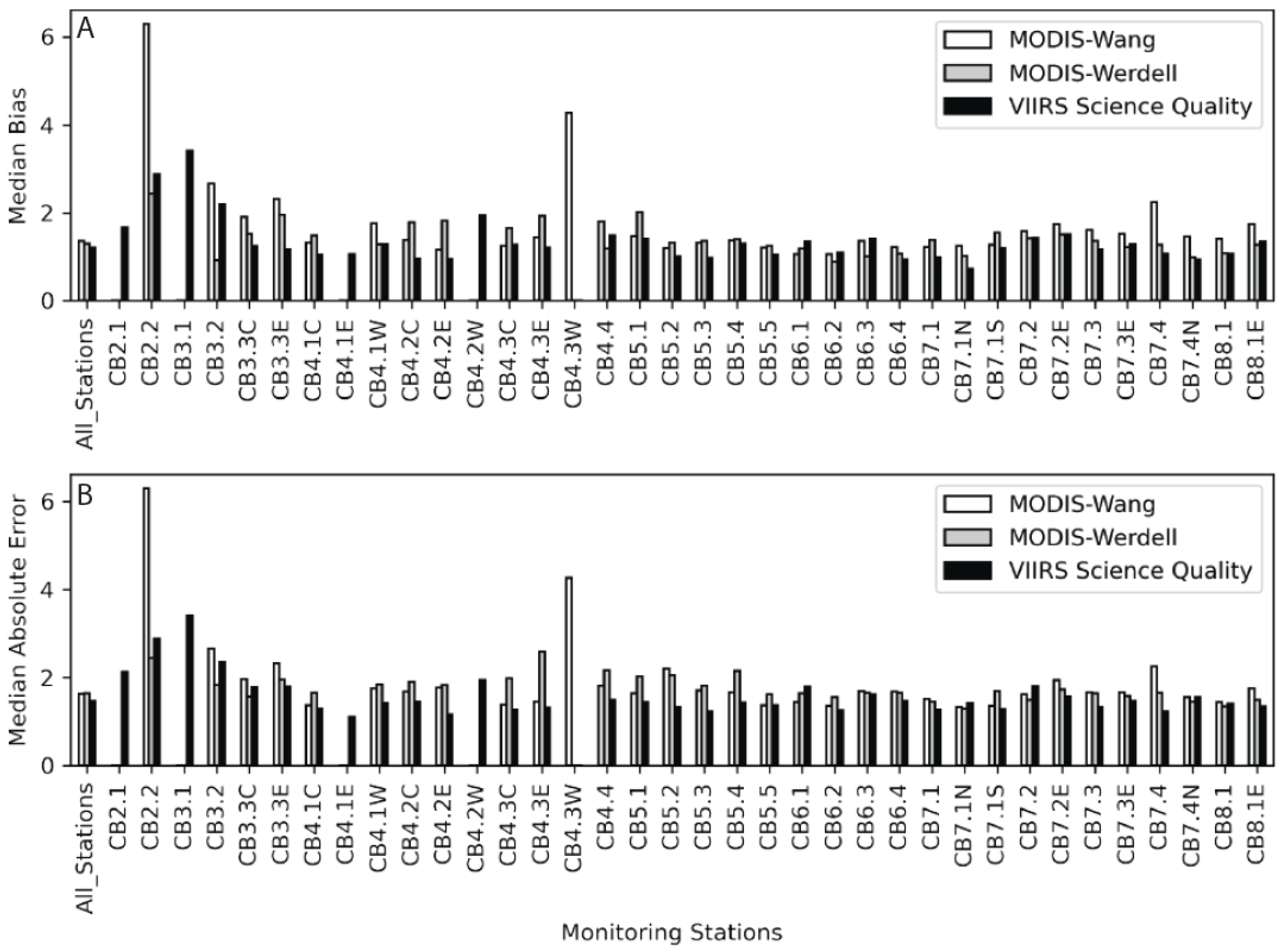
3.4. Error Metrics for the CoastWatch Suite of Algorithms
The mean bias, MAE, median bias, and MedAE were computed for the three algorithms from the CoastWatch suite of data, with the results summarized in Table 2. The VIIRS product outperformed the two MODIS products using all of the metrics described in Section 2.4, as both error terms and both bias terms were closest to one. Both of the MODIS algorithms performed similarly. The OLCI-OC4 algorithm (results shown in Table 1) had results that align with the CoastWatch-provided algorithms in Table 2. The RE10 algorithm outperformed the four different OCx algorithms in all metrics.
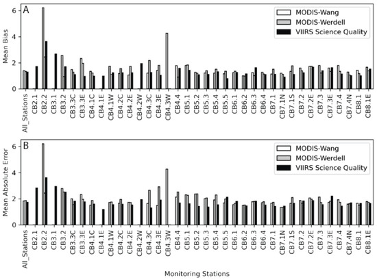
Figure 9.
(A) Mean bias from the field data and the MODIS-Wang (white), MODIS-Werdell (gray), and VIIRS-SciQual (black) imagery for each station from the CBP. The stations run from left to right and represent a transect from the head of the bay to the mouth of the bay (Figure 1). Values closer to 1 indicate less bias. (B) Mean Absolute Error (MAE) is presented in the same fashion as the bias.
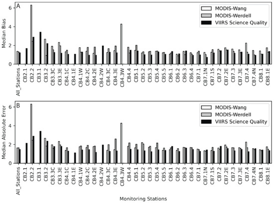
Figure 10.
(A) Median bias from the field data and the MODIS-Wang (white), MODIS-Werdell (gray), and VIIRS-SciQual (black) imagery for each station from the CBP. The stations run from left to right and represent a transect from the head of the bay to the mouth of the bay (Figure 1). Values closer to 1 indicate less bias. (B) Median Absolute Error (MedAE) is presented in the same fashion as the bias.
3.5. Climatological and Time Series Analysis
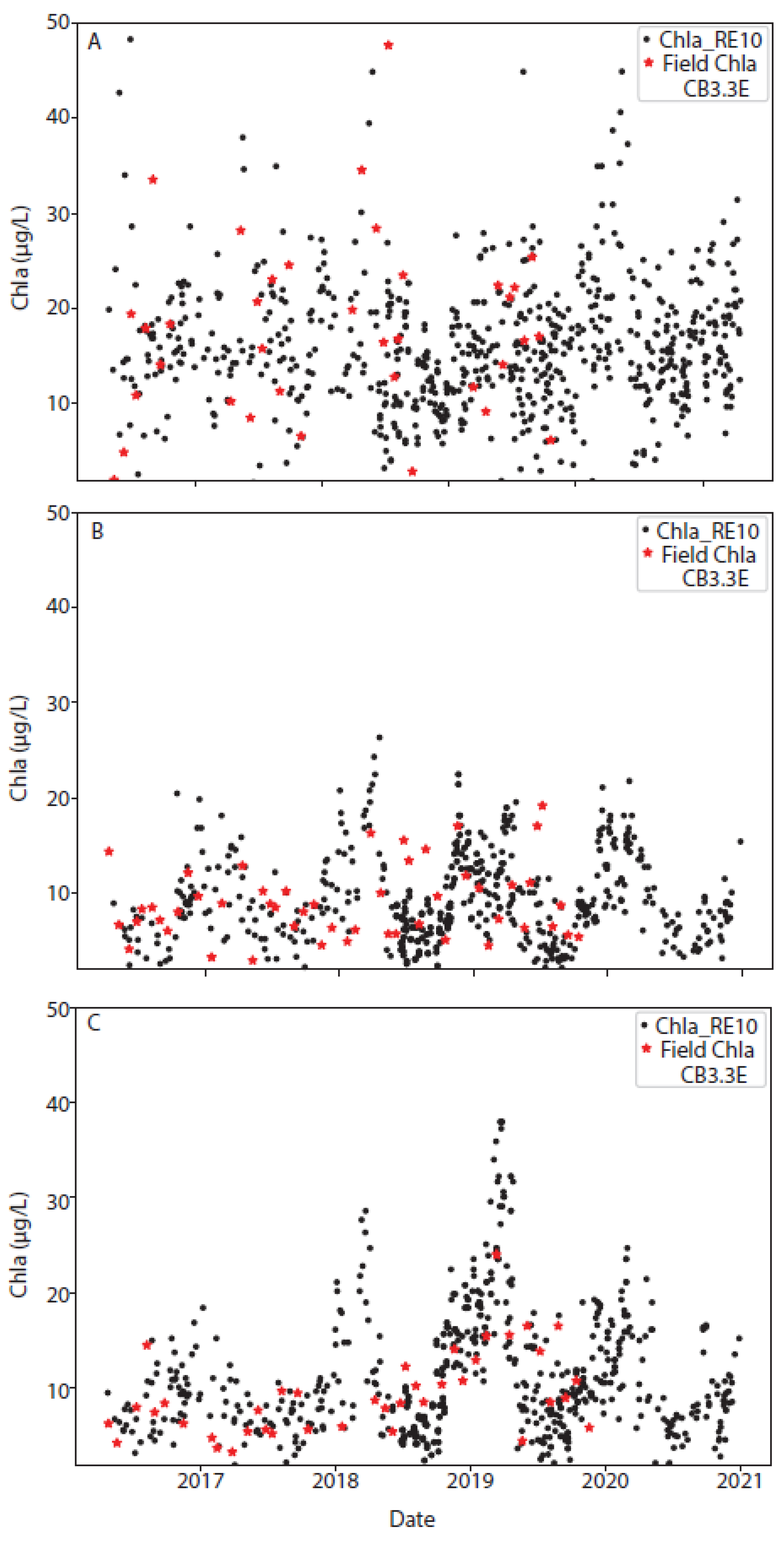
Three representative stations were selected to show the time series of the OLCI-RE10 data along with monthly field chla from the CBP (Figure 11). Overall, these results indicate that the algorithm is stable across years; however, more variability occurs in the northern station 3.3 E (Figure 1), with a larger range in chla concentration. The seasonal cycle in chla is more predominant in the middle and lower bay stations, stations 5.2 and 7.1N, respectively. Due to the influence of the Susquehanna River, variable chla due to increased sediment loading and increased nutrient-induced phytoplankton blooms may be responsible for larger error and bias estimates in the stations surrounding the ETM. For all stations, satellite estimates (black dots) were consistent with field estimates of chla (red stars).
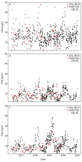
Figure 11.
Time series of the RE10 chla algorithm (black dots) along with any available field data (red stars) for three selected stations: one in the (A) upper bay (station 3.3 E), (B) middle bay (Station 5.2), and (C) lower bay (station 7.1 N). This climatology was calculated using the mean of all data from the start of the Sentinel-3A mission (February 2016) through October 2021. Additional time series graphs for other stations are available in the Supplementary Materials.
4. Discussion
Identifying a robust and reliable chla algorithm for Chesapeake Bay is an important step in the development of many bio-physical algorithms. Submerged aquatic vegetation throughout the bay has been shown to be very sensitive to nitrogen [41], suggesting that seagrass meadows are responsive to inputs of nitrogen. Orth et al. (2010) [41] showed an inverse relationship between point-source nitrogen loads and SAV area. One of the confounding effects of increased nitrogen concentrations is an increase in phytoplankton, leading to a decrease in light availability to the bottom of the water column. Chla can be used as a proxy for phytoplankton concentrations, making it an important model parameter in determining ideal SAV habitat. Another example would be in the calculation of total maximum daily loads (TMDL), which estimate the maximum concentration of a certain pollutant that a water body can receive to meet water quality standards. It can be thought of as the sum of point source pollution and nonpoint source allocations plus a margin of safety. Excess nitrogen (N) and phosphorus (P) can cause eutrophication and therefore can be classified as pollutants. Chla can be used as a proxy for N and P concentrations and can be an input to model various TMDL loading scenarios [4,5]. Excess chla from eutrophication sinks to the benthos, where it is decomposed by bacteria. This decomposition reduces levels of dissolved oxygen in the bottom waters of Chesapeake Bay, causing an area of hypoxia/anoxia which is often referred to as a “dead zone” [40]. Furthermore, reliable chla concentrations can be used for aquaculture site selection [42]. Remotely sensed data have been used for site selection for shellfish [6,43] and finfish [44] abroad as well as in Chesapeake Bay [45]. Furthermore, blooms of potentially toxic harmful algae that can be detrimental to aquaculture can be detected and monitored with remotely sensed data [46].
Harding et al. (2015) showed that in all regions of the bay (upper, middle, and lower), diatoms make up the majority of the floral composition based on pigments in Chesapeake Bay in the spring (~66%) and fall (~49%). The summer floral composition is much more varied with diatoms and dinoflagellates both comprising ~27% of the composition, while cryptophytes account for 18% and cyanobacteria an additional 23%. Harding et al. (2015) [47] also noted that the upper reaches of the bay had a much more diverse phytoplankton community structure. It should be noted that the RE10 algorithm gave predicted results regardless of the floral composition.
One surprising result of this study was that in the very upper reaches of the bay (Stations 2.1, 2.2, and 3.1 in Figure 1), the OLCI-OC4 algorithm outperformed the RE10 algorithm. This region contains the turbidity maximum of the bay, with the highest concentration of sediment. Newell and Fisher (2002) [48] found that in the low salinity reaches of the bay (the head of the bay). the CDOM fluorescence to CDOM absorption ratio was not constant, which suggests the mixing of multiple CDOM sources, which may cause fluctuations in the reflectance spectrum. It has been shown that the chla in the bay is generally inversely correlated with salinity [49], leading to a higher concentration of chla in the upper bay. Higher chla in this region is a result of the Susquehanna River, which delivers half of the freshwater and inorganic nutrients into the bay. The time series analysis shown in Figure 11 indicates that this may be the case as higher chla concentrations were found in the northernmost stations. However, there is a weak correlation between the discharge of the Susquehanna River and the chla concentration [50,51]. Another possible explanation is that RE10 has a strong positive bias for Field chla < 10 µg L−1 (Figure 4), while OC4 has no skill for chla > 10 μg L−1 (Figure 3). If ρs(709) > ρs(665) (which is used to calculate RE10, Equation (1)) for low chla, the apparent discrepancies in the head of the bay values could be explained by atmospheric correction. Alternatively, it is possible that there is so much detrital absorption that it decreases at the water reflectance at 665 nm relative to that at 709 nm.
Using Secchi depth as a proxy for the optical complexity of water, we may be able to infer how remotely sensed chla algorithms respond to the three salinity regimes of Chesapeake Bay (low salinity upper bay, mesohaline middle bay, and polyhaline lower bay). In the upper bay, long-term mean deviations in water clarity most strongly correlated with TSS, in contrast to the middle bay where long-term deviations in water clarity correlated highly with chla [40]. This is indicative of phytoplankton being the primary driver of interannual variability in this area with degraded light conditions. The lower bay stands out because long-term deviations in Secchi depth most strongly corresponded to changes in the ratio of chla:TSS (r = −0.59, p < 0.001), suggesting Secchi depth is lower when phytoplankton-derived material is a larger fractional contributor to TSS. This leads to the assumption that the RE10 algorithm, employed here using Rayleigh-corrected surface reflectance, outperforms OLCI-OC4, regardless of whether a full atmospheric correction (recall that the three CoastWatch-provided algorithms used a full atmospheric correction, while the OLCI-OC4 had a simple correction using the 885 nm band) is present or not when chla is the dominant driver of water turbidity. However, in cases where the water is turbid primarily from TSS, it appears that the OLCI-OC4 algorithm outperforms the RE10 perhaps because of the full atmospheric correction.
It has been shown that primary production in Chesapeake Bay is dependent on the outflow of the Susquehanna River, with wet years being more productive relative to dry years. The Susquehanna provides 80% on N into the bay. In spring, when flow from the Susquehanna is high, P is limiting. In summer, when flow from the Susquehanna is low and there is an increase in the P flux from the sediment, N becomes limiting [47]. To test whether wet or dry years had any role in algorithmic performance, the annual discharge data from 1968–2021 from the Susquehanna River at the head of the bay (USGS station 01578310; Figure 1) at Conowingo was downloaded. Any year in which discharge exceeded the third quartile was considered a wet year, while any year in which discharge was lower than the first quartile was considered a dry year. Years with discharges between the first and third quartiles were considered normal years. Using these definitions, we determined that 2016 was a dry year and 2018 and 2019 were wet years, with the remaining years classified as normal. The RE10 algorithm performed reliably for all years: wet, dry, and normal. This can be seen in Figure 11, with Figure 11B,C showing increased chla in both 2018 and 2019 corresponding to the wet years.
5. Conclusions
In this paper, we have shown that a previously published algorithm [17] provides chla concentrations from OLCI data that are consistent with field spectrometric chla from the Chesapeake Bay Program. The algorithm performs reliably throughout the three regions of the bay: the low salinity upper bay, the mesohaline middle bay, and polyhaline lower bay. The algorithm also performs reliably in wet, dry, and normal years. Furthermore, the increased spatial resolution of the OLCI sensor relative to VIIRS and MODIS would provide invaluable additional data points along the shoreline and cloud edges.
The NOAA CoastWatch program’s mission statement is to provide everyone with easy access to global and regional satellite data products for use in understanding, managing, and protecting ocean and coastal resources, and for assessing impacts of environmental change in ecosystems, weather, and climate. The program routinely produces three chla algorithms for Chesapeake Bay on two sensors. It is recommended that the OLCI-RE10 algorithm be added to their product suite in order to better serve their mission. Due to the improvement both in resolution and accuracy, efforts to provide more accurate chla in Case 2 coastal regions should investigate the application of the RE10 chla product. Future efforts to develop a robust global chla product should investigate providing a switch from RE10 in coastal areas to an OCx algorithm for low chla regions.
Supplementary Materials
The following supporting information can be downloaded at: https://www.mdpi.com/article/10.3390/jmse10081104/s1, Figure S1 shows time series plots of the RE10 chla algorithm (black dots) along with any available field data (red stars) for the remainder of the CBP stations depicted in Figure 1.
Author Contributions
Conceptualization, M.C.T., T.O.B., R.P.S. and T.T.W.; methodology, T.T.W., M.C.T., T.O.B. and R.P.S.; software, A.M., R.L.V. and R.P.S.; validation, S.M., A.M., T.O.B., T.T.W. and M.C.T.; formal analysis, T.T.W., M.C.T., T.O.B. and R.P.S.; investigation, T.T.W., R.P.S., M.C.T., T.O.B., S.M., A.M. and R.L.V.; data curation, A.M. and R.L.V.; writing—original draft preparation, T.T.W., R.P.S., M.C.T., S.M. and R.L.V.; writing—review and editing, T.T.W., M.C.T., R.P.S., S.M. and R.L.V..; visualization, M.C.T., T.O.B., T.T.W. and R.P.S.; supervision, M.C.T.; project administration, M.C.T.; funding acquisition, M.C.T. All authors have read and agreed to the published version of the manuscript.
Funding
Funding provided by the JPSS PGRR Program.
Institutional Review Board Statement
Not applicable.
Informed Consent Statement
Not applicable.
Data Availability Statement
Data is available upon request. The scientific results and conclusions, as well as any views or opinions expressed herein, are those of the authors and do not necessarily reflect official policy or the position of the NOAA or Department of Commerce.
Acknowledgments
The scientific results and conclusions, as well as any views or opinions herein, are those of the authors and do not necessarily reflect the NOAA or Department of Commerce.
Conflicts of Interest
The authors declare no conflict of interest.
References
- Son, S.; Wang, M.; Harding, L.W., Jr. Satellite-measured net primary production in the Chesapeake Bay. Remote Sens. Environ. 2014, 144, 109–119. [Google Scholar] [CrossRef]
- Moore, J.K.; Abbott, M.R. Phytoplankton chlorophyll distributions and primary production in the Southern Ocean. J. Geophys. Res. Ocean. 2000, 105, 28709–28722. [Google Scholar] [CrossRef]
- Hood, R.R.; Shenk, G.W.; Dixon, R.L.; Smith, S.M.; Ball, W.P.; Bash, J.O.; Batiuk, R.; Boomer, K.; Brady, D.C.; Cerco, C. The Chesapeake Bay program modeling system: Overview and recommendations for future development. Ecol. Model. 2021, 456, 109635. [Google Scholar] [CrossRef]
- Tango, P.J.; Batiuk, R.A. Deriving Chesapeake Bay water quality standards. JAWRA J. Am. Water Resour. Assoc. 2013, 49, 1007–1024. [Google Scholar] [CrossRef]
- Liu, Y.; Scavia, D. Analysis of the Chesapeake Bay hypoxia regime shift: Insights from two simple mechanistic models. Estuaries Coasts 2010, 33, 629–639. [Google Scholar] [CrossRef]
- Snyder, J.; Boss, E.; Weatherbee, R.; Thomas, A.C.; Brady, D.; Newell, C. Oyster aquaculture site selection using Landsat 8-Derived Sea surface temperature, turbidity, and Chlorophyll-a. Front. Mar. Sci. 2017, 190. [Google Scholar] [CrossRef]
- USEPA. Ambient Water Quality Criteria for Dissolved Oxygen, Water Clarity and Chlorophyll-a for the Chesapeake Bay and Its Tidal Tributaries: 2007 Addendum, U.S. Environmental Protection Agency Region III Chesapeake Bay Program Office Annapolis. 2009. Available online: https://cdn.ioos.noaa.gov/media/2017/12/ambient_water_quality_criteria.pdf (accessed on 25 June 2022).
- Morel, A.; Prieur, L. Analysis of variations in ocean color 1. Limnol. Oceanogr. 1977, 22, 709–722. [Google Scholar] [CrossRef]
- O’Reilly, J.E.; Maritorena, S.; Mitchell, B.G.; Siegel, D.A.; Carder, K.L.; Garver, S.A.; Kahru, M.; McClain, C. Ocean color chlorophyll algorithms for SeaWiFS. J. Geophys. Res. Ocean. 1998, 103, 24937–24953. [Google Scholar] [CrossRef]
- O’Reilly, J.; Werdell, P. Chlorophyll algorithms for ocean color sensors-OC4, OC5 & OC6. Remote Sens. Environ. 2019, 229, 32–47. [Google Scholar]
- CoastWatch. Available online: https://eastcoast.coastwatch.noaa.gov/region_cd.php#chlor (accessed on 14 April 2022).
- Wang, M.; Shi, W. The NIR-SWIR combined atmospheric correction approach for MODIS ocean color data processing. Opt. Express 2007, 15, 15722–15733. [Google Scholar] [CrossRef]
- Werdell, P.J.; Bailey, S.W.; Franz, B.A.; Harding Jr, L.W.; Feldman, G.C.; McClain, C.R. Regional and seasonal variability of Chlorophyll-a in Chesapeake Bay as observed by SeaWiFS and MODIS-Aqua. Remote Sens. Environ. 2009, 113, 1319–1330. [Google Scholar] [CrossRef]
- Wang, M.; Liu, X.; Jiang, L.; Son, S. The Viirs Ocean Color Product Algorithm Theoretical Basis Document. National Oceanic and Atmospheric Administration, National Environmental Satellite and Data Information Service. 2017. Available online: https://www.nesdis.noaa.gov/ (accessed on 25 June 2022).
- Wright, S.; Jeffrey, S.; Mantoura, R. Phytoplankton Pigments in Oceanography: Guidelines to Modern Methods; Unesco Pub.: Paris, France, 2005. [Google Scholar]
- Pope, R.M.; Fry, E.S. Absorption spectrum (380–700 nm) of pure water. II. Integrating cavity measurements. Appl. Opt. 1997, 36, 8710–8723. [Google Scholar] [CrossRef] [PubMed]
- Gilerson, A.A.; Gitelson, A.A.; Zhou, J.; Gurlin, D.; Moses, W.; Ioannou, I.; Ahmed, S.A. Algorithms for remote estimation of Chlorophyll-a in coastal and inland waters using red and near infrared bands. Opt. Express 2010, 18, 24109–24125. [Google Scholar] [CrossRef] [PubMed]
- CBP. Chesapeake Bay Program: Guide to Using CBP Water Quality Monitoring Data. Available online: https://www.chesapeakebay.net/documents/3676/wq_data_userguide_10feb12_mod.pdf (accessed on 29 October 2021).
- Levinson, A.V.; Li, C.; Royer, T.C.; Atkinson, L.P. Flow patterns at the Chesapeake Bay entrance. Cont. Shelf Res. 1998, 18, 1157–1177. [Google Scholar] [CrossRef]
- Kemp, W.M.; Boynton, W.R.; Adolf, J.E.; Boesch, D.F.; Boicourt, W.C.; Brush, G.; Cornwell, J.C.; Fisher, T.R.; Glibert, P.M.; Hagy, J.D. Eutrophication of Chesapeake Bay: Historical trends and ecological interactions. Mar. Ecol. Prog. Ser. 2005, 303, 1–29. [Google Scholar] [CrossRef]
- Rothschild, B.J.; Ault, J.S.; Goulletquer, P.; Héral, M. Decline of the Chesapeake Bay oyster population: A century of habitat destruction and overfishing. Mar. Ecol. Prog. Ser. 1994, 111, 29–39. [Google Scholar] [CrossRef]
- Wolny, J.L.; Tomlinson, M.C.; Schollaert Uz, S.; Egerton, T.A.; McKay, J.R.; Meredith, A.; Reece, K.S.; Scott, G.P.; Stumpf, R.P. Current and future remote sensing of harmful algal blooms in the Chesapeake Bay to support the shellfish industry. Front. Mar. Sci. 2020, 7, 337. [Google Scholar] [CrossRef]
- Wynne, T.T.; Meredith, A.; Briggs, T.; Litaker, W.; Stumpf, R.P. Harmful Algal Bloom Forecasting Branch Ocean Color Satellite Imagery Processing Guidelines. 2018. Available online: https://www.researchgate.net/publication/331155343_Harmful_Algal_Bloom_Forecasting_Branch_Ocean_Color_Satellite_Imagery_Processing_Guidelines (accessed on 25 June 2022).
- Stumpf, R.P.; Pennock, J.R. Calibration of a general optical equation for remote sensing of suspended sediments in a moderately turbid estuary. J. Geophys. Res. Ocean. 1989, 94, 14363–14371. [Google Scholar] [CrossRef]
- Ioannou, I.; Gilerson, A.; Ondrusek, M.; Foster, R.; El-Habashi, A.; Bastani, K.; Ahmed, S. Algorithms for the remote estimation of Chlorophyll-a in the Chesapeake Bay. In Proceedings of the Ocean Sensing and Monitoring VI; SPIE: Bellingham, WA, USA, 2014; pp. 257–266. [Google Scholar]
- Stumpf, R.P.; Tyler, M.A. Satellite detection of bloom and pigment distributions in estuaries. Remote Sens. Environ. 1988, 24, 385–404. [Google Scholar] [CrossRef]
- Gurlin, D.; Gitelson, A.A.; Moses, W.J. Remote estimation of chl-a concentration in turbid productive waters—Return to a simple two-band NIR-red model? Remote Sens. Environ. 2011, 115, 3479–3490. [Google Scholar] [CrossRef]
- Moses, W.J.; Gitelson, A.A.; Berdnikov, S.; Saprygin, V.; Povazhnyi, V. Operational MERIS-based NIR-red algorithms for estimating Chlorophyll-a concentrations in coastal waters—The Azov Sea case study. Remote Sens. Environ. 2012, 121, 118–124. [Google Scholar] [CrossRef]
- Sentinel. OC4Me Chlorophyll. Available online: https://sentinels.copernicus.eu/web/sentinel/technical-guides/sentinel-3-olci/level-2/oc4me-chlorophyll (accessed on 15 February 2022).
- Siegel, D.A.; Wang, M.; Maritorena, S.; Robinson, W. Atmospheric correction of satellite ocean color imagery: The black pixel assumption. Appl. Opt. 2000, 39, 3582–3591. [Google Scholar] [CrossRef] [PubMed]
- Jiang, L.; Wang, M. Improved near-infrared ocean reflectance correction algorithm for satellite ocean color data processing. Opt. Express 2014, 22, 21657–21678. [Google Scholar] [CrossRef] [PubMed]
- Bailey, S.W.; Franz, B.A.; Werdell, P.J. Estimation of near-infrared water-leaving reflectance for satellite ocean color data processing. Opt. Express 2010, 18, 7521–7527. [Google Scholar] [CrossRef] [PubMed]
- Ruddick, K.G.; Ovidio, F.; Rijkeboer, M. Atmospheric correction of SeaWiFS imagery for turbid coastal and inland waters. Appl. Opt. 2000, 39, 897–912. [Google Scholar] [CrossRef]
- Wang, M.; Shi, W.; Jiang, L. Atmospheric correction using near-infrared bands for satellite ocean color data processing in the turbid western Pacific region. Opt. Express 2012, 20, 741–753. [Google Scholar] [CrossRef]
- Bailey, S.W.; Werdell, P.J. A multi-sensor approach for the on-orbit validation of ocean color satellite data products. Remote Sens. Environ. 2006, 102, 12–23. [Google Scholar] [CrossRef]
- Roman, M.R.; Holliday, D.V.; Sanford, L.P. Temporal and spatial patterns of zooplankton in the Chesapeake Bay turbidity maximum. Mar. Ecol. Prog. Ser. 2001, 213, 215–227. [Google Scholar] [CrossRef]
- Seegers, B.N.; Stumpf, R.P.; Schaeffer, B.A.; Loftin, K.A.; Werdell, P.J. Performance metrics for the assessment of satellite data products: An ocean color case study. Opt. Express 2018, 26, 7404–7422. [Google Scholar] [CrossRef]
- Wynne, T.T.; Mishra, S.; Meredith, A.; Litaker, R.W.; Stumpf, R.P. Intercalibration of MERIS, MODIS, and OLCI Satellite Imagers for Construction of Past, Present, and Future Cyanobacterial Biomass Time Series. Remote Sens. 2021, 13, 2305. [Google Scholar] [CrossRef]
- North, E.; Chao, S.; Sanford, L.; Hood, R. The influence of wind and river pulses on an estuarine turbidity maximum: Numerical studies and field observations in Chesapeake Bay. Estuaries 2004, 27, 132–146. [Google Scholar] [CrossRef]
- Testa, J.M.; Lyubchich, V.; Zhang, Q. Patterns and trends in Secchi disk depth over three decades in the Chesapeake Bay estuarine complex. Estuaries Coasts 2019, 42, 927–943. [Google Scholar] [CrossRef]
- Orth, R.J.; Williams, M.R.; Marion, S.R.; Wilcox, D.J.; Carruthers, T.J.; Moore, K.A.; Kemp, W.M.; Dennison, W.C.; Rybicki, N.; Bergstrom, P. Long-term trends in submersed aquatic vegetation (SAV) in Chesapeake Bay, USA, related to water quality. Estuaries Coasts 2010, 33, 1144–1163. [Google Scholar] [CrossRef]
- Gernez, P.; Palmer, S.C.; Thomas, Y.; Forster, R. remote sensing for aquaculture. Front. Mar. Sci. 2021, 7, 638156. [Google Scholar] [CrossRef]
- Thomas, Y.; Mazurié, J.; Alunno-Bruscia, M.; Bacher, C.; Bouget, J.-F.; Gohin, F.; Pouvreau, S.; Struski, C. Modelling spatio-temporal variability of Mytilus edulis (L.) growth by forcing a dynamic energy budget model with satellite-derived environmental data. J. Sea Res. 2011, 66, 308–317. [Google Scholar] [CrossRef]
- Forget, M.-H.; Stuart, V.; Platt, T. Remote Sensing in Fisheries and Aquaculture; International Ocean Colour Coordinating Group (IOCCG): Dartmouth, NS, Canada, 2009. [Google Scholar]
- Uz, S.S.; Ames, T.J.; Memarsadeghi, N.; McDonnell, S.M.; Blough, N.V.; Mehta, A.V.; McKay, J.R. Supporting aquaculture in the Chesapeake Bay using artificial intelligence to detect poor water quality with remote sensing. In Proceedings of the IGARSS 2020-2020 IEEE International Geoscience and Remote Sensing Symposium, Waikoloa, HI, USA, 17 February 2021; pp. 3629–3632. [Google Scholar]
- Gokul, E.A.; Raitsos, D.E.; Gittings, J.A.; Hoteit, I. Developing an atlas of harmful algal blooms in the red sea: Linkages to local aquaculture. Remote Sens. 2020, 12, 3695. [Google Scholar] [CrossRef]
- Harding Jr, L.; Adolf, J.; Mallonee, M.; Miller, W.; Gallegos, C.L.; Perry, E.; Johnson, J.; Sellner, K.; Paerl, H. Climate effects on phytoplankton floral composition in Chesapeake Bay. Estuar. Coast. Shelf Sci. 2015, 162, 53–68. [Google Scholar] [CrossRef]
- Rochelle-Newall, E.J.; Fisher, T.R. Chromophoric dissolved organic matter and dissolved organic carbon in Chesapeake Bay. Mar. Chem. 2002, 77, 23–41. [Google Scholar] [CrossRef]
- Acker, J.G.; Harding, L.W.; Leptoukh, G.; Zhu, T.; Shen, S. Remotely-sensed chl a at the Chesapeake Bay mouth is correlated with annual freshwater flow to Chesapeake Bay. Geophys. Res. Lett. 2005, 32. [Google Scholar] [CrossRef]
- Le, C.; Hu, C.; Cannizzaro, J.; Duan, H. Long-term distribution patterns of remotely sensed water quality parameters in Chesapeake Bay. Estuar. Coast. Shelf Sci. 2013, 128, 93–103. [Google Scholar] [CrossRef]
- Le, C.; Hu, C.; Cannizzaro, J.; English, D.; Muller-Karger, F.; Lee, Z. Evaluation of Chlorophyll-a remote sensing algorithms for an optically complex estuary. Remote Sens. Environ. 2013, 129, 75–89. [Google Scholar] [CrossRef]


Publisher’s Note: MDPI stays neutral with regard to jurisdictional claims in published maps and institutional affiliations. |
© 2022 by the authors. Licensee MDPI, Basel, Switzerland. This article is an open access article distributed under the terms and conditions of the Creative Commons Attribution (CC BY) license (https://creativecommons.org/licenses/by/4.0/).