Seasonal Evolution of Chlorophyll-a in the North Indian Ocean Associated with the Indian Ocean Dipole and Two Types of El Niño Events

Abstract

To investigate the main modes of interannual variation of chlorophyll-a (Chla) with seasonal evolution and its variation cycle in the North Indian Ocean based on satellite-derived products during 1998–2016, a season-reliant empirical orthogonal function (S-EOF) analysis and power spectrum analysis based on Fourier transform are applied in the study. The first three dominate modes reveal distinct Chla variability, as the S-EOF1 features by one dipole pattern have a negative anomaly in the central western Indian Ocean and a positive anomaly off the Java–Sumatra coasts, which is mainly synchronously associated with the climate indices of the positive Indian Ocean dipole (IOD) and eastern Pacific El Nino (EP-El Niño). The S-EOF2 indicates a tripolar structure with positive anomalies located in the central Indian Ocean surrounded by two negative anomalies, which is one year behind a positive IOD and EP-El Niño event. The S-EOF3 exhibits a different dipole distribution, with a positive anomaly in the central west and a negative anomaly in the southeast, synchronized or lagging behind the central Pacific El Nino (CP-El Niño). Moreover, regarding the correlation between the main modes of interannual variation and the IOD and El Nino events, the dynamic parameters (such as SST, SLA, rain, and wind) of the tropical Indo-Pacific Ocean are discussed using time-delay correlation and linear regression analysis to explain the key factors and possible influencing mechanism of the joint seasonal and interannual variations of Chla in the northern Indian Ocean.

1. Introduction

The Northern Indian Ocean is significantly influenced by monsoons and monsoonal circulations and has one of the highest primary productivities in the world. In recent years, domestic and foreign scholars have carried out many studies on the spatio-temporal variation characteristics of the concentration of chlorophyll-a (Chla) in the Northern Indian Ocean [1,2,3,4,5,6]. Wiggert et al. [2] found that an increase in Chla in the 5° S–12° S latitude sea area in the boreal summer was caused by the combined action of local Ekman pumping and Rossby waves. Wiggert et al. [6] compared the variation characteristics of Chla in the tropical Indian Ocean during two positive IOD events and found that the positive anomaly of Chla occurred in the southern part of the Bay of Bengal, while the negative anomaly occurred in most of the Arabian Sea. Barimalala et al. [3] analyzed SeaWiFS water color data and found that during El Nino events, Chla in the Arabian Sea decreased by 24% in winter, and positive IOD events reduced Chla by 20% in autumn. Liao [5] analyzed the phytoplankton blooms in summer and winter in the tropical Western Indian Ocean and their influencing mechanisms. However, previous studies have focused on the seasonal or interannual variations of Chla in the Indian Ocean, while there have been few studies on the seasonal evolution characteristics of Chla in the northern Indian Ocean.

The Indian Ocean dipole (IOD) is an east–west oscillation mode of SST anomalies in the equatorial Indian Ocean. It generally occurs in the northern hemisphere summer, matures in autumn, dies out in winter, and affects the variation characteristics of the ocean biomass in the Indian Ocean on a seasonal–interannual scale. ENSO can have a profound impact on the northern Indian Ocean through atmospheric and oceanic bridges [7,8]. According to reports, El Nino events can be divided into two types, namely, the eastern Pacific type and the central Pacific type. Different from the traditional eastern El Nino phenomenon, the central El Nino is characterized by the abnormal warming of the SST in the central equatorial Pacific. However, there have been few studies on the influence of different types of El Nino events on the upper ocean environment of the tropical Indian Ocean [9,10,11,12].

Therefore, the aim of this paper was to identify the dominant seasonal evolutions of interannual Chla variation in the North Indian Ocean during 1998–2016 and to investigate their responses to the climate variability of IOD and two types of El Niño, as well as the ocean dynamic anomalies of the SST, sea surface height anomaly (SLA), sea surface rainfall (Rain), and wind field (Wind).

2. Materials and Methods

2.1. Materials

Various remote sensing products were used to measure the variables, which included Chla, SST, SLA, Rain, and Wind, whose sources, timespans, and resolutions are summarized in

Table 1. Sources, timespans, and resolutions of remote sensing datasets.

Variable	Data Source	Timespan	Resolution
Chla	OC-CCI V3.1 [13]	September 1997–present	4 km, monthly
SST	OI SST V2.0 [14]	December 1981–present	0.25°, daily
SLA	AVISO	December 1992–present	0.25°, monthly
Rain	GPCP V2.3 [15]	January 1979–present	2.5°, monthly
Wind	CCMP V2.0 [16]	January 1987–present	0.25°, monthly

.

In addition, the Indian Ocean Dipole Index (DMI), which represents IOD events and is calculated from the difference in the mean SST across the equatorial Indian Ocean in the western (50°–70° E, 10° S–10° N) and eastern (90°–110° E, 10° S–0) regions, was also used. NinoCE indices for the Central Pacific and Eastern Pacific types of ENSO were used to directly distinguish the two ENSO events, namely NinoCE = (NinoEP, NinoCP). Among them, the calculation methods for NinoEP (eastern index, representing cold-tongue ENSO) and NinoCP (middle index, representing warm-pool ENSO) are equivalent to the cold-tongue index (CTI) and warm-pool index (WPI), respectively, defined by [12]. The data were obtained from the National Climate Center, China Meteorological Administration (https://cmdp.ncc-cma.net/pred/cn_enso.php?product=cn_enso_nino_indices accessed on 22 May 2022). When the DMI and NinoCE were positive, El Nino/positive IOD (PIOD) events occured, while negative values indicate that La Nina/negative IOD (NIOD) events occurred. The interannual curves of the DMI and NinoCE indices are shown in Figure 1.

2.2. Methods

The Chla maps were firstly resampled to 0.25° for computational efficiency and log10 transformed due to their lognormal distribution [17]. Then, season-reliant empirical orthogonal function (S-EOF) analysis, explained in detail by B. Wang and An [18], was applied to the Chla anomalies. Season-reliant empirical orthogonal function (S-EOF) analysis involves arranging the distance square matrix of the Chla according to the following form: X(x, t) = [x^JJA(t), x^SON(t), x^DJF(t), x^MAM(t)], where the t stands for the year, JJA stands for boreal summer (June, July, August), SON stands for boreal autumn (September, October, November), DJF stands for boreal winter (December, January, February), MAM stands for boreal spring (March, April, May). JJA(0), SON(0), D(0)JF(1), and MAM(1) are defined as the consecutive boreal summer, autumn, winter, and spring of year (0) of the current year, where 0 denotes the year before year 1. Then X(x, t) was decomposed by the conventional EOF, and each eigenvector obtained contained the evolution features of four seasons: summer, autumn, winter, and spring. Each eigenvector was divided into four consecutive vectors to obtain the modes of the seasonal evolution of Chla. The continuous modes of these four seasons correspond to the same principal component.

Power spectrum analysis based on Fourier transform was also used to identify the oscillation period of the dominant seasonal evolution modes. In addition, we employed the lead–lag correlation and linear regression methods to investigate the Chla variability associated with climate indices and ocean dynamic variables.

3. Results

3.1. Dominant Seasonal Evolution Patterns of Chla in the North Indian Ocean

The seasonal climate distribution of Chla in the northern Indian Ocean during the years 1998–2016 is shown in Figure 2. It can be seen that the high-value Chla area is mainly concentrated in the western and northern Indian Ocean, and there is a significant seasonal shift in the high-value area, while the central and southern equatorial regions are always low.

The S-EOF analysis was performed on the seasonal anomaly sequence of Chla from 1998 to 2016, and the first three modes with physical significance were obtained. The variance contribution rates were 18.28%, 14.54%, and 7.68%, respectively, and the total variance contribution rate was 40.5%. Fourier transform-based power spectrum analysis was performed on the corresponding time series of principal components (PCs). The spatial mode (S-EOF), PC, and power spectrum analysis results are shown in Figure 3, Figure 4 and Figure 5. The first three modes reflect the main characteristics of the interannual variation of Chla in the northern Indian Ocean, along with the seasonal evolution.

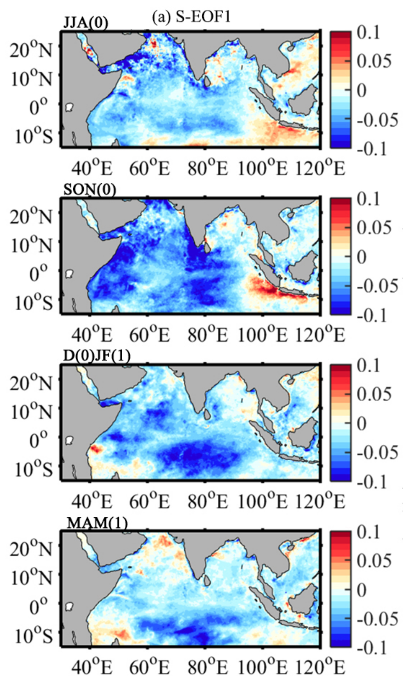
The spatial pattern of S-EOF1 (Figure 3a) shows that Chla in the northern Indian Ocean was dominated by negative anomalies on the whole, and significant positive anomalies were detected along the Java–Sumatra coasts, and both positive and negative Chla anomaly centers and intensity varied greatly with seasons. It is very different from the seasonal climate distribution of Chla (high values are concentrated in the western and northern Indian Ocean in Figure 1), indicating the significant interannual variation characteristics of this mode. In the boreal summer (Figure 3a, JJA(0)), positive and negative Chla anomalies began to appear in the Java–Sumatra and central western Indian Ocean waters, respectively. In the boreal autumn (Figure 3a, SON(0)), the Chla variation increased, and the intensity and range of the negative anomaly reached the maximum. In the boreal winter and spring (Figure 3a, D(0)JF(1), MAM(1)), the Chla intensity of the negative anomaly weakened and the positive range increased.

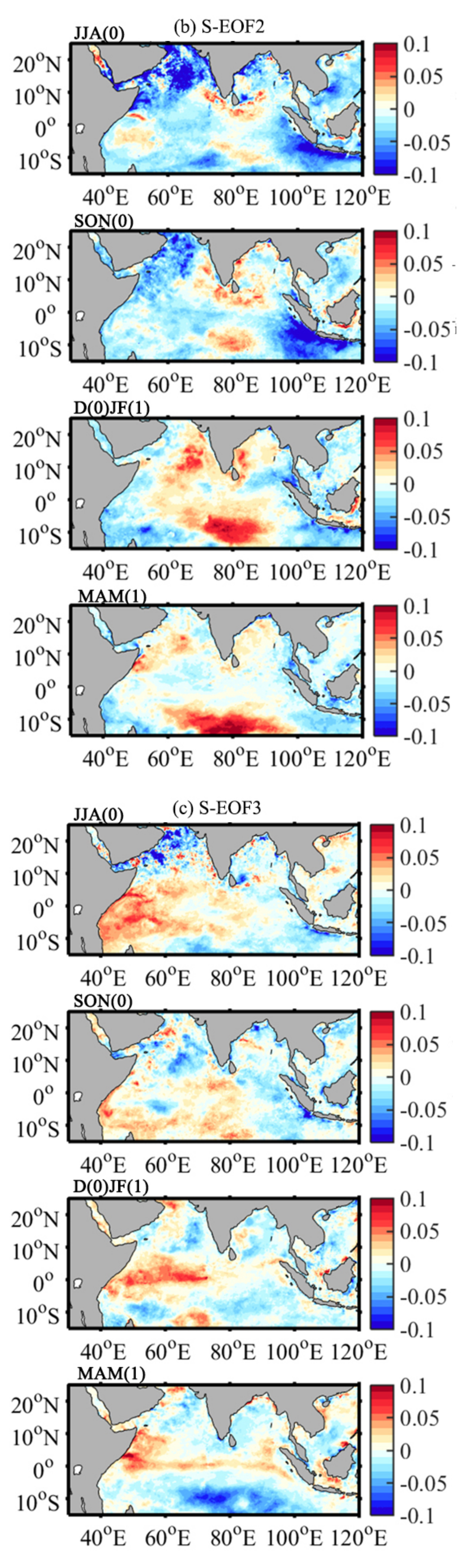
Figure 3b shows the spatial pattern of S-EOF2 with significant positive seasonal Chla variation in the central Indian Ocean, and the negative anomaly centers mainly appear in the western Arabian Sea and the Java–Sumatra coasts. During the boreal summer (Figure 3b, JJA(0)), the positive Chla anomaly began to appear in the western equatorial Indian Ocean, the southern Indian Peninsula, the waters near Sri Lanka, and the central Indian Ocean at the latitude of 10° S. The significant negative anomaly centers were distributed in the central Arabian Sea and the Java–Sumatra coastal waters. During the boreal autumn (Figure 3b, SON(0)), the positive Chla anomaly increased significantly, while the negative anomaly intensity and range reached the maximum along the Java–Sumatra coasts. During the boreal winter (Figure 3b, D(0)JF(1)), the Chla continued to rise, maximizing the range and intensity of the positive anomalies.

Meanwhile, the spatial pattern of S-EOF3 (Figure 3c) features a dipole distribution, with a positive anomaly in the western Indian Ocean, a negative anomaly along the coast of the Java–Sumatra island in the 10° S latitude zone, and the intensity of the positive anomaly was significantly higher than that of the negative anomaly. The seasonal variation of Chla is relatively complicated. In the boreal summer (Figure 3c, JJA(0)), the significant positive anomaly of Chla occurred in the western equatorial Indian Ocean, and the significant negative anomaly occurred in the northwestern Arabian Sea. In the boreal autumn (Figure 3c, SON(0)), the negative anomaly intensity of Chla decreased, and its center moved southward in the Arabian Sea, while the negative anomaly in the Java–Sumatra coast moved northward, and the positive anomaly intensity decreased in the western equatorial Indian Ocean and moved eastwards to the central equatorial Indian Ocean.

To summarize, the S-EOF1 pattern shows that Chla, on the whole, features mostly negative anomalies and varies greatly with seasons, with obvious positive anomalies detected off the Java–Sumatra coasts. The negative and positive anomalies appeared separately in the central western Indian Ocean and the Java–Sumatra coasts during the boreal summer, with the maximum variability observed in the boreal autumn. A tripolar structure, with positive anomalies located in the central Indian Ocean and surrounded by two negative anomalies in the northwest and southeast, is recorded in the S-EOF2 pattern. Both positive and negative anomalies developed remarkably with the seasons and peaked in the boreal winter and autumn, respectively. The S-EOF3 pattern features a dipole distribution with a positive anomaly in the central west and a negative anomaly in the southeast, on the whole, accompanied by a relatively complex variability transition from an east–west to a north–south anomaly with seasons.

Figure 4 shows a time series of the principal components, and the magnitude of the absolute value reflects the strength of the variation. The greater the absolute value is, the stronger the variation is at that moment and the more typical the spatial distribution pattern is. In addition, if the time coefficient is negative, it means that the spatial distribution pattern of the moment is opposite to that shown in the figure. As shown in Figure 4a, the time coefficients of PC1 are all negative from 1998 to 2005, except in 1999 and 2000, and positive from 2006 to 2015, except in 2007 and 2010. Among them, the negative values in 2005 and 2010 and the positive values in 2012 and 2015 are the most prominent. The results show that the Chla in the northern Indian Ocean had strong variation during these four years. 2015 was a year of strong El Nino and positive IOD events. Together with Figure 3a (SON(0)), it can be seen that the Chla in the northern Indian Ocean presents a typical dipole variation structure with negative anomalies in the central west and positive anomalies in the east, indicating that the simultaneous occurrence of El Nino and positive IOD events strengthened the inter-annual variation of the Chla in the northern Indian Ocean. However, the time coefficient of 2012 is smaller than that of 2015, indicating that the dipole variation structure was weaker than that of 2015, mainly because 2012 was a year of strong positive IOD events and weak La Nina events, and La Nina events may have weakened the Chla variation intensity in the northern Indian Ocean. Similarly, the time coefficient in 2005 was significantly negative, indicating that the Chla in the northern Indian Ocean experienced a variation structure opposite to that in Figure 3a (SON(0)), that is, the Chla in the central and western Indian Ocean was positively abnormal, and the Chla in the Java–Sumatra coast was negatively abnormal, which positively corresponds to the negative IOD events in 2005. The absolute value of the time coefficient in 2010 is smaller than that in 2005, and the interannual variation at this time was also smaller than that in 2005, while 2010 was a year of negative IOD and strong La Nina events, which also indicates that the occurrence of La Nina events weakened the varying intensity of the Chla in the northern Indian Ocean. In conclusion, the first main mode of the Chla change in the northern Indian Ocean is the one closely associated with the IOD and ENSO events.

PC2 shows negative anomalies from 2002 to 2011 (except 2010), positive anomalies from 1998 to 2001 and from 2012 to 2015 (Figure 4b). Among them, the most prominent time coefficients are positive anomalies from 1998 and 2010 and negative anomalies from 2006. In 1998, the time coefficient reached the maximum, and the spatial distribution generally shows a positive anomaly of Chla in the central Indian Ocean and a negative anomaly in the western Arabian Sea and the Java–Sumatra coast (Figure 3b), while 1998 had a negative IOD and La Nina event year. The results show that the simultaneous occurrence of the negative IOD and La Nina events led to a significant increase in the Chla in the central Indian Ocean and a significant decrease in the western Arabian Sea and the Java–Sumatra coast. The year 2010 also had negative IOD and La Nina events, and the above abnormal Chla also occurred, but the intensity was weaker than that of 1998. Similarly, the 2006 negative anomaly shows a decrease in Chla in the central Indian Ocean and an increase along the Java–Sumatra coast. It is shown that the second main mode is also the interannual variation mode associated with the IOD and ENSO events.

The variation characteristics of negative anomalies from 1998 to 2000, positive anomalies from 2001 to 2005, negative anomalies from 2006 to 2012 (except 2009), and positive anomalies from 2013 to 2015 are presented in Figure 4c. The time coefficient values are most significant in 1999, 2011 (negative anomaly), and 2014 (positive anomaly). The year 2014 had positive IOD and El Nino events. In the boreal autumn, the Chla increased (positive anomaly) in the central equatorial Indian Ocean, and in the boreal winter, the Chla significantly increased in the equatorial belt of the western Indian Ocean. In 2011 (positive IOD and La Nina event years), the time coefficient is significantly negative, and the spatial structure of abnormal Chla in the northern Indian Ocean is opposite to that shown in Figure 3c, that is, in the boreal winter, the Chla in the equatorial belt of the western Indian Ocean mainly decreased significantly (negative anomaly). Contrary to the spatial structure of 2014 (positive IOD and El Nino event year), this indicates that ENSO events had a greater influence on the mode, and the third main mode can be considered as the mode associated with ENSO events.

The power spectrum analysis of the time coefficient PC1 shows that the first mode mainly had intra-seasonal oscillation for a period of 6 months and interannual oscillation for a period of 2–2.5 years (Figure 5a), while the oscillation at other time scales was not significant, further indicating the significant interannual variation of Chla in the first mode. The second mode was similar to the first main mode and mainly had seasonal oscillation for a period of 6 months and annual oscillation for a period of 2 years (Figure 5b). However, the power spectrum analysis of the time coefficient PC3 indicates that the third mode only fluctuated significantly in the 6-month and 12-month periods, which is mainly intra-seasonal and annual scale oscillation (Figure 5c), and no inter-annual or longer scale oscillations were detected, which may have been caused by the short Chla dataset (only 19 years).

3.2. Lead–Lag Correlations between Dominant S-EOF Modes and Climate Indices

The first three main modes of Chla in the northern Indian Ocean have been proven to be associated with IOD events in the Indian Ocean and ENSO events in the Pacific Ocean, but the relationship between them and the two types of El Nino events (eastern and central type) could not be determined. Therefore, the lead–lag correlations calculated for further determining relationships between the dominant S-EOF modes and climate indices of DMI, NinoEP, and NinoCP are shown in Figure 6, where Y(−1), Y(1), and Y(0) represent PC of Chla lags, leads one year and synchronizes to the climate index, respectively.

It can be seen from the diagram of the lead–lag correlation coefficients between the first three main mode time series and the DMI (Figure 6a) that the correlation coefficient between PC1 and DMI (red broken line) passed the 95% confidence test in the same year during JJA(0)–SON(0) (boreal summer–autumn), with a significant positive correlation, and the maximum correlation coefficient is 0.67, which appears in the boreal autumn. The correlation coefficient between PC2 and DMI (green broken line) passed the significance test of SON(-1)–DJF(-1) in the previous year, and the maximum correlation coefficient is 0.4. According to the seasonal phase-locking characteristics of IOD events, that is, the development in the boreal spring and summer, the peak in the boreal autumn, and the decline in the boreal winter, the first and second main modes of Chla in the northern Indian Ocean were associated with the development process of IOD events, indicating that the S-EOF1 synchronously correlated with the IOD, while the S-EOF2 mainly lagged by one year.

Figure 6b shows the time-delay correlation coefficient with NinoEP. It can be seen that the correlation coefficient between PC1 and NinoEP (red broken line) passed the significance test in JJA(0)–SON(0)–DJF(0) of the same year, indicating that the first main mode was contemporaneous with the eastern El Nino event. The correlation coefficient between PC2 and NinoEP (green broken line) passed the significance test of JJA(−1)–SON(−1)–DJF(−1) in the previous year, and reached the maximum value in the boreal winter with a correlation coefficient of 0.70. Considering the seasonal phase-locking of ENSO events (development in the boreal spring and summer, maturity in the boreal autumn and winter), The second main mode is correlated with the lag of eastern El Nino events, that is, the interannual variation of the second main mode lags behind the occurrence of eastern El Nino events by one year. In addition, the correlation coefficient between PC3 and NinoEP (blue broken line) passed the significance test of SON(1)–DJF(1) a year later, indicating that the third main mode is correlated with the eastern El Nino event one year before.

The time-delay correlation coefficient with NinoCP is shown in Figure 6c. It can be seen that the correlation coefficient (blue broken line) between PC3 and NinoCP passed the significance test in the boreal summer, autumn, winter, and spring of the previous year and in the same year, and reached the maximum value at DJF(0), the correlation coefficient is 0.83. The results indicate that the third main mode is correlated with the central El Nino events lagging one year behind or in the same period, which means that the central El Nino events have a significant influence on the interannual variation of the third main mode of Chla in the northern Indian Ocean.

On the whole, the IOD and ENSO events have a close connection with the interannual variation of Chla in the northern Indian Ocean. The S-EOF1 synchronously correlated with the IOD, while the S-EOF2 mainly lagged by one year. Similarly, S-EOF1 and S-EOF2 were also found to co-occur with and lag behind EP-El Niño events, respectively, whereas S-EOF3 was primarily synchronized with or lagged behind CP-El Niño events.

3.3. Seasonal Evolution Patterns of Dynamic Anomalies Associated with Dominant S-EOF Modes

According to Section 3.2, the first main mode of the interannual variation of Chla in the northern Indian Ocean was synchronously correlated with the DMI and NinoEP index, while the second main mode lagged behind the DMI and NinoEP index by one year, and the third main mode was found to co-occur with and lagged behind the NinoCP index. In order to explore the key factors and possible influencing mechanisms of the main modes of the interannual variation of Chla in the Indian Ocean under climate change, linear regression analysis was adopted. The linear regression between the main modes of interannual variation of Chla and the dynamic parameters of the tropical Indo-Pacific ocean, including the SST, SLA, Rain, and Wind, was studied. The results of the regression coefficients are shown in Figure 7, Figure 8 and Figure 9.

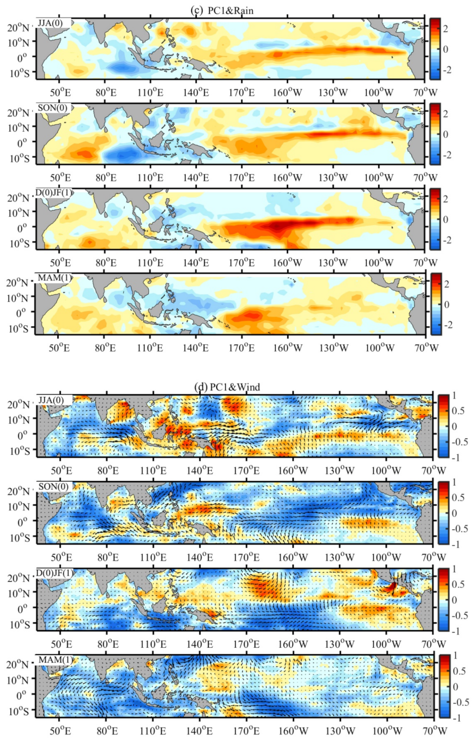
The simultaneous regression coefficients of the first main mode time series (PC1) of Chla in the northern Indian Ocean and the dynamic parameters in the tropical Indo-Pacific ocean are shown in Figure 7. The seasonal evolution of each parameter reflects the development process of typical positive IOD events in the Indian Ocean and El Nino events in the eastern Pacific Ocean. In the Pacific Ocean region, from the boreal summer to winter, the SST and SLA in the middle eastern equatorial Pacific continued to rise, reached the peak at the mature stage of El Nino in the boreal winter, and returned to normal in the boreal spring. Meanwhile, the SST and SLA in the waters near the Indonesian islands significantly decreased (Figure 7a,b). Figure 7c reveals the seasonal evolution of negative precipitation anomalies and positive precipitation anomalies in the South Pacific Convergence Zone (SPCZ), extending northeast from New Guinea to the central Tropical Pacific [19,20]. The surface wind field was mainly manifested by a strong westerly anomaly over the western equatorial Pacific and an easterly anomaly over the eastern Pacific.

In the Indian Ocean area, in the boreal summer and fall, the western equatorial Indian Ocean heating appears to be consistent with that of the eastern equatorial Pacific. The southeastern Indian Ocean sea surface temperature negative anomaly, for the typical Indian Ocean IOD mode, is a response to ENSO events in the Indian Ocean, and its mechanism is the impact of the middle eastern tropical Pacific on the Indian Ocean sea surface heat flux through the “bridge” atmosphere [21]. The sea surface height is also shown as abnormal increases in the western and eastern Indian Oceans and an abnormal decrease in the southeastern Indian Ocean. Meanwhile, the rainfall on the sea surface formed a dipole structure with positive anomalies in the west and negative anomalies in the east. The easterly anomalies in the tropical Indian Ocean produced a westward ocean current, which led to strong upwelling along the coast of Java–Sumatra Island. East wind anomalies exacerbate the abnormal cooling of SST in the southeastern Indian Ocean [22]. All these environmental factors are conducive to the growth of phytoplankton off the coast of the Java–Sumatra Island, resulting in an abnormal increase in the Chla in the sea area. The study shows that during the eastern El Nino, the abnormal increase in the SST in the equatorial eastern Pacific affected the atmospheric circulation system, resulting in the formation of the Walker circulation ascending branch in the central Pacific and the Walker circulation descending branch in the western Pacific to the eastern Indian Ocean, which then affected the local climate system in the tropical Indian Ocean. Easterly anomalies prevail in the whole Indian Ocean. The eastern El Nino weakens the Walker circulation and generates abnormal easterly winds along the Java–Sumatra coast, which is conducive to the development of positive IOD events [23,24].

The parameter regression coefficient of the PC2 that lags behind the tropical Indo-Pacific ocean dynamic is shown in Figure 8. It can be seen that the seasonal evolution is similar to that shown in Figure 7, and it shows that the second main mode is associated with positive IOD events and east Pacific El Niño events. However, the anomalous distribution and intensity of each parameter are quite different, and the anomalous intensity of the second main mode is relatively weak, which is consistent with the correlation research results of the main mode and climate factors discussed in Section 3.2.

In the boreal autumn and winter, the positive SST and SLA anomalies in the equatorial Pacific decreased east of 175° W, and the negative SST and SLA anomalies in the eastern Indian Ocean and western Pacific increased. The variation of the ocean environment in the upper Indian Ocean is obviously different from the first main mode, which was mainly manifested as an abnormal increase in the SST and SLA in the western Indian Ocean, a significant decrease in the SST and SLA in the central Indian Ocean, an abnormal decrease in precipitation in the central and eastern Indian Ocean, and a strong southeastern wind anomaly in the central Indian Ocean. The increase in cold water in the central Indian Ocean, the increase in nutrients in the upper water, and the abnormal increase in phytoplankton biomass are favorable, but phytoplankton growth was inhibited and the Chla decreased significantly along the Java–Sumatra coast.

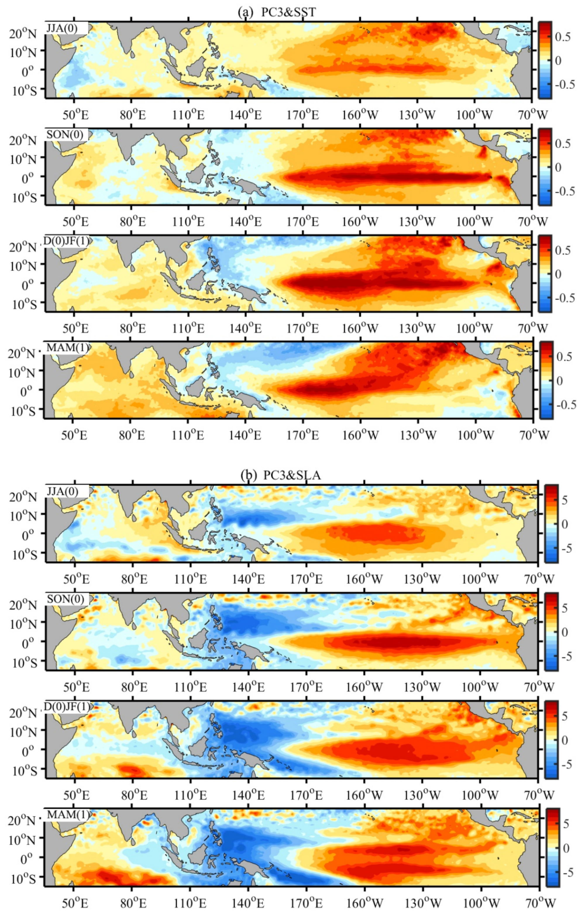
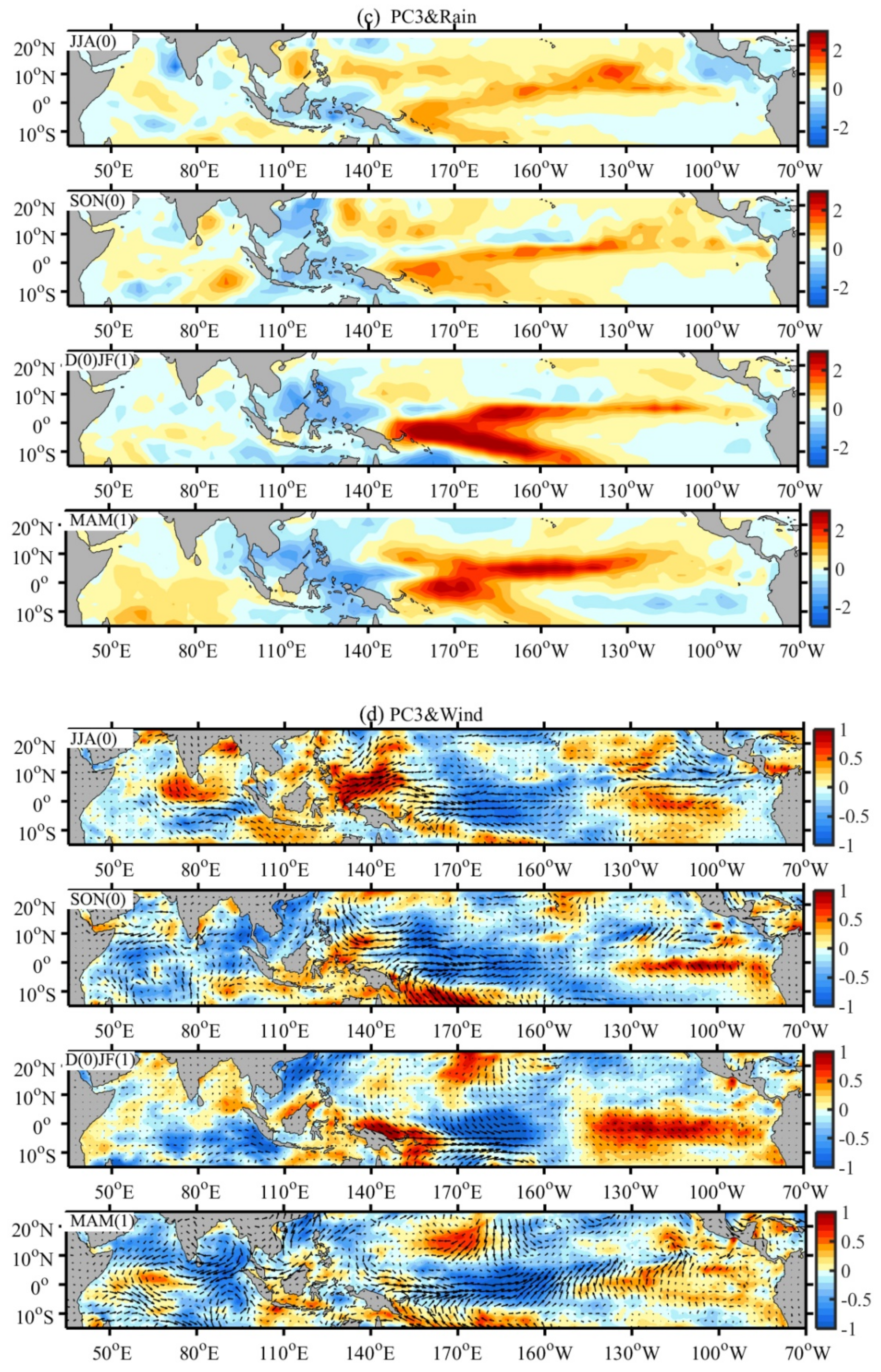
The synchronous regression coefficients of the third main mode of the Indian Ocean Chla (PC3) with the tropical Indo–Pacific Ocean parameters are shown in Figure 9. It can be seen that this mode is different from the first and second modes and only reflects the typical central Pacific Nino events. The incident intensity is bigger and longer, and it can last from the boreal summer of the previous year to the boreal spring of the current year, which is consistent with the correlation results shown in Section 3.2.

Regarding the Pacific Ocean region, Figure 9a shows the seasonal evolution characteristics of the central El Nino in the northern hemisphere starting in the summer, developing in the autumn, maturing in the winter, and fading in the spring. Specifically, the strong abnormal warming begins in the central tropical Pacific and the west coast of the United States in the boreal summer [9]. The positive SST anomaly expands eastward along the equator in the boreal autumn, and the negative SST anomaly extends to the Kuroshio Extension area and the coast of the Indonesian archipelago and reaches the maximum in the boreal winter. The sea surface height shows an abnormal decrease in the tropical western Pacific and an abnormal increase in the tropical central eastern Pacific [25,26]. The Pacific Intertropical Convergence Zone (ITCZ) and the South Pacific Convergence Zone (SPCZ) are positive precipitation anomalies, and negative precipitation anomalies are found in the vicinity of the Indonesian islands. The range of negative precipitation anomalies continues to expand in the boreal autumn, and both positive and negative precipitation anomalies reach the maximum in the boreal winter (Figure 9c). Figure 9d reveals the tropical Walker circulation and the change in the wind field in the mid-latitude Pacific Ocean. In the boreal summer, the strengthening of anomalous westerly winds in the equatorial western Pacific and anomalous easterly winds in the eastern Pacific are conducive to the continuous rise of the SST in the central eastern Pacific, and the weakening of the trade winds in the central tropical Pacific is also conducive to an increase in precipitation [27,28].

In the Indian Ocean, the SST and SLA centers are mainly located in the south central Indian Ocean, while the SST, SLA, and Rain are negative in the western Indian Ocean, and the SLA is negative in the equatorial belt. At the same time, the Indian Ocean is mainly controlled by the abnormal west risk, which can cause a southeast current, so the concentration of Chla in the western Indian Ocean is abnormally expanding to the east. This is not conducive to the development of upwelling along the Sumatra coast, so the phytoplankton biomass along the Sumatra coast is greatly reduced. Studies have shown that a central El Nino can enhance the Walker circulation, resulting in westerly anomalies along the coast of the Java–Sumatra Island. The negative anomaly of the wind speed increases SST, which is not conducive to IOD events [10].

4. Discussion

In this study, we investigated the seasonal evolution characteristics and change cycles of the main modes of interannual variation of Chla in the northern Indian Ocean during 1998–2016 using S-EOF and power spectrum analysis based on Fourier transform. The correlation between the main modes of interannual variation and the IOD, El Nino events, and the dynamic parameters (such as the SST, SLA, Rain, and Wind) of the tropical Indo-Pacific ocean were also discussed using time-delay correlations and linear regression analysis to explain the key factors and possible influencing mechanism of the spatio-temporal variations of Chla in the northern Indian Ocean.

There exist three distinct seasonal evolving modes of the interannual Chla variation in the northern Indian Ocean. In the first mode, the dipole structure of Chla was a negative anomaly in the center and a positive anomaly in the east, and the maximum variation occurred in the boreal autumn, which is associated with the seasonal evolution of positive IOD events (synchronous) and eastern El Nino events (synchronous). The simultaneous regression coefficients reflect the development process of typical positive IOD events in the Indian Ocean and El Nino events in the eastern Pacific Ocean. In the boreal summer and fall, the equatorial western Indian Ocean heating appears to have been consistent with that of the eastern equatorial Pacific, and the southeastern Indian Ocean SST negative anomaly is the typical Indian Ocean IOD mode, which is a response to ENSO events in the Indian Ocean. The mechanism is the impact of the middle eastern tropical Pacific on the Indian Ocean sea surface heat flux through the “bridge” atmosphere [21]. The SLA also shows an abnormal increase in the western and eastern Indian Oceans and an abnormal decrease in the southeastern Indian Ocean. Meanwhile, the rainfall on the sea surface formed a dipole structure with positive anomalies in the west and negative anomalies in the east. The easterly anomalies in the tropical Indian Ocean produced a westward ocean current, which led to strong upwelling along the coast of the Java–Sumatra Island. East wind anomalies exacerbate the abnormal cooling of the SST in the southeastern Indian Ocean [22]. All these environmental factors are conducive to the growth of phytoplankton off the coast of the Java–Sumatra Island, resulting in an abnormal increase in Chla in the sea area. During an eastern El Nino, the abnormal increase in the SST in the equatorial eastern Pacific affected the atmospheric circulation system, resulting in the formation of a Walker circulation ascending branch in the central Pacific and a Walker circulation descending branch in the western Pacific to the eastern Indian Ocean, which then affected the local climate system in the tropical Indian Ocean. Easterly anomalies prevailed across the entire Indian Ocean. An eastern El Nino weakened the Walker circulation and generated abnormal easterly winds along the Java–Sumatra coast, which is conducive to the development of positive IOD events [23,24].

The second main mode shows significant positive seasonal variation of Chla in the central Indian Ocean, while negative anomaly centers mainly appeared in the western Arabian Sea and the Java–Sumatra coast, which also corresponds to the development process of positive IOD events (lagging) and eastern El Nino events (lagging). However, the variation of the ocean environment in the upper Indian Ocean is obviously different from the first main mode, which was mainly manifested as an abnormal increase in the SST and SLA in the western Indian Ocean, a significant decrease in the SST and SLA in the central Indian Ocean, an abnormal decrease in precipitation in the middle and eastern Indian Ocean, and a strong southeast wind anomaly in the central Indian Ocean. The increase in cold water in the central Indian Ocean, the increase in nutrients in the upper water, and the abnormal increase in phytoplankton biomass were favorable, but phytoplankton growth was inhibited and the Chla decreased significantly along the Java–Sumatra coast.

The third main mode is a response to the seasonal evolution of the central El Nino event (synchronous or lagged). The regression coefficients show that the Indian Ocean is mainly controlled by the abnormal west risk, which can cause a southeast current, so the Chla in the western Indian Ocean is abnormally expanding to the east. This is not conducive to the development of upwelling along the Sumatra coast, so the phytoplankton biomass along the Sumatra coast has been greatly reduced. Studies have shown that the central El Nino can enhance the Walker circulation, resulting in westerly anomalies along the coast of the Java–Sumatra Island. The negative anomaly of the wind speed increased the SST, which is not conducive to IOD events [10].

To summarize, IOD and ENSO events have been proven to be closely connected to the interannual variation of Chla in the northern Indian Ocean. The regression coefficients of the main modes of the interannual variation of Chla in the northern Indian Ocean and the dynamic parameters in the tropical Indo-Pacific ocean show that different types of El Nino events have different effects on the upper ocean environment in the Indian Ocean. However, the current research was focused on the discovery of the spatio-temporal variation of Chla in the northern Indian Ocean and the spatio-temporal correlation of eco-dynamic parameters in the tropical Indo-Pacific ocean, but there are still many limitations to explaining the physical mechanism behind these seasonal and interannual variations and correlations. In addition, the ocean dynamic environment in the northern Indian Ocean is very complex and is affected not only by large-scale wind fields but also by short-scale events such as mesoscale eddies. Therefore, the interaction mechanisms among the chlorophyll A concentration, dynamic parameters, and climate factors need to be further studied in the future.

5. Conclusions

Using S-EOF, lead–lag correlation, and power spectrum analyses, we investigated the dominant seasonal evolutions of interannual Chla variations in the northern Indian Ocean during 1998–2016 and their relationships with the IOD and two types of El Niño, providing a new perspective to the understanding of phytoplankton responses to climate change and important guidance for rational fishery exploitation.

We found three distinct evolving seasonal modes, including a dipole pattern with a negative anomaly in the central western Indian Ocean and a positive anomaly off the Java–Sumatra coasts (S-EOF1), a tripolar structure with positive anomalies located in the central Indian Ocean and surrounded by two negative anomalies (S-EOF2), and another dipole distribution with a positive anomaly in the central western and a negative anomaly in the southeastern Indian Ocean (S-EOF3). The S-EOF1 and S-EOF2 modes show significant variation periods of 2–2.5 years, which is similar to those of IOD and ENSO events, whereas the S-EOF3 has 6-month and 12-month variation periods, without inter-annual oscillation detected. The results suggest that the IOD and two types of El Niño are the primary factors for the interannual Chla variations, and different types of El Nino events have different impacts on the upper ocean environment of the Indian Ocean. An eastern El Nino weakens the Walker circulation and produces abnormal easterly winds along the Java–Sumatra coast, which is conducive to the development of positive IOD events and leads to positive abnormal Chla in the central eastern Indian Ocean. A central El Nino can enhance the Walker circulation, resulting in a westerly wind anomaly along the Java–Sumatra coast, which is not conducive to IOD events, and a positive anomaly of Chla in the western Indian Ocean. Regressed anomalies of the dynamic variables (SST, SLA, Rain, and Wind) with the dominant modes can explain the major processes involved in the Chla variability under climate change, though the detailed underlying mechanisms still need to be investigated and clarified in future work.

References

1. Dwi Susanto, R.; Marra, J. Effect of the 1997/98 El Niño on Chlorophyll a Variability along the Southern Coasts of Java and Sumatra. Oceanography 2005, 18, 124–127. [Google Scholar] [CrossRef]
2. Wiggert, J.D.; Murtugudde, R.G.; Christian, J.R. Annual Ecosystem Variability in the Tropical Indian Ocean: Results of a Coupled Bio-Physical Ocean General Circulation Model. Deep Sea Res. Part II Top. Stud. Oceanogr. 2006, 53, 644–676. [Google Scholar] [CrossRef]
3. Barimalala, R.; Bracco, A.; Kucharski, F.; McCreary, J.P.; Crise, A. Arabian Sea Ecosystem Responses to the South Tropical Atlantic Teleconnection. J. Mar. Syst. 2013, 117–118, 14–30. [Google Scholar] [CrossRef] [Green Version]
4. Currie, J.C.; Lengaigne, M.; Vialard, J.; Kaplan, D.M.; Aumont, O.; Naqvi, S.W.A.; Maury, O. Indian Ocean Dipole and El Niño/Southern Oscillation Impacts on Regional Chlorophyll Anomalies in the Indian Ocean. Biogeosciences 2013, 10, 6677–6698. [Google Scholar] [CrossRef] [Green Version]
5. Liao, X.; Ma, J.; Zhan, H. Effect of Different Types of El Niño on Primary Productivity in the South China Sea. Aquat. Ecosyst. Health Manag. 2012, 15, 135–143. [Google Scholar] [CrossRef]
6. Wiggert, J.D.; Vialard, J.; Behrenfeld, M.J. Basin-Wide Modification of Dynamical and Biogeochemical Processes by the Positive Phase of the Indian Ocean Dipole during the SeaWiFS Era. Geophys. Monogr. Ser. 2009, 185, 385–407. [Google Scholar] [CrossRef]
7. Klein, S.A.; Soden, B.J.; Lau, N.-C. Remote Sea Surface Temperature Variations during ENSO: Evidence for a Tropical Atmospheric Bridge. J. Clim. 1999, 12, 917–932. [Google Scholar] [CrossRef] [Green Version]
8. Alexander, M.A.; Bladé, I.; Newman, M.; Lanzante, J.R.; Lau, N.C.; Scott, J.D. The Atmospheric Bridge: The Influence of ENSO Teleconnections on Air-Sea Interaction over the Global Oceans. J. Clim. 2002, 15, 2205–2231. [Google Scholar] [CrossRef]
9. Ashok, K.; Behera, S.K.; Rao, S.A.; Weng, H.; Yamagata, T. El Niño Modoki and Its Possible Teleconnection. J. Geophys. Res. Ocean. 2007, 112, 1–27. [Google Scholar] [CrossRef]
10. Wu, Y.; Liu, L.; Zhang, X.; Duan, Y.; Yang, G.; Yang, Y.; Zahid; Oloo, P.; Sagero, P. Different Impacts from Various El Niño Events on Wyrtki Jets in Boreal Autumn Season. Pure Appl. Geophys. 2018, 175, 4567–4577. [Google Scholar] [CrossRef]
11. Wiedermann, M.; Radebach, A.; Donges, J.F.; Kurths, J.; Donner, R.V. A Climate Network-Based Index to Discriminate Different Types of El Niño and La Niña. Geophys. Res. Lett. 2016, 43, 7176–7185. [Google Scholar] [CrossRef] [Green Version]
12. Ren, H.L.; Jin, F.F. Niño Indices for Two Types of ENSO. Geophys. Res. Lett. 2011, 38, 2–6. [Google Scholar] [CrossRef]
13. Lou, J.F.; Chen, M.; Li, Y.; Peng, T.; Xu, H. Influence of the Two Types of ENSO Events on Seasonal Precipitation over Mid-Dle and Lower Reaches of the Yangtze River. South-to-North Water Transf. Water Sci. Technol. 2018, 4, 82–89. [Google Scholar]
14. Sathyendranath, S.; Brewin, R.J.W.; Brockmann, C.; Brotas, V.; Calton, B.; Chuprin, A.; Cipollini, P.; Couto, A.B.; Dingle, J.; Doerffer, R.; et al. An Ocean-Colour Time Series for Use in Climate Studies: The Experience of the Ocean-Colour Climate Change Initiative (OC-CCI). Sensors 2019, 19, 4285. [Google Scholar] [CrossRef] [Green Version]
15. Reynolds, R.W.; Smith, T.M.; Liu, C.; Chelton, D.B.; Casey, K.S.; Schlax, M.G. Daily High-Resolution-Blended Analyses for Sea Surface Temperature. J. Clim. 2007, 20, 5473–5496. [Google Scholar] [CrossRef]
16. Adler, R.F.; Sapiano, M.R.P.; Huffman, G.J.; Wang, J.J.; Gu, G.; Bolvin, D.; Chiu, L.; Schneider, U.; Becker, A.; Nelkin, E.; et al. The Global Precipitation Climatology Project (GPCP) Monthly Analysis (New Version 2.3) and a Review of 2017 Global Precipitation. Atmosphere 2018, 9, 138. [Google Scholar] [CrossRef] [Green Version]
17. Mears, C.A.; Scott, J.; Wentz, F.J.; Ricciardulli, L.; Leidner, S.M.; Hoffman, R.; Atlas, R. A Near-Real-Time Version of the Cross-Calibrated Multiplatform (CCMP) Ocean Surface Wind Velocity Data Set. J. Geophys. Res. Oceans 2019, 124, 6997–7010. [Google Scholar] [CrossRef]
18. Wang, B.; An, S.-I. A Method for Detecting Season-Dependent Modes of Climate Variability: S-EOF Analysis. Geophys. Res. Lett. 2005, 32, 1–4. [Google Scholar] [CrossRef] [Green Version]
19. Curtis, S. The El Niño-Southern Oscillation and Global Precipitation. Geogr. Compass 2008, 2, 600–619. [Google Scholar] [CrossRef]
20. Liu, C.; Allan, R.P. Multisatellite Observed Responses of Precipitation and Its Extremes to Interannual Climate Variability. J. Geophys. Res. Atmos. 2012, 117, 1–16. [Google Scholar] [CrossRef] [Green Version]
21. He, K.; Liu, G.; Wu, R.; Nan, S.; Wang, S.; Zhou, C.; Qi, D.; Mao, X.; Wang, H.; Wei, X. Oceanic and Land Relay Effects Linking Spring Tropical Indian Ocean Sea Surface Temperature and Summer Tibetan Plateau Precipitation. Atmos. Res. 2022, 266, 105953. [Google Scholar] [CrossRef]
22. Bin, W.; Renguang, W.; Xiuhua, F. Pacific–East Asian Teleconnection: How Does ENSO Affect East Asian Climate? J. Clim. 2000, 13, 1517–1536. [Google Scholar]
23. Wang, X.; Wang, C. Different Impacts of Various El Niño Events on the Indian Ocean Dipole. Clim. Dyn. 2014, 42, 991–1005. [Google Scholar] [CrossRef]
24. Wang, C.; Wang, X. Classifying El Niño Modoki I and II by Different Impacts on Rainfall in Southern China and Typhoon Tracks. J. Clim. 2013, 26, 1322–1338. [Google Scholar] [CrossRef]
25. Delcroix, T. Observed Surface Oceanic and Atmospheric Variability in the Tropical Pacific at Seasonal and ENSO Timescales: A Tentative Overview. J. Geophys. Res. Oceans 1998, 103, 18611–18633. [Google Scholar] [CrossRef]
26. Chang, Y.T.; Du, L.; Zhang, S.W.; Huang, P.F. Sea Level Variations in the Tropical Pacific Ocean during Two Types of Recent El Niño Events. Glob. Planet. Chang. 2013, 108, 119–127. [Google Scholar] [CrossRef]
27. Hou, X.; Dong, Q.; Xue, C.; Wu, S. Seasonal and Interannual Variability of Chlorophyll-α and Associated Physical Synchronous Variability in the Western Tropical Pacific. J. Mar. Syst. 2016, 158, 59–71. [Google Scholar] [CrossRef]
28. Pan, J.; Yan, X.H.; Zheng, Q.; Liu, W.T. Vector Empirical Orthogonal Function Modes of the Ocean Surface Wind Variability Derived from Satellite Scatterometer Data. Geophys. Res. Lett. 2001, 28, 3951–3954. [Google Scholar] [CrossRef]
Figure 1. The interannual curves of DMI and NinoCE indexes, which were all treated with a moving average for 13 months.
Jmse 10 00997 g001
Figure 2. Seasonal average distribution of Chla in the Northern Indian Ocean during January 1998–December 2016 (unit: Log10, mg/m3). (a) Summer (JJA); (b) autumn (SON); (c) winter (DJF); (d) spring (MAM).
Jmse 10 00997 g002
Figure 3. Seasonally evolving spatial patterns of the first three S-EOF modes of Chla from JJA(0) to MAM(1).
Jmse 10 00997 g003aJmse 10 00997 g003b
Figure 4. The normalized principal component (PC) of the first three S-EOF modes with interpolated time series (black curve).
Jmse 10 00997 g004
Figure 5. The power spectrum of principal components with red noise standard spectrum of 90% significance level (red dotted line). (a) PC1; (b) PC2; (c) PC3.
Jmse 10 00997 g005
Figure 6. Lead–lag correlations between principal components (PC1, PC2, and PC3) and climate indices of (a) DMI, (b) NinoEP, and (c) NinoCP. The dashed line indicates a 95% confidence level.
Jmse 10 00997 g006
Figure 7. Seasonal evolution patterns of (a) SST, (b) SLA, (c) Rain, and (d) Wind anomalies across the tropical Indo-Pacific Ocean, synchronously regressed with the principal component of S-EOF1.
Jmse 10 00997 g007aJmse 10 00997 g007b
Figure 8. The same as in Figure 7, but with a one-year lead of S-EOF2.
Jmse 10 00997 g008aJmse 10 00997 g008b
Figure 9. The same as in Figure 7, but with S-EOF3 synchronously.
Jmse 10 00997 g009aJmse 10 00997 g009b